Atomic data and density diagnostics for S
IV
G. Del Zanna
1‹and N. R. Badnell
21DAMTP, Centre for Mathematical Sciences, University of Cambridge, Wilberforce Road, Cambridge CB3 0WA, UK
2Department of Physics, University of Strathclyde, Glasgow G4 0NG, UK
Accepted 2015 December 2. Received 2015 November 16; in original form 2015 August 27
A B S T R A C T
We present a new large-scaleR-matrix scattering calculation for SIV. We used the intermediate-coupling frame transformation method and applied term energy corrections. Our calculation has a much larger configuration-interaction and close-coupling expansion than previous cal-culations. Despite that, we find good agreement in the predicted intensities of the decays from the three 3s 3p2 4P levels around 1400 Å, important for density diagnostics. A discrepancy between the observed and predicted intensity of the 1404.8 Å line, which is known to be blended at least with an OIVtransition, is still present. Significant differences compared to previous models are found instead for the 1062.7 and 1073.0 Å lines, useful for diagnostics in low-density plasma such as in nebulae. Several other significant differences were also found, concerning the population of the 3s 3p 3d4F
9/2metastable level, and the intensities of several transitions.
Key words: atomic data – techniques: spectroscopic.
1 I N T R O D U C T I O N
Lines from S IV are observed in the spectra of a wide range of
astrophysical sources, including nebulae, stellar coronae and the Sun. In principle S IV lines provide a way to measure electron
densities, in particular from the spin-forbidden 3s23p2P–3s 3p2 4P
transitions around 1400 Å (see e.g. Dufton et al.1982).
By a strange coincidence, the best diagnostic line around 1404.8 Å happens to be blended with one of the best density-diagnostic line for OIV(see e.g. Flower & Nussbaumer1975; Feldman & Doschek
1979). The S IV and OIVlines around 1400 Å have been used
extensively because they are excellent density diagnostics from the point of view that the ratios are basically insensitive to the electron temperature, unlike most ratios from other ions. The drawback of the SIVand OIVlines is that they are normally weak and the ratios do not vary much with densities, hence accurate atomic data and observations are required.
The ratio of the 1062.7 and 1073.0 Å lines has also been suggested as a good density diagnostic for nebulae (Feldman & Doschek
1991).
Over the years, several atomic structure and scattering calcula-tions for the electron impact excitation of SIVby electrons were carried out. These data were used to predict line intensities to be compared to observations. The results were often very unsatisfac-tory. For example, Cook et al. (1995) found inconsistent densities from SIVand OIV. Several papers have been written on the subject;
see e.g. Brage, Judge & Brekke (1996) and references therein.
E-mail:[email protected]
Similar problems were found in astrophysical plasmas. For ex-ample, in the RR Tel spectra observed by theHubble Space Tele-scope(HST) Goddard high-resolution spectrograph and discussed by Harper et al. (1999).
The main problem turned out to be the incorrect atomic data for SIV. Tayal (2000) carried out a Breit–PauliR-matrix calcula-tion considering the following configuracalcula-tions for the configuracalcula-tion- configuration-interaction (CI) and close-coupling (CC) expansion: 3s23p, 3s23d,
3s24l (l=s,p,d,f), 3p3, 3s 3p 3d and 3s 3p 4s, giving rise to 24
LSterms and 52 fine-structure levels. These calculations provided significantly improved collision strengths.
Keenan et al. (2002) used the atomic data calculated by Tayal (2000) and RR Tel observations obtained with theHSTSTIS, to find excellent agreement between observed and predicted line ratios for SIV(and OIV), with the exception of the 1423.8 Å line, that was clearly blended. Keenan et al. (2002) pointed out that this resolved the long-standing problems with SIV, and that the problems
with other observations, mostly solar, were due to the fact that spectra with lower resolution were considered. However, the RR Tel densities are in the low-density limit of most line ratios, and having excellent agreement at such low densities does not guarantee that the atomic data are correct also at high densities.
Tayal (2000) collision strengths were introduced in the v.3 of the
CHIANTIdata base (Dere et al.2001). Proton excitation data were
also included. One problem, however, was the fact that not all the transitions were published by Tayal (2000), and that radiative data from various sources were collected to build theCHIANTImodel for
this ion. The level population for this ion was therefore somewhat uncertain.
Del Zanna, Landini & Mason (2002) presented observations at high densities where inconsistencies in the 1404.8 Å line were
2016 The Authors
at University of Strathclyde on October 26, 2016
http://mnras.oxfordjournals.org/
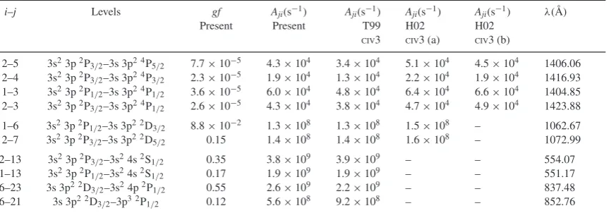
Table 1. A selection of important SIVlines.
i–j Levels gf Aji(s−1) Aji(s−1) Aji(s−1) Aji(s−1) λ(Å)
Present Present T99 H02 H02
CIV3 CIV3 (a) CIV3 (b)
2–5 3s23p2P3
/2–3s 3p2 4P5
/2 7.7×10⁻⁵ 4.3×10⁴ 3.4×10⁴ 5.1×10⁴ 4.5×10⁴ 1406.06 2–4 3s23p2P3
/2–3s 3p2 4P3
/2 2.3×10⁻⁵ 1.9×10⁴ 1.3×10⁴ 2.2×10⁴ 1.9×10⁴ 1416.93 1–3 3s23p2P1/2–3s 3p2 4P1/2 3.6×10⁻⁵ 6.0×10⁴ 4.8×10⁴ 6.4×10⁴ 6.6×10⁴ 1404.85 2–3 3s23p2P3/2–3s 3p2 4P1/2 2.6×10⁻⁵ 4.3×10⁴ 3.8×10⁴ 4.7×10⁴ 4.9×10⁴ 1423.88 1–6 3s23p2P1/2–3s 3p2 2D3/2 8.8×10⁻² 1.3×10⁸ 1.3×10⁸ 1.5×10⁸ – 1062.67 2–7 3s23p2P3/2–3s 3p2 2D5/2 0.15 1.4×10⁸ 1.4×10⁸ 1.6×10⁸ – 1072.99 2–13 3s23p2P3
/2–3s24s2S1
/2 0.35 3.8×10⁹ 3.9×10⁹ – – 554.07
1–13 3s23p2P1
/2–3s24s2S1
/2 0.17 1.9×10⁹ 1.9×10⁹ – – 551.17
6–23 3s 3p2 2D3
/2–3s24p2P1
/2 0.55 2.6×10⁹ 2.2×10⁹ – – 837.48
6–21 3s 3p2 2D3
/2–3p3 2P1
/2 0.12 5.6×10⁸ 9.2×10⁸ – – 852.76
Notes. T99: Tayal (1999)CIV3 calculations. H02: Hibbert et al. (2002)CIV3 calculations. Case (a) refers to the extended orbitals, valence
+core–valence correlations, adjusted. Case (b) refers to the most elaborate calculation, with extended orbitals, valence+core–valence
+core–core correlations, adjusted.
found, confirming that indeed at high densities the problems were still there.CHIANTIv.3 was used. Possible explanations were the
presence of an unidentified blending line (which becomes strong only at high densities), or inaccuracies in the SIVatomic data at
high densities.
It is of particular importance to resolve the 1404.8 Å prob-lem now, since the SIV and O IV lines are routinely observed
since 2013 by theInterface Region Imaging Spectrograph(IRIS; De Pontieu et al.2014) with high temporal, spatial and spectral resolutions.
S IV is an Al-like ion, as FeXIV. Previous scattering
calcula-tions of FeXIVhave clearly shown the limitations of small CI/CC
expansions (see Storey, Mason & Young2000; Liang et al.2010; Del Zanna et al.2015c). The first step is therefore to carry out a larger calculation for SIV. The aim of this paper is to present
a new scattering calculation based on an improved target, and see how the new model ion affects the main diagnostics for this ion.
2 AT O M I C S T R U C T U R E
The atomic structure calculations were carried out using the
AUTOSTRUCTUREprogram (Badnell2011), which originated from the SUPERSTRUCTUREprogramme (Eissner, Jones & Nussbaumer1974),
and which constructs target wavefunctions using radial wavefunc-tions calculated in a scaled Thomas–Fermi–Dirac–Amaldi statisti-cal model potential with a set of sstatisti-caling parameters. The sstatisti-caling parametersλnlfor the potentials in which the orbital functions are calculated are 1s: 1.450 50; 2s: 1.085 76; 2p: 1.032 83; 3s: 1.083 08; 3p: 1.057 53; 3d: 1.090 29; 4s: 1.095 77; 4p: 1.071 59; 4d: 1.111 60; 4f: 1.379 70. For the CI expansion, we have chosen the set of 29 configurations (up ton=4) 3s23p, 3s 3p2, 3s23d, 3s24l (l=s,p,d,f),
3p3, 3s 3p 3d, 3s 3p 4l (l=s,p,d,f), 3s 3d 4l (l=s,p,d,f), 3s 3d2, 3p2
3d, 3p24l (l=s,p,d,f), 3p 3d2, 3p 3d 4l (l=s,p,d,f), 3d3, giving rise
to 298LSterms and 715 fine-structure levels.
An accurate description of spin–orbit mixing between two levels requires their initial term separation to be accurate. This is fre-quently not the case, so the term energy correction (TEC) method, introduced by Zeippen, Seaton & Morton (1977) and Nussbaumer & Storey (1978), was used to improve the term separations.
We first reviewed the wavelength measurements and the ob-served energies as reported by NIST.1We focused on the lowest
levels, which are the most important ones for diagnostic purposes. We found various small inconsistencies, and revised the experi-mental level energiesEexpobtaining excellent consistency. We also
found various incorrect wavelength measurements, especially of the 1404.8 Å line, which are still reported in much of the literature. Details of the revised experimental level energies are given in the appendix.
We then obtained a set of ‘best-guess’ energiesEbestby linear
in-terpolation. We then used theEbestvalues to obtain the TEC values,
then rerunAUTOSTRUCTUREto obtain the corrected target energies
ETEC. The list of the lowest levels is provided in Table A1. We
note that the ordering of some of the levels changes once the TEC are introduced. TheETECenergies are very close to the
experimen-tal values, so were used to calculate the radiative data, still with
AUTOSTRUCTURE. The A-values are very close (within about 10 per cent) to those previously calculated by Hibbert, Brage & Fleming (2002), as shown in Table1. Larger differences with the values calculated by Tayal (1999) are found in some cases.
3 S C AT T E R I N G C A L C U L AT I O N
For the CC expansion, we have retained the lowest 418 levels orig-inating from 175LSterms, to include all the terms of the 3p 3d2
configuration. This represents a significant improvement over the previous calculations by Tayal (2000), where only 24LSterms were included.
TheR-matrix method used in the scattering calculation is de-scribed in Hummer et al. (1993) and Berrington, Eissner & Nor-rington (1995). We performed the calculation in the inner region inLScoupling and included mass and Darwin relativistic energy corrections.
The outer region calculation used the intermediate-coupling frame transformation method (ICFT) described by Griffin, Bad-nell & Pindzola (1998). The ICFT method determines the multi-channel quantum defect theory (MQDT) unphysical (i.e. largely energy independent)LS-coupling reactance matrix and transforms it to intermediate coupling using term coupling coefficients, i.e. it
1http://physics.nist.gov
at University of Strathclyde on October 26, 2016
http://mnras.oxfordjournals.org/
allows for spin–orbit mixing within the target but neglects it for the colliding electron. On using the MQDT expression to transform to the level-resolved physical reactance matrix the closing-off of the unphysical channels gives rise to Rydberg series of resonances converging on the non-degenerate energy levels, as characterized by the tan(πνj) factor. This is discussed in section 2 of Griffin et al. (1998). We used 22 continuum basis functions per orbital to expand the scattered electron partial wavefunction within theR-matrix box. This enabled us to calculate converged collision strengths up to 9 Ryd.
We included exchange up to a total angular momentum quantum number J = 28/2. We have supplemented the exchange contri-butions with a non-exchange calculation extending to J=76/2. The outer region part of the exchange calculation was performed in a number of stages. The resonance region was calculated with an energy resolution of 0.000 78 Ryd (Tayal2000used a resolu-tion of 0.001 Ryd). A coarse energy mesh was chosen above all resonances.
Dipole-allowed transitions were topped-up to infinite partial wave using an intermediate-coupling version of the Coulomb–Bethe method as described by Burgess (1974) while non-dipole allowed transitions were topped-up assuming that the collision strengths form a geometric progression inJ(see Badnell & Griffin2001).
The TECs have been incorporated into the ICFT method as de-scribed in Del Zanna & Badnell (2014). The collision strengths were extended to high energies by interpolation using the appropri-ate high-energy limits in the Burgess & Tully (1992) scaled domain. The high-energy limits were calculated withAUTOSTRUCTUREfor both
optically allowed (see Burgess, Chidichimo & Tully1997) and non-dipole allowed transitions (see Chidichimo, Badnell & Tully2003). The temperature-dependent effective collisions strengthϒ(i− j) were calculated by assuming a Maxwellian electron distribution and linear integration with the final energy of the colliding electron. The full data set is made available at our APAP website2and will be
made available in the future version of theCHIANTI3data base (Dere
et al.1997; Del Zanna et al.2015b).
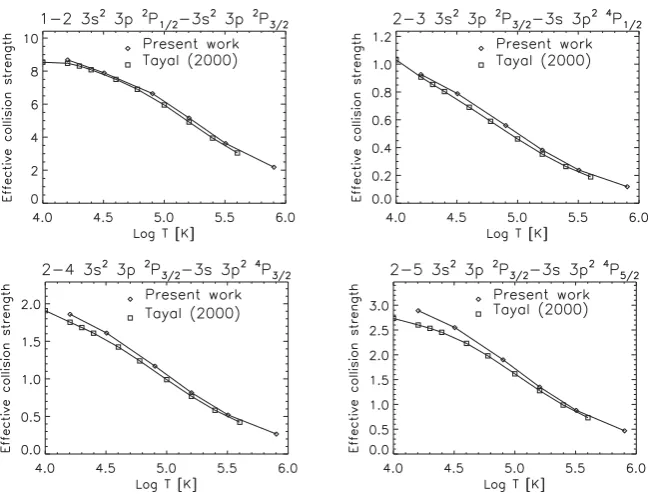
Fig.1shows a comparison with the values calculated by Tayal (2000) at two temperatures, for transitions from the lowest five levels. There is a large scatter, but for most transitions there is agreement within 20 per cent at high temperatures. There is an en-hancement in our collision strengths at lower temperatures, which is normally present when the calculation has a large CC expansion, hence more resonance enhancement. There are, however, several transitions for which large discrepancies are present. We have of-ten found that a larger CI expansion can change considerably the oscillator strengths and collision strengths to the higher levels of a smaller calculation (see e.g. Fern´andez-Menchero, Del Zanna & Badnell2015), so we would expect the large discrepancies to be as-sociated to the last few levels in Tayal (2000) calculation. However, this is not the case, as we show below. We note also that not all tran-sitions that show these discrepancies are relevant for astrophysical applications.
To find out which collision strengths are important for astrophys-ical applications, we have calculated the level populations using the collisions strengths andA-values. They are shown in Fig.2. There are clear discrepancies in the population of the metastable 3s 3p 3d
4F
9/2level. It turns out that this metastable level provides
popula-tion to several higher levels which were not included in the 52-level
[image:3.595.311.541.55.396.2]2www.apap-network.org 3www.chiantidatabase.org
Figure 1. Thermally averaged collision strengths (Tayal2000versus the present ones) for transitions from the lowest five levels only at two different temperatures. Dashed lines indicate±20 per cent.
CHIANTImodel that was based on Tayal (2000) collisions strengths.
Including all the levels and all the excitation and de-excitation pro-cesses lowers significantly the population of the 3s 3p 3d4F
9/2level,
and hence slightly affects the populations of the other important 3s 3p2 4P metastable levels, and of the ground configuration.
The main levels for density diagnostics are the three 3s 3p2 4P
levels, which produce the lines shown in Table1. These levels are populated by excitations from the lower levels, and also by radiative cascading. We have found general agreement between the excita-tions of the main populating transiexcita-tions of the present large-scale calculation and those of Tayal (2000), as shown in Fig.3, although there is a slight increase, especially towards lower temperatures, due to the extra resonance enhancements of the present CC expansion. The combined effects of the larger model and different populations have minor effects on the diagnostic ratios, as shown in Fig.4. The differences are significant at high densities for the 1404.8 Å tran-sition, which is the most important diagnostic line. However, these differences become reduced if the Hibbert et al. (2002) A-values (case a) are used instead.
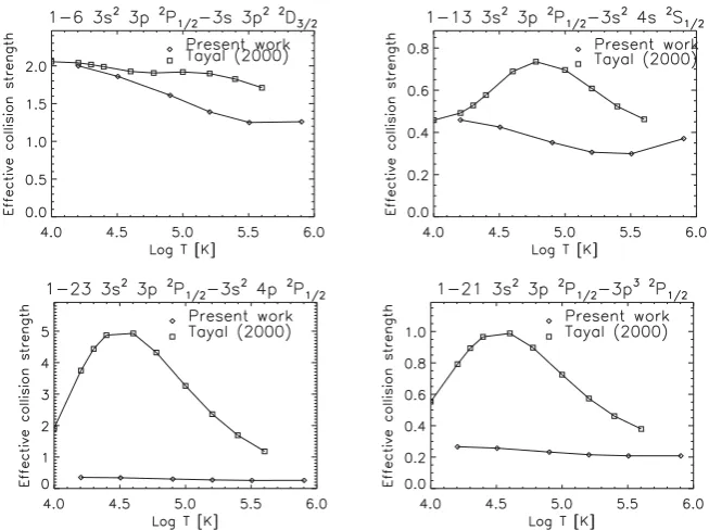
The large discrepancies in Fig.1are often associated with lev-els that do not produce strong transitions. However, a few cases are worth pointing out. The other important diagnostic ratio is the 1062.67/1072.99 Å. The excitation from the ground state to the 3s 3p2 2D
3/2which produces the 1062.67 Å (1–6) line is significantly
different, as shown in Fig.5(top-left plot). OurA-value for the 1–6 line is close to that one calculated by Tayal (2000), as shown in
at University of Strathclyde on October 26, 2016
http://mnras.oxfordjournals.org/
Figure 2. The relative population of the SIVlevels, calculated with Tayal’s data (as in theCHIANTIdata base since v.3) and with the present data.
Figure 4. Two of the main density diagnostic ratios around 1400 Å.
Table1, so the difference is not due to a difference in the atomic structure. Our predicted 1062.67/1072.99 Å ratio, shown in Fig.6, differs from the previousCHIANTImodel.
The decays from the 3s24s2S
1/2level, at 554 and 551 Å (lines
[image:4.595.323.535.60.379.2]1–13 and 2–13 in Table1), are also significantly different, because
Figure 3. Thermally averaged collision strengths for a selection of transitions compared to those calculated by Tayal (2000).
at University of Strathclyde on October 26, 2016
http://mnras.oxfordjournals.org/
[image:4.595.135.460.468.715.2]Figure 5. Thermally averaged collision strengths for a selection of transitions compared to those calculated by Tayal (2000).
Figure 6. The other main density diagnostic ratio in the UV.
of the different collision strength from the ground state, as shown in Fig.5(top-right plot). As in the previous case, ourA-values are close to those of Tayal.
Finally, the decays of several other levels from the 3s24p and
3p3configurations are also significantly different. The most striking
case is the 6–23 3s 3p2 2D
3/2–3s24p2P1/2transition at 837.48 Å.
This transition has been observed in laboratory spectra, but the intensity predicted by our model is almost six times lower than that one calculated with theCHIANTImodel. The reason is the large
discrepancy in the excitation of the forbidden transition from the ground state, as shown in Fig.5(bottom-left plot). Inspection of solar spectra at 837.48 Å clearly indicates that the intensity of this line as predicted by the CHIANTI model is inconsistent with
observations.
A similar large discrepancy occurs for the 6–21 3s 3p2 2D 3/2–
3p3 2P
[image:5.595.45.285.332.521.2]1/2, because of the large difference in the excitation from
Table 2. Level energies.
i Conf. LSJ ET99 ET99 ET00 ET00 Eexp
Ai Adj. Ai Adj.
21 3p3 2P1
/2 212 012 211 310 213 637 210 882 211 375 22 3p3 2P3/2 212 056 211 420 216 215 212 803 211 363 23 3s24p 2P1/2 213 702 213 439 213 264 213 867 213 513 24 3s24p 2P3/2 213 790 213 593 216 259 213 922 213 724
Notes. Energies in kaysers.ET99: energies from the atomic structure
cal-culation of Tayal (1999), ab initio (Ai) and adjusted (Adj.);ET00: energies from the scattering calculation of Tayal (2000);Eexp: present experimental energies.
the ground state, as shown in Fig.5(bottom-right plot). While the above-mentioned differences are not too large, the differences in the excitation to the 3p3 2P
1/2, 3/2and 3s24p2P1/2, 3/2levels are large and
puzzling. The discrepancies cannot be ascribed to more resonance enhancement (given that our CC expansion is much larger), because our collision strengths are actually smaller than those calculated by Tayal. We have also calculated our collision strengths without the TEC corrections, and found similar results. Finally, our collision strengths are consistent with the high-energy limits calculated with
AUTOSTRUCTRUE, so we are confident on the validity of our results.
We have then considered the atomic structure calculation of Tayal (1999), and report in Table2the energies of these four levels, ob-tained with the ab-initio calculation and the one where adjustments to the diagonal elements of the Hamiltonian matrices were applied. We have also compared ourA-values with those reported by Tayal (1999) and did not find large differences. For example, Table 1
shows theA-values for the two main decays from the 3p3 2P 1/2and
4p2P
1/2levels. Tayal (1999) obtained 9.2×10⁸, 2.2×10⁹while
our values are 5.6×10⁸, 2.6×10⁹, respectively. The other decays
have similar differences.
When we looked at the energies in table 1 of Tayal (2000), how-ever, we found two issues. First, the ab initio and adjusted en-ergies of several levels are not the same as those listed in Tayal (1999). This is puzzling, since Tayal (2000) stated to have used the
at University of Strathclyde on October 26, 2016
http://mnras.oxfordjournals.org/
wavefunctions as described in Tayal (1999). If that was the case, we would have expected that the energies in the two papers were the same. Secondly, the two levels which show the large discrepancies (the 3p3 2P
1/2and 4p2P1/2levels) have ab-initio energies in Tayal
(2000) that do not follow the experimental ordering, as also shown in Table2. As described in TableA1, these two levels are highly mixed, so it is possible that Tayal (2000) inverted these two levels. Inverting the ordering of the levels when applying the adjustments to the diagonal elements of the Hamiltonian matrices might be the cause of the large discrepancies.
4 C O M PA R I S O N T O O B S E RVAT I O N S
A full discussion of the SIVand OIVdiagnostics around 1400 Å
is deferred to a future paper. However, we note here that since the present atomic data for SIVare similar to the previous ones for these
lines, previous results based on Tayal’s cross-sections still hold. At low nebular densities, very good agreement between observed and predicted intensities is found. At high densities, the problem in the SIVand OIVblend at 1404.8 Å discussed in Del Zanna et al. (2002) is still present.
As an example, we have considered the solar observations of an active region by the HRTS second rocket flight in 1978 February, described by Brekke et al. (1991). We have fitted the line intensities trying to remove all the blends, in particular the 1423.8 line which is clearly blended when observed at the excellent HRTS spectral resolution.
We show the comparisons in terms of the ‘emissivity ratio’ curves (Del Zanna, Berrington & Mason2004), which are basically the ratios of the observed (Iob, energy units) and the calculated line
emissivities as a function of the electron densityNe:
Rji= N IobNeλji j(Ne, Te)Aji C,
(1)
whereNj(Ne,Te) is the population of the upper leveljrelative to the
total number density of the ion, calculated at a fixed temperature
Te.λji is the wavelength of the transition,Aji is the spontaneous radiative transition probability andCis a scaling constant that is the same for all the lines within one observation. If agreement between experimental and theoretical intensities is present, all lines should be closely spaced or intersect, for a near isodensity plasma. The value ofCis chosen so that the emissivity ratiosRjiare near unity where they intersect.
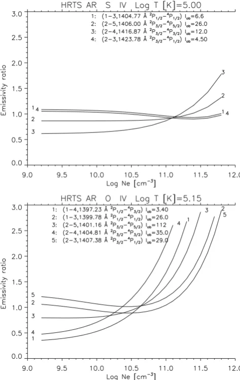
Fig.7(top) shows the emissivity ratio curves obtained from the SIVwith the present atomic data. The intensities of the 1406.0 and
1416.87 Å indicate a density of about 1011.1cm−3, in close
agree-ment with the density obtained from SiIII(Del Zanna,
Fern´andez-Menchero & Badnell2015a). If we adjust the observed intensity of the SIV1404.8 Å, we then obtain an estimate of the intensity of the OIV1404.8 Å line.
Fig.7(bottom) shows the emissivity ratio curves obtained from the OIVlines. For OIVwe have used theCHIANTIv.8 data (Del Zanna
et al.2015b), mainly cross-sections for electron impact excitation from Liang, Badnell & Zhao (2012) andA-values for the lower levels from Corr´eg´e & Hibbert (2004). We note that the proton excitation among the4P levels has some effect on the relative intensities of
the lines within the multiplet.CHIANTIv.8 includes the proton rates
calculated by Foster, Keenan & Reid (1997) using a close-coupled impact-parameter method. The OIVlines indicate a density of about
1010.7 cm−3, slightly lower than the value one would expect for
constant pressure (1010.9cm−3). The estimated intensity of the O IV
[image:6.595.309.546.57.432.2]1404.8 Å line is still about 30 per cent stronger than predicted.
Figure 7. Emissivity ratio curves of the SIVand OIVlines observed during the HRTS second rocket flight on an active region.Iobindicates the observed intensity (erg).
We obtain similar results using stellar UV observations such as those of Capella (Linsky et al.1995; Del Zanna et al.2002). The reasons for the discrepancy could well be the presence of an unknown blend. However, the discrepancy is almost within uncer-tainties, given the marginal density sensitivity of the SIVaround
1011cm−3. Another possibility is that proton excitation also affects
the SIV4P levels. In the literature, we have only found some
esti-mates by Bhatia, Doschek & Feldman (1980) for the rates for proton excitation among two of the4P levels. They were obtained using
a semi-classical technique (Kastner & Bhatia1979) and are quite uncertain. Adding these estimates does not affect significantly the populations of the4P levels; however, more accurate calculations
would be needed before reaching any definitive conclusions.
5 C O N C L U S I O N S
Despite having run a calculation with much larger CI/CC expansions than Tayal (2000), we have obtained similar populations for the three 3s 3p2 4P levels, important for density diagnostics. We confirm
that there is still a discrepancy with the important 1404.8 Å line, blend of OIVand SIV. Large problems with the atomic data are
now ruled out, so blending with an unknown line is still a possible
at University of Strathclyde on October 26, 2016
http://mnras.oxfordjournals.org/
explanation. We are currently reviewingIRISobservations of several solar flares and active regions to assess if the discrepancy is a common feature.
We found significant differences in the 1062.7 and 1073.0 Å lines, useful for diagnostics in low-density plasma such as in nebulae. We also found an inconsistency in the level population for this ion as calculated within theCHIANTIdata base and related to the 3s 3p 3d 4F
9/2metastable level.
Several inconsistencies in the collision strengths of other tran-sitions calculated by Tayal (2000) have been found, as shown in Figs1and5. We are confident that our atomic data can reliably be used for astrophysical applications.
AC K N OW L E D G E M E N T S
This work was funded by STFC (UK) through the University of Cambridge DAMTP astrophysics grant and the University of Strathclyde UK APAP network grant ST/J000892/1. We would like to thank the anonymous referee for useful comments on the manuscript.
R E F E R E N C E S
Badnell N. R., 2011, Comput. Phys. Commun., 182, 1528
Badnell N. R., Griffin D. C., 2001, J. Phys. B: At. Mol. Phys., 34, 681 Berrington K. A., Eissner W. B., Norrington P. H., 1995, Comput. Phys.
Commun., 92, 290
Bhatia A. K., Doschek G. A., Feldman U., 1980, A&A, 86, 32 Bowen I. S., 1928, Phys. Rev., 31, 34
Brage T., Judge P. G., Brekke P., 1996, ApJ, 464, 1030
Brekke P., Kjeldseth-Moe O., Bartoe J.-D. F., Brueckner G. E., 1991, ApJS, 75, 1337
Burgess A., 1974, J. Phys. B: At. Mol. Phys., 7, L364 Burgess A., Tully J. A., 1992, A&A, 254, 436
Burgess A., Chidichimo M. C., Tully J. A., 1997, J. Phys. B: At. Mol. Phys., 30, 33
Burton W. M., Ridgeley A., 1970, Sol. Phys., 14, 3
Chidichimo M. C., Badnell N. R., Tully J. A., 2003, A&A, 401, 1177 Cook J. W., Keenan F. P., Dufton P. L., Kingston A. E., Pradhan A. K.,
Zhang H. L., Doyle J. G., Hayes M. A., 1995, ApJ, 444, 936 Corr´eg´e G., Hibbert A., 2004, At. Data Nucl. Data Tables, 86, 19 De Pontieu B. et al., 2014, Sol. Phys., 289, 2733
Del Zanna G., Badnell N. R., 2014, A&A, 570, A56
Del Zanna G., Landini M., Mason H. E., 2002, A&A, 385, 968 Del Zanna G., Berrington K. A., Mason H. E., 2004, A&A, 422, 731 Del Zanna G., Fern´andez-Menchero L., Badnell N. R., 2015a, A&A, 574,
A99
Del Zanna G., Dere K. P., Young P. R., Landi E., Mason H. E., 2015b, A&A, 582, A56
Del Zanna G., Liang G. Y., Badnell N. R., Fern´andez-Menchero L., Liang G. Y., Mason H. E., Storey P. J., 2015c, MNRAS, 454, 2909
Dere K. P., Landi E., Mason H. E., Monsignori Fossi B. C., Young P. R., 1997, A&AS, 125, 149
Dere K. P., Landi E., Young P. R., Del Zanna G., 2001, ApJS, 134, 331 Dufton P. L., Hibbert A., Kingston A. E., Doschek G. A., 1982, ApJ, 257,
338
Eissner W., Jones M., Nussbaumer H., 1974, Comput. Phys. Commun., 8, 270
Ekberg J. O., Åke Svensson L., 1970, Phys. Scr., 2, 283 Feldman U., Doschek G. A., 1979, A&A, 79, 357 Feldman U., Doschek G. A., 1991, ApJS, 75, 925
Fern´andez-Menchero L., Del Zanna G., Badnell N. R., 2015, MNRAS, 450, 4174
Feuchtgruber H. et al., 1997, ApJ, 487, 962 Flower D. R., Nussbaumer H., 1975, A&A, 45, 145
Foster V. J., Keenan F. P., Reid R. H. G., 1997, At. Data Nucl. Data Tables, 67, 99
Griffin D. C., Badnell N. R., Pindzola M. S., 1998, J. Phys. B: At. Mol. Phys., 31, 3713
Harper G. M., Jordan C., Judge P. G., Robinson R. D., Carpenter K. G., Brage T., 1999, MNRAS, 303, L41
Hibbert A., Brage T., Fleming J., 2002, MNRAS, 333, 885
Hummer D. G., Berrington K. A., Eissner W., Pradhan A. K., Saraph H. E., Tully J. A., 1993, A&A, 279, 298
Kastner S. O., Bhatia A. K., 1979, A&A, 71, 211
Kaufman V., Martin W. C., 1993, J. Phys. Chem. Ref. Data, 22, 279 Keenan F. P. et al., 2002, MNRAS, 337, 901
Liang G. Y., Badnell N. R., Crespo L´opez-Urrutia J. R., Baumann T. M., Del Zanna G., Storey P. J., Tawara H., Ullrich J., 2010, ApJS, 190, 322 Liang G. Y., Badnell N. R., Zhao G., 2012, A&A, 547, A87
Linsky J. L., Wood B. E., Judge P., Brown A., Andrulis C., Ayres T. R., 1995, ApJ, 442, 381
Millikan R. A., Bowen I. S., 1925, Phys. Rev., 25, 600 Nussbaumer H., Storey P. J., 1978, A&A, 64, 139
Rank D. M., Holtz J. Z., Geballe T. R., Townes C. H., 1970, ApJ, 161, L185 Sandlin G. D., Bartoe J.-D. F., Brueckner G. E., Tousey R., Vanhoosier
M. E., 1986, ApJS, 61, 801
Storey P. J., Mason H. E., Young P. R., 2000, A&AS, 141, 285 Tayal S. S., 1999, J. Phys. B: At. Mol. Phys., 32, 5311 Tayal S. S., 2000, ApJ, 530, 1091
Young P. R., Feldman U., Lobel A., 2011, ApJS, 196, 23
Zeippen C. J., Seaton M. J., Morton D. C., 1977, MNRAS, 181, 527
A P P E N D I X A : E N E R G I E S
TableA1provides a comparison of target level energies. We have slightly revised the energies of several levels and provide new exper-imental energiesEexp. The changes, compared to the NIST values
(ENIST) might appear negligible (a few kaysers at most), but are
needed to provide accurate wavelength measurements. These are nowadays required, given the high-resolution of current spectrom-eters such as theIRISmission, to obtain accurate measurements of Doppler shifts.
Only the lowest levels, corresponding to the 52 levels of Tayal’s calculation are shown here. We include 69 levels because Tayal did not include the 3s 3p 4p levels. TableA1also shows the target energiesEtand those obtained with the TEC,ETEC.
Most of the literature values that we adopt for the EUV lines are from Millikan & Bowen (1925) and Bowen (1928). The mea-surements appear accurate to within a few mÅ. Kaufman & Martin (1993) provided a list of unpublished measurements which had an uncertainty of about 0.02 Å below 2000 Å and 0.03 Å above 2000 Å. The Kaufman & Martin (1993) are generally consistent with those measured by Bowen.
In terms of solar data, the most accurate wavelength measure-ments in the UV were obtained from severalSkylabspectra at the limb, as reported by Sandlin et al. (1986). Their accuracy is about 0.005 Å, so we prefer these data over the laboratory measurements. In principle, accurate measurements for the UV lines could also be obtained fromHST/STIS spectra of nebulae. However, line pro-files are often not symmetric, and discrepancies in the measurements are present. We note that the RR Tel measurements of Young, Feld-man & Lobel (2011) are relatively close to the solar ones, but those of Keenan et al. (2002) are incorrect, as already noted by Young et al. (2011), probably because of a problem in the wavelength calibration.
In what follows we provide some details of our revised energies for the lowest levels.
at University of Strathclyde on October 26, 2016
http://mnras.oxfordjournals.org/
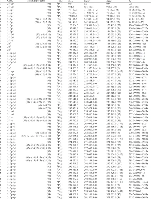
Table A1. Level energies.
i Conf. Mixing (per cent) LSJ Eexp ENIST ETEC Et
1 3s23p (94) 2P1
/2 0.0 0.0 0.0 0.0
2 3s23p (94) 2P3
/2 951.4 951.4 (0) 918.0 (33) 918.0 (33)
3 3s 3p2 (98) 4P1
/2 71 182.0 71 184.1 (−2) 71 182.0 (0) 68 963.0 (2219)
4 3s 3p2 (98) 4P3
/2 71 526.6 71 528.7 (−2) 71 512.0 (15) 69 292.0 (2235)
5 3s 3p2 (98) 4P5
/2 72 072.2 72 074.4 (−2) 72 042.0 (30) 69 823.0 (2249) 6 3s 3p2 (79)+11(c3 17) 2D3/2 94 102.5 94 103.1 (−1) 94 083.0 (20) 94 141.0 (−39) 7 3s 3p2 (79)+12(c3 17) 2D5/2 94 148.0 94 150.3 (−2) 94 126.0 (22) 94 183.0 (−35)
8 3s 3p2 (96) 2S1/2 123 504.5 123 509.3 (−5) 123 483.0 (22) 126 476.0 (−2972)
9 3s 3p2 (93) 2P1/2 133 619.0 133 619.6 (−1) 133 612.0 (7) 136 841.0 (−3222)
10 3s 3p2 (93) 2P3/2 134 243.2 134 245.4 (−2) 134 214.0 (29) 137 443.0 (−3200)
11 3s23d (77)+6(c2 16) 2D3
/2 152 128.3 152 133.2 (−5) 152 093.0 (35) 156 489.0 (−4361)
12 3s23d (77)+7(c2 16) 2D5
/2 152 141.3 152 146.8 (−6) 152 127.0 (14) 156 523.0 (−4382)
13 3s24s (94) 2S1
/2 181 432.0 181 448.2 (−16) 181 410.0 (22) 182 750.0 (−1318)
14 3p3 (56)+33(c6 41) 2D3
/2 185 055.2 185 055.2 (0) 185 030.0 (25) 183 893.0 (1162)
15 3p3 (56)+32(c6 41) 2D5
/2 185 146.7 185 148.0 (−1) 185 128.0 (19) 183 989.0 (1158)
16 3p3 (97) 4S3
/2 196 453.7 196 455.4 (−2) 196 431.0 (23) 196 320.0 (134)
17 3s 3p 3d (98) 4F3
/2 203 442.8 203 442.8 (0) 203 427.0 (16) 203 112.0 (331)
18 3s 3p 3d (98) 4F5
/2 203 632.8 203 632.8 (0) 203 617.0 (16) 203 302.0 (331)
19 3s 3p 3d (98) 4F7
/2 203 906.3 203 906.3 (0) 203 886.0 (20) 203 571.0 (335)
20 3s 3p 3d (98) 4F9
/2 204 264.9 204 264.9 (0) 204 236.0 (29) 203 921.0 (344) 21 3p3 (40)+44(c6 15)+23(c7 34) 2P1
/2 211 374.8 211 366.6 (8) 211 330.0 (45) 212 904.0 (−1529) 22 3p3 (44)+43(c6 16)+24(c7 28) 2P3
/2 211 363.0 211 376.3 (−13) 211 357.0 (6) 212 929.0 (−1566)
23 3s24p (58)+21(c5 27) 2P1
/2 213 513.0 213 514.7 (−2) 213 525.0 (−12) 215 598.0 (−2085) 24 3s24p (64)+22(c5 23) 2P3/2 213 724.0 213 725.3 (−1) 213 677.0 (47) 215 750.0 (−2026)
25 3s 3p 3d (96) 4P5/2 222 198.0 222 198.3 (0) 222 191.0 (7) 222 375.0 (−177)
26 3s 3p 3d (96) 4P3/2 222 487.5 222 488.6 (−1) 222 447.0 (41) 222 631.0 (−144)
27 3s 3p 3d (97) 4P1/2 222 692.0 222 692.4 (0) 222 624.0 (68) 222 802.0 (−110)
28 3s 3p 3d (97) 4D1
/2 224 339.4 224 342.7 (−3) 224 315.0 (24) 225 004.0 (−665)
29 3s 3p 3d (96) 4D3
/2 224 443.0 224 435.6 (7) 224 406.0 (37) 225 090.0 (−647)
30 3s 3p 3d (96) 4D5
/2 224 537.0 224 539.3 (−2) 224 516.0 (21) 225 199.0 (−662)
31 3s 3p 3d (98) 4D7
/2 224 617.8 224 617.3 (1) 224 612.0 (6) 225 304.0 (−686) 32 3s 3p 3d (39)+15(c5 23)+52(32) 2D5
/2 233 610.4 233 610.4 (0) 233 593.0 (17) 236 149.0 (−2539) 33 3s 3p 3d (39)+14(c5 23)+51(32) 2D3
/2 233 641.7 233 641.7 (0) 233 616.0 (26) 236 173.0 (−2531)
34 3s 3p 3d (68)+48(28) 2F5
/2 241 646.3 241 646.3 (0) 241 645.0 (1) 246 245.0 (−4599)
35 3s 3p 3d (68)+47(28) 2F7
/2 242 421.4 242 421.4 (0) 242 385.0 (36) 246 985.0 (−4564)
36 3s24d (94) 2D3
/2 255 395.8 255 395.8 (0) 255 368.0 (28) 257 421.0 (−2025)
37 3s24d (94) 2D5
/2 255 400.3 255 400.3 (0) 255 383.0 (17) 257 436.0 (−2036) 38 3s24f (57)+35(c6 15)+47(c6 24) 2F7
/2 257 611.0 257 611.0 (0) 257 611.0 (0) 261 963.0 (−4352) 39 3s24f (57)+34(c6 15)+48(c6 24) 2F5
/2 257 742.6 257 742.6 (0) 257 692.0 (51) 262 045.0 (−4302)
40 3s 3p 4s (98) 4P1
/2 263 097.1 263 097.1 (0) 263 171.0 (−74) 263 609.0 (−512)
41 3s 3p 4s (98) 4P3
/2 263 448.1 263 448.1 (0) 263 466.0 (−18) 263 907.0 (−459)
42 3s 3p 4s (98) 4P5/2 264 067.7 264 067.7 (0) 263 984.0 (84) 264 420.0 (−352)
43 3s 3p 3d (68)+22(c5 15) 2P3/2 264 882.8 264 882.8 (0) 264 880.0 (3) 270 921.0 (−6038) 44 3s 3p 3d (67)+21(c5 14)+45(c10 12) 2P1/2 265 055.1 265 055.1 (0) 265 002.0 (53) 271 045.0 (−5990) 45 3s 3p 4s (83) 2P1/2 270 826.7 270 826.7 (0) 270 897.0 (−70) 275 915.0 (−5088)
46 3s 3p 4s (85) 2P3
/2 271 436.9 271 436.9 (0) 271 372.0 (65) 276 388.0 (−4951) 47 3s 3p 3d (42)+35(13)+38(c9 38) 2F7
/2 277 596.0 277 596.0 (0) 277 561.0 (35) 285 256.0 (−7660) 48 3s 3p 3d (42)+34(13)+39(c9 37) 2F5
/2 277 682.9 277 682.9 (0) 277 680.0 (3) 285 374.0 (−7691)
49 3s 3p 3d (83) 2P1
/2 278 676.9 278 676.9 (0) 278 611.0 (66) 286 990.0 (−8313)
50 3s 3p 3d (83) 2P3
/2 278 642.4 278 642.4 (0) 278 654.0 (−12) 287 024.0 (−8382) 51 3s 3p 3d (60)+14(c5 15)+33(15) 2D3
/2 281 093.6 281 093.6 (0) 281 066.0 (28) 288 385.0 (−7291) 52 3s 3p 3d (60)+15(c5 15)+32(16) 2D5
/2 281 231.6 281 231.6 (0) 281 209.0 (23) 288 520.0 (−7288)
53 3s 3p 4p (86) 2P1
/2 292 569.2 292 569.2 (0) 292 372.0 (197) 293 627.0 (−1058)
54 3s 3p 4p (90) 2P3
/2 292 893.9 292 893.9 (0) 292 620.0 (274) 293 749.0 (−855)
55 3s 3p 4p (89) 4D1
/2 293 310.8 293 310.8 (0) 293 372.0 (−61) 293 042.0 (269)
56 3s 3p 4p (93) 4D3
/2 293 463.1 293 463.1 (0) 293 526.0 (−63) 293 322.0 (141)
57 3s 3p 4p (98) 4D5
/2 293 736.6 293 736.6 (0) 293 811.0 (−74) 293 793.0 (−56)
58 3s 3p 4p (98) 4D7
/2 294 282.2 294 282.2 (0) 294 288.0 (−6) 294 266.0 (16)
59 3s 3p 4p (97) 4P1
/2 297 397.1 297 397.1 (0) 297 427.0 (−30) 300 863.0 (−3466)
60 3s 3p 4p (96) 4P3/2 297 592.7 297 592.7 (0) 297 591.0 (2) 301 085.0 (−3492)
61 3s 3p 4p (97) 4P5/2 298 010.3 298 010.3 (0) 297 922.0 (88) 301 355.0 (−3345)
62 3s 3p 4p (97) 4S3/2 299 369.3 299 369.3 (0) 299 406.0 (−37) 299 278.0 (91)
63 3s 3p 4p (94) 2D3/2 301 109.8 301 109.8 (0) 301 065.0 (45) 304 748.0 (−3638)
64 3s 3p 4p (94) 2D5
/2 301 576.4 301 576.4 (0) 301 572.0 (4) 305 256.0 (−3680)
at University of Strathclyde on October 26, 2016
http://mnras.oxfordjournals.org/
Table A1 –continued.
i Conf. Mixing (per cent) LSJ Eexp ENIST ETEC Et
65 3p23d (57)+136(21)+186(c15 16) 2F5
/2 – – 307 653.0 310 103.0
66 3p23d (58)+137(21)+187(c15 16) 2F7
/2 – – 308 001.0 310 451.0
67 3s 3p 4p (94) 2S1
/2 308 761.0 308 761.0 (0) 308 741.0 (20) 314 201.0 (−5440)
68 3s 3p 4s (93) 2P1
/2 308 939.3 308 939.3 (0) 308 913.0 (26) 313 410.0 (−4471)
69 3s 3p 4s (93) 2P3
/2 308 996.2 308 996.2 (0) 308 977.0 (19) 313 473.0 (−4477)
Notes. Energies in Kaysers. Only the lowest levels, corresponding to the 52 levels of Tayal’s calculation are shown here (Tayal did not include the 3s 3p 4p
levels).Eexp: present experimental energies;ENIST: NIST experimental energies;ETECpresent calculation with TEC;Et: our ab-initio theoretical energies (without TECs). Values in brackets show differences with our experimental values.
The separation of the 3s2 3p2P
3/2, 1/2 levels is obtained from
measurements of the forbidden line in planetary nebulae; see e.g. Rank et al. (1970) and Feuchtgruber et al. (1997). We adopt the value of 951.4 kayser.
The 1–3 transition is blended with a much stronger OIVline,
so the energy of level no. 3 (3s 3p2 4P
1/2) is obtained from the
2–3 transition, for which we choose the 1423.885±0.005 Å wave-length, measured by Sandlin et al. (1986). We note that our HRTS measurement is 1423.84 Å, the same as the Kaufman & Martin (1993) value, while Young et al. (2011) report 1423.86±0.03 Å. Keenan et al. (2002) report instead a much lower value, 1423.79 Å. Our choice implies that the 1–3 transition should fall at 1404.85 Å. Ekberg & Åke Svensson (1970) identified this line, but reported a solar wavelength of 1404.77 Å, noting that this line is masked with the much stronger OIVline. The solar wavelength of the OIVline
at 1404.77 Å was obtained from Burton & Ridgeley (1970), but the measurement was not very accurate. This wavelength was unfortu-nately later reported in following compilations, including Sandlin et al. (1986). We note that the wavelength of the OIVline as given
by Sandlin et al. (1986) is 1404.82±0.01 Å, so it appears that the OIVand SIVlines are very close.
Level no. 4 (3s 3p2 4P
3/2) produces a weak decay to the ground
state, and a stronger 2–4 transition. We choose the Sandlin et al. (1986) measurement, 1416.928±0.005 Å, which implies that the decay to ground state should be at 1398.08 Å. We note that this decay was observed by Keenan et al. (2002) in the RR Tel spectrum, and that their STIS measurements (1398.044, 1416.872 Å) are relatively close, once a shift of 0.04 Å is applied.
The energy of level no. 5 (3s 3p2 4P
5/2) is obtained from the 2–5
transition, observed at 1406.059±0.005 Å by Sandlin et al. (1986). The energy of level no. 6 is obtained from the 1–6 and 2–6 transi-tions, observed at 1062.672 and 1073.522 Å by Bowen (1928). The energy of level no. 7 is obtained from the 2–7 transition, observed at 1072.992 Å by Bowen (1928).
The energy of level no. 8 is obtained from the 1–8 and 2–8 transitions, observed by Millikan & Bowen (1925) at 809.69 and 815.97 Å, respectively. The energy of level no. 9 is obtained from
the 1–9 and 2–9 transitions, observed by Millikan & Bowen (1925) at 748.40 and 753.76 Å, respectively. The energy of level no. 10 is obtained from the 1–10 and 2–10 transitions, observed by Millikan & Bowen (1925) at 744.92 and 750.23 Å, respectively.
The energy of level no. 11 is obtained from the 1–11 657.34 Å line observed by Millikan & Bowen (1925). The energy of level no. 12 is obtained from the 2–12 661.42 Å line observed by Millikan & Bowen (1925). The energy of level no. 13 is obtained from the 1–13 551.17 Å line observed by Millikan & Bowen (1925).
The level no. 16 is quite important because there are three transi-tions, 3–16, 4–16 and 5–16, observed by Bowen (1928) at 798.265, 800.470 and 803.975 Å, that allow a consistency check of the rel-ative energies of the three4P
1/2levels. We have indeed agreement
within 1 kayser for the energy of level no. 16, assuming the Bowen (1928) measurements and our adopted energies for the4P
1/2levels.
We note that such excellent agreement is not obtained with other choices of wavelength measurements.
The energy of level no. 21 is obtained from the 6–21 transition, observed at 852.716 Å by Bowen (1928).
Level 22 produces several weak lines. The strongest is the 7–22, observed by Bowen (1928) at 853.135 Å. We note a discrepancy in the energy obtained from the 9–22 transition, which should not be the line observed at 1286.063 Å, but the line observed at 1286.22 Å. The energies obtained from the 8–22 (1138.227 Å) and 10–22 (1296.64 Å) are in agreement within 3 kayser.
The energy of level no. 23 is obtained from the 6–23 transition, observed at 837.447 Å by Bowen (1928). The energy of level no. 24 is obtained from the 7–24 transition, observed at 836.286 Å by Bowen (1928).
Finally, the energies of the other levels are either slightly modified adopting the measurements reported by Kaufman & Martin (1993), or are left unaltered as they are in the NIST data base.
This paper has been typeset from a TEX/LATEX file prepared by the author.
at University of Strathclyde on October 26, 2016
http://mnras.oxfordjournals.org/