Evolutionary graph theory revisited: when is an evolutionary process equivalent to the Moran process?

(1)

City, University of London Institutional Repository

Citation

:

Pattni, K., Broom, M., Rychtar, J. & Silvers, L. J. (2015). Evolutionary graph

theory revisited: when is an evolutionary process equivalent to the Moran process?.

Proceedings of the Royal Society A: Mathematical, Physical and Engineering Sciences, 471,

e2182. doi: 10.1098/rspa.2015.0334

This is the accepted version of the paper.

This version of the publication may differ from the final published

version.

Permanent repository link:

http://openaccess.city.ac.uk/13209/

Link to published version

:

http://dx.doi.org/10.1098/rspa.2015.0334

Copyright and reuse:

City Research Online aims to make research

outputs of City, University of London available to a wider audience.

Copyright and Moral Rights remain with the author(s) and/or copyright

holders. URLs from City Research Online may be freely distributed and

linked to.

(2)

rspa.royalsocietypublishing.org

Research

Article submitted to journal

Subject Areas: 92D25, 60J80, 60J20

Keywords:

finite population, evolutionary dynamics, Moran process, fixation probability

Author for correspondence: Karan Pattni

e-mail: [email protected]

Mark Broom

Jan Rychtáˇr

Lara J. Silvers

Evolutionary graph theory

revisited: when is an

evolutionary process

equivalent to the Moran

process?

Karan Pattni

1

, Mark Broom

1

, Jan Rychtáˇr

2

and Lara J. Silvers

1

1_{Department of Mathematics, City University London,}

Northampton Square, London, EC1V 0HB, UK 2_{Department of Mathematics and Statistics, The}

University of North Carolina at Greensboro,

Greensboro, NC 27412, USA

Evolution in finite populations is often modelled using the classical Moran process. Over the last ten years this methodology has been extended to structured populations using evolutionary graph theory. An important question in any such population, is whether a rare mutant has a higher or lower chance of fixating (the fixation probability) than the Moran probability, i.e. that from the original Moran model, which represents an unstructured population. As evolutionary graph theory has developed, different ways of considering the interactions between individuals through a graph and an associated matrix of weights have been considered, as have a number of important dynamics. In this paper we revisit the original paper on evolutionary graph theory in light of these extensions to consider these developments in an integrated way. In particular we find general criteria for when an evolutionary graph with general weights satisfies the Moran probability for the set of six common evolutionary dynamics.

1

c

(3)

2

rspa.ro

y

alsocietypub

lishing.org

Proc

R

Soc

A

0000000

..

1. Introduction

2

When modelling population evolution we are concerned with the spread of heritable 3

characteristics in successive generations. The type of model that is used depends upon whether 4

the population size is assumed to be finite or infinite. The majority of classical evolutionary 5

models (see for example [1,2]) use infinite populations, although finite population models are 6

also well established, the most important models being those in [3,4]. These models are stochastic, 7

and are solved using classical Markov chain methodology [5,6,7]. See also [8,9] for an extension 8

to evolutionary games in finite populations. 9

The populations in the models described above, however, were “well-mixed”, i.e. every 10

individual was equally likely to encounter every other individual. Real populations of course 11

contain structural elements, such as geographical location or social relationship, which mean that 12

some pairs individuals are more likely to interact than others. In such circumstances we need to 13

be able to identify distinct individuals (or at least distinct classes of individuals), and considering 14

finite populations is perhaps more natural than infinite ones (although finite structures each 15

containing an infinite number of individuals, so called “island models”, were considered in [10]). 16

In [11] the modelling ideas of [3] were extended to consider such structured populations based 17

upon graphs, known as evolutionary graph theory. This has proved very successful, spawning a 18

large number of papers (for example [12,13,14,15,16,17,18,19]). For informative reviews see 19

[20,21]. 20

In an evolving population, we need to consider the mechanism of how the population changes, 21

called the dynamics. Informally, the dynamics specify the way in which heritable characteristics 22

are passed on from one generation to the next. For infinite populations the classical replicator 23

equation [22] is often used (although there are a number of alternatives), and in the stochastic 24

model of [3] there is a natural replacement dynamics built in. For structured populations this issue 25

is actually considerably more complex, and the order of births and deaths, and where selection 26

acts, is of vital importance [23,24]. We shall consider a set of dynamics that are commonly used 27

in evolutionary graph theory models. The relationship between dynamics and structure is of 28

key interest because the spread of heritable characteristics is directly dependent upon it. Whilst 29

having essentially no effect on populations with no structure, for constant fitness this relationship 30

potentially yields very different results on graphs. For non-constant fitness the results will vary 31

for different dynamics even in well-mixed populations [25]. 32

Under some circumstances it is, however, possible for the dynamics and structure to interact 33

in such a way that the spread of heritable characteristics behaves just as if the population was 34

homogeneous. This was a central theme of the classic paper [11], where two important results, 35

the circulation theorem and the isothermal theorem, were developed that addressed this question 36

(see also [26] for related work). In this paper we generalise the work of [11] to obtain a complete 37

classification of when the combination of a population structure and dynamics can be regarded 38

as equivalent to a homogeneous population in a precisely defined way, for the six most common 39

evolutionary dynamics and graphs with general weights. 40

2. The Model

41

We shall first describe the population model of [11], which generalises the model of [3] by 42

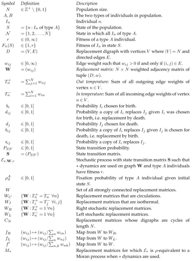
incorporating a replacement structure. The notation used in this paper is summarised in Table1. 43

The population has a constant sizeN∈Z,N≥2, consisting of individualsI1, . . . , IN. Every individual

44

is either of typeAorB.

45

This implies that there are2N different states of the population given by the combination of 46

typeAandBindividuals. We represent each state by a setSsuch thatn∈Sif an individualIn

47

is of typeA. We can easily revert to using the number of typeAindividuals,|S|, if the population 48

is homogeneous. The states ∅ and N=_{1,2, . . . , N_} have only type B and A individuals 49

(4)

3

rspa.ro

y

alsocietypub

lishing.org

Proc

R

Soc

A

0000000

..

Individuals have a constant fitness that may depend upon their type.

51

The fitness of individuals in state S is thus given by the vector F(S) = (Fn(S))n=1,2,...,N

52

where 53

Fn(S) =

(

1 n /∈S,

r_∈(0,_∞) n_∈S,

54 55

is the fitness ofIn. Here the fitnessrof a typeAindividual is given relative to the fitness of a type

56

Bindividual assumed to be 1. 57

During a stochastic replacement event (that happens in an instant) an exact copy of an individualIi

58

replaces an individualIj.

59

The replacement events may be restricted in the sense that not all individuals can replace 60

one another. To enforce such restrictions, [11] imposed a replacement structure using a weighted 61

directed graph given by the tuple (D, w)whereD= (V, E)is a directed graph, with setsV of 62

vertices andE of directed edges, andwis a map that assigns a weight to each edge such that 63

w:V _×V _→[0,_∞) : (i, j)_7→wij. Each vertexn∈V representsInthereforeV ={1,2, . . . , N}so

64

|V_|=N. We assume that(i, j)_∈Eif and only ifwij>0, which indicates thatIican replaceIj.

65

Note that we allowwii>0and thereforeIican replace itself. All the information contained within

66

the weighted digraph (D, w) is conveniently summarised by the N×N weighted adjacency 67

matrixW= (wij)and therefore we will refer to(D, w)usingW, which we call thereplacement

68

matrix. 69

The replacement events are stochastic which means that there is a probability rij=

70

rij(F(S),W)associated with (a copy of)IireplacingIj. There are several potentialevolutionary

71

dynamics on graphs that govern how the probability is determined. There three main types of 72

dynamics that are summarised below, see also [21]. We use the convention thatIiis chosen for

73

birth andIjis chosen for death.

74

(i)Birth-Death(BD):Iiis chosen first thenIj. We have thati∈V is chosen with probability

75

biand then(i, j)∈Ei is chosen with probabilitydij, whereEiare all edges starting in

76

vertexi.dijis used to signify that there is ‘replacement by death’. Finally,rij=bidij.

77

(ii)Death-Birth(DB):Ijis chosen first thenIi. We have thatj∈V is chosen with probability

78

dj and then(i, j)∈Ejis chosen with probabilitybij, whereEjare all edges ending in

79

vertexj.bijis used to signify that there is ‘replacement by birth’. Finally,rij=dibij.

80

(iii)Link(L):IiandIjare chosen simultaneously. In this case(i, j)∈Eis simply chosen with

81

probabilityrij.

82

For each type of these dynamics, the natural selection can, through the fitness parameter, influence 83

either the choice at birth (resulting in adding “B”) or at death (adding “D”). It yields 6 kinds of 84

evolutionary dynamics on graphs summarized in Table2. These dynamics have been extensively 85

studied, in particular, see [27] for a detailed comparison of them. Of these, the BDB and LB 86

dynamics were used in [11]. 87

(a) The fixation probability

88

The fixation probability,ρAS =ρAS(∗,W, r), is the probability that the population with initial state

89

Sis absorbed inN where∗is the dynamics being used. 90

Given that the replacement events are random, the transitions between the states of the 91

population are described by a stochastic process, which we denote E. The properties of E

92

(5)

4

rspa.ro

y

alsocietypub

lishing.org

Proc

R

Soc

A

0000000

..

PSS0=P_SS0(∗,W, r), are calculated using the replacement probabilities as follows: 94

PSS0=                   

X

i /∈S

rij(F(S),W) ifS0=S\ {j}for somej∈S,

X

i∈S

rij(F(S),W) ifS0=S∪ {j}for somej /∈S,

X

i,j∈S

∨i,j /∈S

rij(F(S),W) ifS0=S.

95

96

The transition probabilities,PSS0, satisfy the Markov property because they only depend upon 97

the state S, that is, the probability of transitioning from the present state to another state is 98

independent of any past and future state of the population. The stochastic processE∗,W,rwith

99

state transition matrixS=S(_∗,W, r) = (PSS0)_S,S0_⊂{₁_,₂_,...,N_} is therefore a Markov chain. The 100

Markov chainE∗,W,ris part of the class of evolutionary Markov chains described in [28].

101

The absorbing states ofE∗,W,rare∅,N, which means that if the population is in either one of

102

these states then it remains there indefinitely. This property ofE∗,W,rcan be used to measure the

103

success of a typeAindividual by calculating the probability that it fixates, that is, everyone in the 104

population is of typeA. The fixation probability is then given by solving 105

ρAS=

X

S0_⊂{₁_,₂_,...,N_}

PSS0ρA_S0 (2.1)

106 107

with boundary conditionsρA_∅ = 0andρA_N= 1. 108

As demonstrated in [27], LB and LD dynamics may differ in time scale but they yield the 109

same fixation probabilities when fitness is constant (which is our case). Thus, for our purposes 110

the dynamics are the same and we will thus consider them together and denote them by L. 111

Fixation probability is not the only measure for evolutionary success and we can look at the 112

fixation time [29,30] as well. 113

(b) The Moran Process

114

The Moran process [3], a stochastic birth-death process on finite fixed homogenous population, 115

can be reconstructed asEBDB,WH,rfor a constant replacement matrix 116

WH= (1/N)i,j. (2.2)

117 118

For any r∈(0,∞)and any S⊂ {1, . . . , N}, the fixation probability for this process, orMoran

119

probability, is given by 120

ρAS =

    

1₋r−|S|

1−r−N ifr6= 1,

|S_|/N ifr= 1.

121

122

We are interested in characterizing graphs (and evolutionary dynamics) that yield the same 123

fixation probabilities as the homogeneous matrixWHgiven in (2.2). We note that for this matrix 124

all of the transition probabilitiesrijtake the same value independent ofi, jor the dynamics, and

125

consequently the fixation probability under each of the dynamics is the same. 126

(c) Classes of Graphs/ Matrices

127

The set of all admissible replacement matrices is defined as follows 128

W={W:for everyi, j, there isnsuch that (Wn)i,j>0}.

129 130

This definition means thatW is strongly connected as for any pair of verticesiandj, there is 131

a path (of lengthn) going fromitoj. Unless specified otherwise, we will consider admissible 132

(6)

5

rspa.ro

y

alsocietypub

lishing.org

Proc

R

Soc

A

0000000

..

As in [11], for anyW(admissible or not) we define thein temperatureofIn,Tn−, and theout

134

temperatureofIn,Tn+, by

135

Tn−= N

X

j=1

wjn and Tn+=

N

X

j=1

wnj.

136 137

Wis called acirculationifTn+=Tn−, for alln∈V and it is calledisothermalifTi+=T

−

j , for all

138

i, j∈V.Wis calledrightstochastic ifTn+= 1, for alln∈V and it is calledleftstochastic ifTn−= 1,

139

for alln∈V. The sets of all circulations, isothermal matrices, right stochastic matrices, and left 140

stochastic matrices, respectively are denoted byWC, WI, WR,andWLrespectively.

141

The setCN denotes the sets of matrices representingcyclesof lengthN, more specifically, for

142

(wij)∈CNwe havewii= 1/2fori= 1,2, . . . N,wi1i2=· · ·=winin+1=· · ·=wiN−1iN=wiNi1= 143

1/2for some permutationi1, i2, . . . , iN of the sequence1,2, . . . , N, andwij= 0otherwise.

144

We also define the mapsfR:W→WR,fL:W→WL, andf0:W→Wrespectively, by

145

fR (wij)=

_w

ij

P

nwin

, fL (wij)=

_w

ij

P

nwnj

, and f0 (wij)=

wij

P

n,kwnk

!

.

146 147

Note that fR preserves right stochastic matrices and fL preserves left stochastic matrices.

148

Moreover,fR(W) =fL(W)for allW∈WI. Also, sincef0 simply involves multiplyingW by

149

the constant1/P_n,kwnk, it implies thatW∈WC⇔f0(W)∈WC.

150

When the dynamics ∗, matrices W1 and W2, and fitness r are given, we say that an 151

evolutionary Markov chain E∗,W1,r is ρ-equivalent to E∗,W2,r if for every S⊂ {1, . . . , N},

152

ρA_S(_∗,W1, r) =ρAS(∗,W2, r), in which case we writeW1∼∗,rW2. 153

We are specifically interested in finding matrices equivalent to the Moran process. For a 154

dynamics∗, we define 155

M∗={W:W∼∗,rWHfor allr >0}. 156

157

3. Results

158

The map fR preserves the equivalence classes of BDB and BDD dynamics, fL preserves the

159

equivalence classes of DBB and DBD dynamics andf0preserves the equivalence classes for link 160

dynamics. Specifically, as one can see from the proofs in the Appendix, for anyWand anyr >0 161

W_∼_BDB,rfR(W), (3.1)

162

W∼BDD,rfR(W),

163

W_∼DBD,rfL(W),

164

W∼DBB,rfL(W),

165

W_∼L,rf0(W).

166 167

We thus obtain the following results, which completely specify the graphs which are equivalent 168

to the homogeneous matrixWHfor each of our evolutionary dynamics. 169

Proposition 1(Link). ML=WC. More precisely, the following statements are equivalent:

170

(a)Wis a circulation.

171

(b) For allr >0,W_∼L,rWH. 172

(c) There isr >0such thatW_∼L,rWH. 173

We note that WC=f0−1(WC) ={W:f0(W)∈WC} and thus, similarly to Proposition 2

174

below, Proposition1can be written asML=f0−1(WC).

(7)

6

rspa.ro

y

alsocietypub

lishing.org

Proc

R

Soc

A

0000000

..

Proposition 2 (BDB and DBD). MBDB=fR−1(WC) and MDBD=f

−1

L (WC). More precisely, the

176

following statements are equivalent:

177

(a)fR(W)is a circulation.

178

(b) For allr >0,W_∼BDB,rWH. 179

(c) There isr >0such thatW_∼BDB,rWH 180

The equivalent conditions for DBD are similar to the above for BDB butfRis replaced byfL.

181

Proposition 3 (BDD and DBB). MBDD=fR−1({WH} ∪CN) and MDBB=f

−1

L ({WH} ∪CN) .

182

More precisely, the following statements are equivalent:

183

(a)fR(W) =WHorfR(W)∈CN.

184

(b) For allr >0,W_∼_BDD,rWH. 185

The equivalent conditions for DBB are similar to the above for BDD butfRis replaced byfL.

186

In particular,MBDD⊂MBDBandMDBB⊂MDBD. The setsM∗are illustrated in Table2. 187

Note that unlike in Propositions1and2, Proposition3does not contain “anyrimplies allr". 188

In fact, whenr= 1, there is no selection and thus the dynamics BDB and BDD are the same (and 189

also the dynamics DBB and DBD are the same). Consequently, by Proposition2, 190

W_∼_BDD,1WH⇔fR(W)∈WC⇔W∈MBDB,

191

W_∼DBB,1WH⇔fL(W)∈WC⇔W∈MDBD.

192 193

(a) Our results in the context of known results

194

For the LB dynamics, Proposition1was stated and proved in [11] as the Circulation theorem. For 195

the LD dynamics, Proposition1follows from the Circulation theorem and the result of [27] that 196

the fixation probabilities for LB and LD are the same. 197

As shown in Appendix(a), BDB is the same as the LB dynamics for right stochastic matrices 198

(in particular, for BDB dynamics, Proposition2can be seen as the Isothermal theorem from [11]). 199

Proposition2thus follows from Proposition1thanks to (3.1). The natural symmetries betweenfR

200

andfLand BDB and DBD dynamics allow us to extend the Isothermal theorem to DBD dynamics

201

as well (see also [31]). 202

Overall, Propositions1and2and the occurrence ofWCwithin them are consistent with the

203

claim made in [11] that the circulation criterion completely classifies all replacement matrices 204

whereE∗,W,risρ-equivalent to a Moran process.

205

Our most important new result is Proposition3. It shows that the BDD and DBB dynamics 206

require very strict conditions to yield the Moran process. Either the population structure is 207

homogeneous, or it is a directed cycle. This latter structure is an interesting theoretical example, 208

but is unlikely to apply to real populations, meaning that the homogeneous population is 209

practically the only way to get the Moran process for a realistic population. 210

(b) The importance of self-loops in BDD and DBB dynamics

211

Proposition 3 by definition requires that wii>0 ∀i= 1,2, . . . , N. Without such self-loops,

212

EBDD,W,r,EDBB,W,r cannot ever be ρ-equivalent to the Moran process. The ability of an

213

individual to replace itself therefore plays an important role in the replacement structure of the 214

population and cannot be discounted. For BD dynamics, when increasing the diagonal weights 215

ofW, the fixation probability decreases for BDB and increases for BDD. For DB dynamics, the 216

increase in fixation probability DBB is greater than that for DBD. For LB dynamics, the fixation 217

(8)

7

rspa.ro

y

alsocietypub

lishing.org

Proc

R

Soc

A

0000000

..

With BDD and DBB evolutionary dynamics on graphs one may encounter the following 219

problems if there are no self-loops. For DBB dynamics, a type A individual with almost infinite 220

fitness still has a fixation probability bounded away from 1 because even type A individuals 221

can be randomly picked for death and replaced by type B individuals [32, page 245]. With self-222

loops, however, a type A individual will almost always be replaced by itself (or another type A 223

individual) and therefore has a fixation probability approaching 1. Similarly, for BDD dynamics, 224

a type A individual with almost zero fitness does not have near probability 0 of fixating as type 225

A individuals can be randomly picked for birth and replace type B individuals [32, page 245]. 226

With self-loops, such an individual will almost always pick itself (or another type A) to replace 227

and therefore its fixation probability is near 0. Thus the inclusion of self-loops removes some 228

problematic features of the BDD and DBB dynamics, and makes them more attractive dynamics 229

to use in models. 230

4. Discussion

231

In this paper we have considered an evolutionary graph theory model of a population involving 232

general weights and a variety of evolutionary dynamics based upon the work of [11], which was 233

a development of the classical population model of [3]. In such populations, the population size 234

is fixed at all times and at successive discrete time points one replacement event occurs. Like the 235

aforementioned papers we consider two types of individuals, where fitness depends upon type 236

but no other factors (i.e. there are no game-theoretic interactions). In particular the single most 237

important property of such a process is the fixation probability, the probability that a randomly 238

placed mutant individual of the second type will eventually completely replace the population of 239

the first type. 240

This fixation probability depends upon the fitnesses of the two types of individuals, but 241

can also be heavily influenced by the population structure as given by the weights, and by 242

the evolutionary dynamics used. These effects are commonly observed, although in some 243

circumstances evolution proceeds as if as on a well-mixed population as from the original work of 244

[3], dependent only upon the fitnesses of the two types, and some important results in this regard 245

were already given in [11]. The aim of this paper was to provide a generalised set of conditions 246

for when this would be the case. 247

By defining what is meant by fixation-equivalence to the Moran process, we provided a general 248

result which, independent of the specific dynamics used, helps identify graphs that do not affect 249

the fixation probability. With respect to each of the standard dynamics, we then classified sets of 250

evolutionary graphs that have the same fixation probability as the Moran process (or well mixed 251

population). These sets include graphs that are circulations and therefore generalises the work of 252

[11]. 253

An important new result shows that the set of weights for which we obtain fixation equivalence 254

to the Moran process for the BDD and DBB dynamics is very restricted, and so that for most 255

populations with any structure this equivalence will not hold for these dynamics. We note also 256

that the inclusion of non-zero self weightswiieliminates some problematic features of these two

257

dynamics (i.e. that individuals with 0 fitness could fixate or those with infinite fitness could be 258

eliminated) and so improves the applicability of these dynamics. 259

Presenting evolutionary dynamics on graphs in the way that we have allows one to incorporate 260

a variety of dynamics in their analysis, both of standard type and other definitions. This will 261

improve our understanding of dynamics on graphs in general. We note that the list of dynamics 262

in Table2is not exhaustive. For example, [33] used imitation dynamics, which is a class of DBB 263

dynamics with an additional requirement wii>0∀i, and [34] consolidates the BDB and DBD

264

dynamics such that one is chosen with a given probability. 265

In general the inclusion of non-zero self weights, in contrast to many earlier evolutionary 266

graph theory works, allows for a greater flexibility of modelling. We note that this is consistent 267

with the original work of [3], which allowed self-replacement as an integral part of the process. 268

(9)

8

rspa.ro

y

alsocietypub

lishing.org

Proc

R

Soc

A

0000000

..

(at least for sufficiently large populations with intermediate fitness values), and it is likely that 270

it has often been excluded for reasons of convenience because of this without the ramifications 271

being fully considered in many later works. It is thus important to consider whether to include 272

such self weights when modelling spatial structure using evolutionary graph theory. 273

Data accessibility. There is no supporting data for this article.

274

Conflict of interests. We have no competing interests.

275

Author’s contributions. KP developed the original concept in discussion with MB, and carried out

276

the majority of the analysis and writing. MB, JR and LJS have all been closely involved in refining the

277

paper in terms of both analysis and presentation. In particular JR did significant work on the proofs, MB

278

on the Introduction/Discussion and LJS on the scientific presentation. All authors gave final approval for

279

publication.

280

Acknowledgements. We thank two anonymous reviewers for their valuable comments and suggestions.

281

Funding statement. The research was supported by Simons Foundation grant 245400 to JR, and a City of

282

London Corporation grant for KP.

283

References

284

1 Maynard Smith J. Evolution and the Theory of Games. Cambridge university press; 1982. 285

2 Hofbauer J, Sigmund K. Evolutionary games and population dynamics. Cambridge 286

University Press; 1998. 287

3 Moran PAP. Random processes in genetics. In: Mathematical Proceedings of the Cambridge 288

Philosophical Society. vol. 54. Cambridge Univ Press; 1958. p. 60–71. 289

4 Moran PAP. The statistical processes of evolutionary theory. Clarendon Press, Oxford; 1962. 290

5 Karlin S, Taylor HM. A first course in stochastic processes. London, Academic Press; 1975. 291

6 Landauer R, Buttiker M. Diffusive traversal time: Effective area in magnetically induced 292

interference. Physical Review B. 1987;36(12):6255. 293

7 Antal T, Scheuring I. Fixation of strategies for an evolutionary game in finite populations. 294

Bulletin of Mathematical Biology. 2006;68(8):1923–1944. 295

8 Taylor C, Fudenberg D, Sasaki A, Nowak MA. Evolutionary game dynamics in finite 296

populations. Bulletin of Mathematical Biology. 2004;66(6):1621–1644. 297

9 Nowak MA, Sasaki A, Taylor C, Fudenberg D. Emergence of cooperation and evolutionary 298

stability in finite populations. Nature. 2004;428(6983):646–650. 299

10 Maruyama T. Effective number of alleles in a subdivided population. Theoretical Population 300

Biology. 1970;1(3):273–306. 301

11 Lieberman E, Hauert C, Nowak MA. Evolutionary dynamics on graphs. Nature. 302

2005;433(7023):312–316. 303

12 Allen B, Traulsen A, Tarnita CE, Nowak MA. How mutation affects evolutionary games on 304

graphs. Journal of Theoretical Biology. 2012;299:97–105. 305

13 Antal T, Redner S, Sood V. Evolutionary dynamics on degree-heterogeneous graphs. Physical 306

Review Letters. 2006;96(18):188104. 307

14 Broom M, Rychtáˇr J. An analysis of the fixation probability of a mutant on special classes 308

of non-directed graphs. Proceedings of the Royal Society A: Mathematical, Physical and 309

Engineering Science. 2008;464(2098):2609–2627. 310

15 Broom M, Rychtáˇr J, Stadler BT. Evolutionary dynamics on graphs-the effect of graph 311

structure and initial placement on mutant spread. Journal of Statistical Theory and Practice. 312

2011;5(3):369–381. 313

16 Ohtsuki H, Hauert C, Lieberman E, Nowak MA. A simple rule for the evolution of cooperation 314

on graphs and social networks. Nature. 2006;441(7092):502–505. 315

17 Ohtsuki H, Nowak MA, Pacheco JM. Breaking the symmetry between interaction and 316

replacement in evolutionary dynamics on graphs. Physical Review Letters. 2007;98(10):108106. 317

18 Shakarian P, Roos P. Fast and deterministic computation of fixation probability in evolutionary 318

(10)

9

rspa.ro

y

alsocietypub

lishing.org

Proc

R

Soc

A

0000000

..

19 Voorhees B, Murray A. Fixation probabilities for simple digraphs. Proceedings of the Royal 320

Society A: Mathematical, Physical and Engineering Science. 2013;469(2154). 321

20 Allen B, Nowak MA. Games on graphs. EMS Surveys in Mathematical Sciences. 2014;1(1):113– 322

151. 323

21 Shakarian P, Roos P, Johnson A. A review of evolutionary graph theory with applications to 324

game theory. Biosystems. 2012;107(2):66–80. 325

22 Taylor PD, Jonker LB. Evolutionary stable strategies and game dynamics. Mathematical 326

Biosciences. 1978;40(1):145–156. 327

23 Masuda N, Ohtsuki H. Evolutionary dynamics and fixation probabilities in directed networks. 328

New Journal of Physics. 2009;11(3). 329

24 Hadjichrysanthou C, Broom M, Rychtáˇr J. Evolutionary games on star graphs under various 330

updating rules. Dynamic Games and Applications. 2011;1(3):386–407. 331

25 Wu B, Bauer B, Galla T, Traulsen A. Fitness-based models and pairwise comparison models of 332

evolutionary games are typically differentâ ˘AˇTeven in unstructured populations. New Journal 333

of Physics. 2015;17(2):023043. 334

26 Slatkin M. Fixation probabilities and fixation times in a subdivided population. Evolution. 335

1981;p. 477–488. 336

27 Masuda N. Directionality of contact networks suppresses selection pressure in evolutionary 337

dynamics. Journal of Theoretical Biology. 2009;258(2):323–334. 338

28 Allen B, Tarnita CE. Measures of success in a class of evolutionary models with fixed 339

population size and structure. Journal of Mathematical Biology. 2014;68(1-2):109–143. 340

29 Broom M, Hadjichrysanthou C, Rychtáˇr J. Evolutionary games on graphs and speed of 341

the evolutionary process. Proceedings of the Royal Society A: Mathematical, Physical and 342

Engineering Science. 2010;466. 343

30 Frean M, Rainey PB, Traulsen A. The effect of population structure on the rate of evolution. 344

Proceedings of the Royal Society of London B: Biological Sciences. 2013;280(1762):20130211. 345

31 Kaveh K, Komarova NL, Kohandel M. The duality of spatial death–birth and birth–death 346

processes and limitations of the isothermal theorem. Royal Society Open Science. 2015;2(4). 347

32 Broom M, Rychtáˇr J. Game-theoretical models in biology. CRC Press, Boca Raton, FL; 2013. 348

33 Ohtsuki H, Nowak MA. The replicator equation on graphs. Journal of Theoretical Biology. 349

2006;243(1):86–97. 350

34 Zukewich J, Kurella V, Doebeli M, Hauert C. Consolidating birth-death and death-birth 351

processes in structured populations. PloS one. 2013;8(1):e54639. 352

35 Kemeny J, Snell JL. Finite Markov Chains. Van Nostrand; 1960. 353

36 Sood V, Antal T, Redner S. Voter models on heterogeneous networks. Physical Review E. 354

2008;77(4):041121. 355

37 Nakamaru M, Matsuda H, Iwasa Y. The evolution of cooperation in a lattice-structured 356

population. Journal of theoretical Biology. 1997;184(1):65–81. 357

38 Nowak MA, May RM. Evolutionary games and spatial chaos. Nature. 1992;359(6398):826–829. 358

39 Nakamaru M, Nogami H, Iwasa Y. Score-dependent fertility model for the evolution of 359

cooperation in a lattice. Journal of Theoretical Biology. 1998;184:101–124. 360

40 Santos FC, Pacheco JM. Scale-free networks provide a unifying framework for the emergence 361

of cooperation. Physical Review Letters. 2005;95(9):098104. 362

Appendix

363

A. Proofs

364

(a) BDB is the same as LB for right stochastic matrices

365

For BDB dynamics we haverij=bidij. By definitionPijbidij= 1, we can therefore write this as

366

rij=bidij.Pn,kbndn,k. Substitutingbi=Fi.PNm=1Fm gives

367

rij=

dijFi.PNm=1Fm

P

n,k

dnkFn.PNm=1Fm

=P dijFi

n,kdnkFn

.

(11)

10

rspa.ro

y

alsocietypub

lishing.org

Proc

R

Soc

A

0000000

..

369

If W is right stochastic, i.e. PNn=1win= 1 for all i= 1,2, . . . N, for BDB dynamics we have

370

thatdij=wij.PNn=1win=wijgivingrij=wijFi.Pn,kwnkFn which is the LB dynamics as

371

required. We also have that DBD is the same as LD for left stochastic matrices. The explanation 372

follows the same procedure as above. 373

(b) Lemma

1 (Forward Bias)

374

The key Lemma1stated below is used in the proofs of all propositions and it relies heavily on the 375

notion offorward biasof stateSwhich is then given by the ratio of the probabilities of a forward 376

transition to a backward transition fromS. A forward and backward transition fromS occurs 377

when the number of typeAindividuals increase and decrease by one respectively, which happen 378

with probability 379

P_S+=X

n /∈S

PS,S∪{n} and PS−=

X

n∈S

PS,S\{n}. 380

381

Lemma 1(Constant Forward Bias). Let_Ebe an evolutionary process on statesS_{⊂ {}1,2, . . . , N_}with

382

transition probabilitiesPS,S0that satisfy 383

•PS,S0>0only ifSandS0differ in at most one element 384

•for everyS6=∅,{1, . . . , N}, there areS+andS−such that|S+|=|S|+ 1and|S−|=|S| −1 385

andP_S,S+>0, P_S,S−>0. 386

Then, the following are equivalent

387

a) There is a constantc >0such that for allS⊂ {1,2, . . . , N}

388

ρAS=

    

1₋c−|S|

1−c−N ifc6= 1,

|S_|/N ifc= 1 389

390

b)Ehas constant forward bias, that is, there is a constantdsuch that for allS⊂ {1,2, . . . , N}

391

P_S+.P_S−=d.

392 393

Moreover, if either (a) or (b) hold, thenc=d.

394

Note that a similar result is given in [11,20] where the forward bias is explicitly defined as 395

rX

a∈S

X

b /∈S

wab

, X

a∈S

X

b /∈S

wba,

396 397

which is what one gets when using Link dynamics, or BDB dynamics ifW∈WR. Note that in

398

Lemma1the forward bias is defined independent of the dynamics and therefore applies to all 399

dynamics that satisfy the assumptions. 400

Proof. “(a)_⇒(b)": Take anyS_{⊂ {}1,2, . . . , N_}. It is known that 401

ρAS=

X

S0

PS,S0ρA_S0=P_S,SρA_S + X

n /∈S

P_S,S_∪{_n_}ρA_S_∪{_n_}+X

n∈S

P_S,S_\{_n_}ρA_S_\{_n_}

402 403

and usingPS,S= 1−PS+−P

−

S gives

404

0 =X

n /∈S

PS,S∪{n}

ρA_S_∪{_n_}₋ρAS

+X

n∈S

PS,S\{n}

ρA_S_\{_n_}₋ρAS

. (A 1)

(12)

11

rspa.ro

y

alsocietypub

lishing.org

Proc

R

Soc

A

0000000

..

406

Forc6= 1, equation (A 1) simplifies to 407

0 =1−c −|S|−1

−1 +c−|S|

1−c−N P

+

S +

1₋c−|S|+1₋1 +c−|S|

1−c−N P

−

S ⇒

408

P_S+.P_S− =c −|S|

−c−|S|+1

c−|S|−1₋_c−|S|= 1₋c c−1₋₁=c.

409 410

Forc= 1, equation (A 1) simplifies to 411

0 = (_|S_|+ 1_{− |}S_|)P_S++ (_|S_{| −}1_{− |}S_|)P_S−_⇒ P_S+.P_S−= 1.

412 413

“(b)⇐(a)”: The state transition matrixS= (PS,S0)can be scaled to giveS0= (P_S,S0 0)such that 414

PS,S0 = 0 and PS,S0 0=P_S,S0/(1−P_S,S) =P_S,S0/(P_S++P_S−) where S is a non-absorbing state. 415

The fixation probabilityρA_S will be the same whetherS0 orSis used. This is because equation 416

(2.1) can be rearranged as follows 417

ρAS =

X

S0

PSS0ρA_S0⇒ ρA_S =P_SSρA_S + X

S0:S06=S

PSS0ρA_S0⇒ 418

ρAS(1−PSS) =

X

S0:S06=S

PSS0ρA_S0⇒ ρA_S= X

S0:S06=S

PSS0

P_S++P_S−ρ

A S0. 419

420

Let _{S0,S1, . . . ,SN}be a partition of the states S such that S∈ Si if |S|=i. The probability

421

Pi,j(S)of transitioning from stateS∈ Sitolumped stateSjwith respect toS0is

422

Pi,j(S) =

      

0 j6=i±1,

1/(d+ 1) j=i₋1,

d/(d+ 1) j=i+ 1

fori= 1,2, . . . , N₋1. (A 2)

423

424

This can be easily verified, for example, takej=i₋1then 425

Pi,i−1(S) =

X

S0_∈Si₋₁

PS,S0 0= X

S0_∈Si₋₁

PS,S0

P_S++P_S− = P_S− P_S++P_S−=

1 1 +d

426 427

since the forward bias is equal tod. Equation (A 2) satisfies the necessary and sufficient condition 428

for the Markov chain with state transition matrixS0to be lumpable with respect to the partition 429

{S0,S1, . . . ,SN}(Theorem 6.3.2 page 124, [35]). LetSˆ= (Pi,j)be the state transition matrix for

430

this lumped Markov chain then the probabilityPi,jof transitioning from lumped statesSitoSj

431

is given by 432

Pi,j=Pi,j(S).

433 434

The state transition matrixSˆdescribes a random walk with absorbing barriers and therefore the 435

probabilityρAi of typeAindividuals fixating when the population starts in lumped stateSi is

436

calculated using the methods in [5] to give 437

ρAi = 1 + i−1

X

j=1

j

Y

k=1

Pk,k−1

Pk,k+1

, 1 +

N_X−1

j=1

j

Y

k=1

Pk,k−1

Pk,k+1

.

438 439

In this case, 440

ρAi =

  

1−d−i

1₋d−N d6= 1,

i/N d= 1

441 442

since Pk,k−1/Pk,k+1= 1/r for k= 1,2, . . . , N−1. By definition, ρAS =ρ A

i where i=|S| as

443

(13)

12 rspa.ro y alsocietypub lishing.org Proc R Soc A 0000000 .. .. .. .. .. .. .. .. .. .. .. .. .. .. .. .. .. .. .. .. .. .. .. .. .. .. .. .. ..

(c) Proposition

1 (Link)

445

The following statements are equivalent: 446

(a)Wis a circulation. 447

(b) For allr >0,W_∼L,rWH. 448

(c) There isr >0such thatW_∼L,rWH. 449

(d) For allr >0and for allS_{⊂ {}1,2, . . . , N_}, the forward bias ofEL,W,risr, i.e.

450

P_S+.P_S− =r.

451 452

(e) There isr >0such that for alla_{∈ {}1,2, . . . , N_}, the forward bias of the one element set 453

S=_{a_}isr, i.e. 454

X

b6=a

P{a},{a,b}

Pa,∅

=r.

455 456

Proof. For LB dynamics the forward bias is given by 457

P_S+ P_S− =

X

a∈S

X

b /∈S

wabFa

X

n,k

wnkFn

X

a∈S

X

b /∈S

wbaFb

X

n,k

wnkFn

=

rX

a∈S

X

b /∈S

wab

X

a∈S

X

b /∈S

wba

.

458

459

For LD dynamics the forward bias is given by 460

P_S+ P_S− =

X

a∈S

X

b /∈S

wab/Fb

X

n,k

wnk/Fk

X

a∈S

X

b /∈S

wba/Fa

X

n,k

wnk/Fk

=

rX

a∈S

X

b /∈S

wab

X

a∈S

X

b /∈S

wba

.

461

462

“(a)_⇒(d)”:Wis a circulation i.e.Tn+=Tn− for alln∈ {1, . . . , N}and thus

463

X

a∈S

X

b /∈S

wab=

X

a∈S

X

n

wan−

X

k∈S

wak

=X

a∈S

Ta+−

X

k∈S

wak

⇒

464

X

a∈S

X

b /∈S

wab=

X

a∈S

Ta−−

X

k∈S

wka

=X

a∈S

X

n

wna−

X

k∈S

wka

⇒

465

X

a∈S

X

b /∈S

wab=

X

a∈S

X

b /∈S

wba.

466 467

Note that P_a_∈_SP_{b /}_∈_Swab6= 0 becauseW is admissible and represents a strongly connected

468

graph. Thus, the forward bias for both LB and LD is equal tor. 469

“(d)⇒(e)" is trivial as (d) is much stronger than (e). 470

“(e)⇒(a)" Letaandris fixed. By above calculations of the forward bias, we have 471

X

b /∈S={a}

wab=

X

b /∈S={a}

wba⇒ −waa+

N

X

i=1

wai=−waa+ N

X

i=1

wia⇒

N

X

i=1

wai= N X i=1 wia 472 473

thereforeWis a circulation. 474

“(d)⇒(b)" follows from Lemma1. 475

“(b)⇒(c)" is trivial. 476

(14)

13

rspa.ro

y

alsocietypub

lishing.org

Proc

R

Soc

A

0000000

..

(d) Proposition

2 (BDB and DBD)

478

More precisely, the following statements are equivalent: 479

(a)fR(W)is a circulation.

480

(b) For allr >0,W∼BDB,rWH. 481

(c) There isr >0such thatW∼BDB,rWH 482

(d) For allr >0and for allS_{⊂ {}1,2, . . . , N_}, the forward bias ofEBDB,W,risr, i.e.

483

P_S+.P_S− =r.

484 485

(e) There isr >0such that for alla_{∈ {}1,2, . . . , N_}, the forward bias ofEBDB,W,rof the one

486

element setS=_{a_}isr, i.e. 487

X

b6=a

P{a},{a,b}

Pa,∅

=r.

488 489

Proof. Let U= (uij) =fR(W) = wij/Pnwin

then for BDB dynamics the forward bias of 490

EBDB,W,ris given by

491

P_S+ P_S−=

X

a∈S

X

b /∈S

Fa

X

n

Fn

wab

X

n

wan

X

a∈S

X

b /∈S

Fb

X

n

Fn

wba

X

n

wbn

=

rX

a∈S

X

b /∈S

uab

X

b /∈S

X

a∈S

uba

492

493

and therefore the forward bias ofEBDB,W,ris the same as forward bias ofEBDB,U,r.

494

Similarly, with almost identical working as above, when V=fL(W), the forward bias of

495

EDBD,W,ris the same as forward bias ofEDBD,V,rand is given by

496

P_S+ P_S− =

X

a∈S

X

b /∈S

1/Fb

X

n

1/Fn

wab

X

n

wnb

X

a∈S

X

b /∈S

1/Fa

X

n

1/Fn

wba

X

n

wna

= X

a∈S

X

b /∈S

vab

1

r

X

a∈S

X

b /∈S

vba

.

497

498

and the proof of the Proposition for DBD closely follows the one for BDB given below withUand 499

fRappropriately replaced byVandfL.

500

“(a)⇒(d)”: IfU=fR(W)∈WC, i.e. ifUis doubly stochastic, then the forward bias (forS6=

501

∅,_N) is equal to 502

P_S+ P_S−=

rX

a∈S

X

n

(uan)−

X

k∈S

(uak)

X

a∈S

X

n

(una)−

X

k∈S

(uka)

=

r

|S_{| −}X

a∈S

X

k∈S

uak

|S| −X

a∈S

X

k∈S

uka

=r

503

504 505

“(d)⇒(e)" is trivial as (d) is stronger than (e). 506

“(e)⇒(a)" Letaandris fixed. By above calculations of the forward bias, we have 507

X

a∈S

X

b /∈S

uab=

X

a∈S

X

b /∈S

uba.

(15)

14

rspa.ro

y

alsocietypub

lishing.org

Proc

R

Soc

A

0000000

..

509

Consider the statesS=_{a_}in which there is only one individual of typeAthen 510

X

b /∈S

uab=

X

b /∈S

uba⇒ −uaa+

N

X

i=1

uai=−uaa+ N

X

i=1

uia⇒ 1 =

N

X

i=1

uia

511 512

is true for alla= 1,2, . . . , Nand thereforeUis doubly stochastic and thusfR(W)is a circulation.

513

“(d)⇒(b)" follows from Lemma1. 514

“(b)⇒(c)" is trivial. 515

“(c)⇒(e)" follows from Lemma1. 516

(e) Proposition

3 (BDD and DBB)

517

The following statements are equivalent: 518

(a)fR(W) =WHorfR(W)∈CN.

519

(b) For allr >0,W_∼_BDD,rWH. 520

Proof. The replacement probabilities rij(F(S),W) for BDD dynamics can be rewritten as

521

rij(F(S),U) where U= (uij) =fR(W) = wij/Pnwin

by multiplying the numerator and 522

denominator withPnwinas follows

523

rij(F(S),W) =

1

N

wij/Fj(S)

P

nwin/Fn(S)

= 1

N

wij/ Fj(S)Pnwin

P

nwin/ Fn(S)Pnwin

⇒

524

uij/Fj(S)

P

nuin/Fn(S)=rij(F(S),U)

525 526

and therefore we have thatW∼BDD,rU, for allr >0. The forward bias usingUfor stateS is

527

given by 528

P_S+ P_S−=

X

a∈S

X

b /∈S

1

N

uab/Fb

X

n

uan/Fn

X

a∈S

X

b /∈S

1

N

uba/Fa

X

n

ubn/Fn

= X

a∈S

X

b /∈S

uab

X

n

uan/Fn

1

r

X

a∈S

X

b /∈S

uba

X

n

ubn/Fn

. (A 3)

529

530

Similarly, letV= (vij) =fL(W) = (wij/Pnwnj). Then for DBB dynamics we have

531

bij=

wijFi

P

nwnjFn=

wijFi/Pnwnj

P

nwnjFn/P_nwnj

=PvijFi

nvnjFn

532 533

and therefore the forward bias when usingVis given by 534

P_S+ P_S−=

X

a∈S

X

b /∈S

1

N

vabFa

X

n

vnbFn

X

a∈S

X

b /∈S

1

N

vbaFb

X

n

vnaFn

=

rX

a∈S

X

b /∈S

vab

X

n

vnbFn

X

a∈S

X

b /∈S

vba

X

n

vnaFn

.

535

536

The proof of the Proposition for DBB closely follows the one for BDD given below withUandfR

537

appropriately replaced byVandfL.

538

(i) If

U

∈

C

N

, then

U

∼

BDD,r

W

H

539

IfU_∈CN then there are only two nonzero elements in each row. In particular, in rowiofUwe

540

(16)

15

rspa.ro

y

alsocietypub

lishing.org

Proc

R

Soc

A

0000000

..

ka6=awe have that for allS

542

uab

X

n

uan/Fn(S)

= uab

uaa/Fa(S) +uaka/Fka(S) =

(

0 ifb₆=ka,

1/2

1/2r+1/2 ifb=ka.

543

544

Similarly, in the denominator of equation (A 3) fora∈S,b /∈Sandkb6=bwe have that for allS

545

uba

X

n

ubn/Fn(S)

= uba

ubb/Fb(S) +ubkb/Fkb(S) =

(

0 ifa₆=kb,

1/2

1/2+1/2r ifa=kb.

546

547

This means that equation (A 3) for allScan be written as 548

x/2 1/2r+ 1/2

₁

r y/2

1/2 + 1/2r =rx/y

549 550

where x(y) is the number of nonzerouab (uba) terms in the numerator (denominator). If we

551

partition the vertices of the digraph ofUinto any two setsV1, V2then the number of edgese(i, j)

552

ande(j, i)fori_∈V1andj∈V2are by definition the same because it is a cycle. This means that

553

for a_∈S andb /_∈S the number of nonzerouab, uba terms in the numerator and denominator

554

respectively are the same hence x=yandrx/y=r as required. As per Lemma1,EBDD,U,r is

555

ρ-equivalent to the Moran process. 556

(ii) If

U

∼

BDD,r

W

H

for all

r >

0 , then

U

=

W

H

or

U

∈

C

N

557

By Lemma1, the forward bias (A 3) is equal torfor allS_{⊂ {}1, . . . , N_}giving 558

X

a∈S

X

b /∈S

uab

X

n

uan/Fn

=X

a∈S

X

b /∈S

uba

X

n

ubn/Fn

⇒

559

X

a∈S

X

b /∈S

uab

X

j /∈S

uaj+

1

r

X

i∈S

uai

=X

b /∈S

X

a∈S

uba

X

j /∈S

ubj+

1

r

X

i∈S

ubi

. (A 4)

560

561

Note that ifr= 1, (A 4) holds for allU_∈WC. From now, we will considerr6= 1only. For clarity,

562

the remainder of this section of the proof is broken down into the following six steps. 563

Step 1: Derivation of general state dependent row-sum equation

564

LetU(a, S) =P_i_∈_Suai, i.e.1−U(a, S) =Pj /∈Suaj. Equation (A 4) thus becomes

565

X

a∈S

1₋U(a, S)

1₋U(a, S) +U(a, S)/r=

X

b /∈S

U(b, S)

1₋U(b, S) +U(b, S)/r⇒

566

X

a∈S

1

1 +U(a, S)(1/r−1)=

N

X

n=1

U(n, S)

1 +U(n, S)(1/r−1). (A 5) 567

568

Equation (A 5) can be written as a Taylor series as follows 569

X

a∈S

∞ X

k=0

(−1)k(1/r−1)k[U(a, S)]k=

N

X

n=1

U(n, S) ∞ X

k=0

(−1)k(1/r−1)k[U(n, S)]k⇒

570

X

a∈S

∞ X

k=0

(1₋1/r)k[U(a, S)]k=

N

X

n=1

∞ X

k=0

(17)

16

rspa.ro

y

alsocietypub

lishing.org

Proc

R

Soc

A

0000000

..

572

For equation (A 6) to hold for allrthe coefficients of(1₋1/r)kshould be same, that is, for allk

573

X

a∈S

[U(a, S)]k=

N

X

n=1

[U(n, S)]k+1. (A 7) 574

575

Step 2: The diagonal of

U

consists of non-zero elements

576

Consider the stateS=_{a_}then equation (A 7) gives 577

ukaa= N

X

n=1

ukna+1. (A 8)

578 579

If uaa= 0 or 1 then (A 8) implies that all off-diagonal terms in column nare zero which is a

580

contradiction withW(and thus alsoU=fR(W)) being strongly connected, which means that

581

0< uaa<1.

582

Step 3: The

n

th

_{column of}

_U

_contains

_m

n

nonzero elements, all equal to

1 /m

n

583

Since0< uaa<1, we can divide equation (A 8) byukaagiving

584

1 =

N

X

n=1

una

uaa

k

. (A 9)

585 586

We have that 587

lim

k→∞ _u

na

uaa

k

=       

∞ una> uaa,

1 una=uaa,

0 una< uaa,

588

589

and therefore (A 9) implies that 0≤una≤uaa. There must be n6=a such that una=uaa as

590

otherwise, by (A 9), we would haveuaa= 1. LetCa={i:uia=uaa}. (A 9) becomes

591

1 = X

i∈Ca

uaa

+ X

j /∈Ca

uk_ja+1 uk

aa

=|Ca|uaa+

X

j /∈Ca

uk_ja+1 uk

aa

. (A 10)

592 593

As k_{→ ∞}, (A 10) implies that uaa= 1/|Ca|. Thus, again by (A 10),uja= 0for all j /∈ Ca. This

594

means that in column nofUthere should be mn=|Cn|with2≤mn≤N nonzero elements,

595

includingunn, that are all equal to1/mn.

596

Step 4:

m

n

is the same for all

n

597

Considering stateS={i, j}and usinguaa= 1/ma, (A 7) can be written as follows

598

(uii+uij)k+ (uji+ujj)k=α

1

mk_i+1 +β

1

mk_j+1 +γ

1

mi

+ 1

mj

k+1

(A 11) 599

600

whereα, β, γare the number of rows where1/miis adjacent to 0, 0 is adjacent to1/mj, and1/mi

601

is adjacent to1/mj in columnsiandjrespectively. More precisely,αis the cardinality of the

602

setKiji ={n:uni= 1/mi, unj= 0},βis the cardinality of the setKijj ={n:uni= 0, unj= 1/mj}

603

andγis the cardinality of the setK_ijij={n:uni= 1/mi, unj= 1/mj}.

604

Since Ci=Kiji ∪K ij

ij and Cj=K j ij∪K

ij

ij, we have that mi=α+γ andmj=β+γ. Since

605

Kiji , K j ij, K

ij

ij are disjoint, we haveα+β+γ≤N. Now, consider the different possibilities we

606

(18)

17

rspa.ro

y

alsocietypub

lishing.org

Proc

R

Soc

A

0000000

..

Case 1: 608

uii= 1/mi, uij= 0in rowianduji= 1/mi, ujj= 1/mj in rowj. Thusα, γ≥1and therefore

609

equation (A 11) gives 610

1

mk i

+ _m

i+mj

mimj

k

= α

mk_i+1 + β mk_j+1 +γ

_m

i+mj

mimj

k+1

⇒

611

1 (α+γ)k +

_α₊_β_{+ 2}_γ

(α+γ)(β+γ) k

= α

(α+γ)k+1 +

β

(β+γ)k+1 +γ

_α₊_β_{+ 2}_γ

(α+γ)(β+γ) k+1

⇒

612

(β+γ)k+ (α+β+ 2γ)k [(α+γ)(β+γ)]k =

α(β+γ)k+1+β(α+γ)k+1+γ(α+β+ 2γ)k+1 [(α+γ)(β+γ)]k+1 ⇒

613

(β+γ)k+ (α+β+ 2γ)k=α(β+γ)

k+1₊_β₍_α₊_γ₎k+1₊_γ₍_α₊_β_{+ 2}_γ₎k+1

(α+γ)(β+γ) ⇒

614

(β+γ)k+ (α+β+ 2γ)k=α(β+γ)

k

α+γ +

β(α+γ)k

β+γ +

(αγ+βγ+ 2γ2)(α+β+ 2γ)k

αβ+αγ+βγ+γ2 ⇒

615

γ(β+γ)k

α+γ =

β(α+γ)k

β+γ +

(γ2₋αβ)(α+β+ 2γ)k

αβ+αγ+βγ+γ2 .

616 617

Ask_{→ ∞}, we get(β+γ)k₆= (α+γ)k_±(α+β+ 2γ)k sinceα+β+ 2γ > β+γ, α+γ hence 618

we wantγ2=αβto get rid off(α+β+ 2γ)k. This implies thatβ+γ=α+γ_⇒ α=β_⇒ α= 619

β=γgivingmi=mj.

620

Case 2: 621

uii= 1/mi, uij= 1/mj in rowianduji= 0, ujj= 1/mjin rowj. This case is symmetrical to

622

Case 1 and therefore we get thatα=β=γgivingmi=mj.

623

Case 3: 624

uii= 1/mi, uij= 1/mjin rowianduji= 1/mi, ujj= 1/mjin rowj. Thusγ≥2and therefore

625

2 _m

i+mj

mimj

k

= α

mk_i+1 + β mk_j+1 +γ

_m

i+mj

mimj

k+1

⇒

627

2

α+β+ 2γ

(α+γ)(β+γ) k

=α(β+γ)

k+1₊_β₍_α₊_γ₎k+1₊_γ₍_α₊_β_{+ 2}_γ₎k+1

[(α+γ)(β+γ)]k+1 ⇒

628

2 (α+β+ 2γ)k=α(β+γ)

k+1₊_β₍_α₊_γ₎k+1₊_γ₍_α₊_β_{+ 2}_γ₎k+1

(α+γ)(β+γ) ⇒

629

2 (α+β+ 2γ)k=α(β+γ)

k

α+γ +

β(α+γ)k

β+γ +

(αγ+βγ+ 2γ2)(α+β+ 2γ)k

αβ+αγ+βγ+γ2 ⇒

630

(2αβ+αγ+βγ)(α+β+ 2γ)k

αβ+αγ+βγ+γ2 =

α(β+γ)k

α+γ +

β(α+γ)k

β+γ .

631 632

Ask_{→ ∞}, we get (α+β+ 2γ)k₆= (β+γ)k+ (α+γ)k sinceα+β+ 2γ > β+γ, α+γhence 633

we want2αβ+αγ+βγ= 0_⇒α, β= 0givingmi=mj.

634

Case 4: 635

uii= 1/mi, uij= 0 in row i and uji= 0, ujj= 1/mj in row j. Thus α, β≥1 and therefore

636

1/mki + 1/mkj=

α mk_i+1 +

β mk_j+1 +γ

_m

i+mj

mimj

k+1

⇒

638

1 (α+γ)k +

1 (β+γ)k =

α

(α+γ)k+1 +

β

(β+γ)k+1 +γ

_γ₊_β_{+ 2}_γ

(α+γ)(β+γ) k+1

⇒

(19)

18

rspa.ro

y

alsocietypub

lishing.org

Proc

R

Soc

A

0000000

..

(β+γ)k+ (α+γ)k [(α+γ)(β+γ)]k =

α(β+γ)k+1+β(α+γ)k+1+γ(α+β+ 2γ)k+1 [(α+γ)(β+γ)]k+1 ⇒

640

(β+γ)k+ (α+γ)k=α(β+γ)

k+1₊_β₍_α₊_γ₎k+1₊_γ₍_α₊_β_{+ 2}_γ₎k+1

(α+γ)(β+γ) ⇒

641

(β+γ)k+ (α+γ)k=α(β+γ)

k

α+γ +

β(α+γ)k

β+γ +

γ(α+β+ 2γ)k+1

αβ+αγ+βγ+γ2.

642 643

Ask_{→ ∞}, we get0₆= (α+β+ 2γ)ksinceα, β_≥1hence we require thatγ= 0to get an equality. 644

Conclusion from all the cases above 645

We see thatmi6=mjis potentially possible only in Case 4. However,Uis strongly connected. If

646

one connectsiandjby a pathi=i0, i1, i2, . . . in=j, then one hasmik=mik+1asikandik+1 647

must fall into Case 1, Case 2 or Case 3 above. Thusmi=mj. This implies that every column of

648

Uhas2_≤m_≤Nnonzero elements, includingunn, that are all equal to1/m. This is also true for

649

every row ofUbecause it is right stochastic by definition. 650

Step 5: There exists state

S

such that

C

a

=

C

a0

for all

a, a

0

∈

S

651

We can define the stateRx={n:uxn=uxx}then, by definition,x∈ Rxand|Rx|=msince there

652

aremnonzero elements in rowxofU. Consider the stateS=Rx\ {y}fory∈ Rx\ {x}. For this

653

S(as well as any other state), we have that 654

ifn_∈Sthen 1/m

ifn /∈Sthen 0 )

≤U(n, S)≤min(m,_m |S|).

655 656

We can therefore write equation (A 7) in the form 657

min(m,|S|)

X

i=1

λS(i)

_i

m

k

=

min(m,|S|)

X

i=0

λ0S(i)

_i

m

k+1

(A 12) 658

659

whereλS(i)is the number ofU(n, S)terms equal toi/mforn∈Sandλ0S(i)is the number of

660

U(n, S)terms equal toi/mforn_{∈ N}, which means thatλ0_S(i)_≥λS(i)fori6= 0. The ratio of the

661

left-hand side and right-hand side of equation (A 12) should always be equal to one. Therefore, 662

ask_{→ ∞}, we require that 663

λS(imax) =λ0S(imax)

imax

m

664 665

whereimaxis the largestisuch thatλS(i)>0.

666

We have thatimax=m−1in equation (A 12) because|S|=m−1soU(x, S) = (m−1)/m.

667

This means that for stateS, ask_{→ ∞}, we require that 668

λS(m−1) =λ0S(m−1)

m₋1

m .

669 670

SinceλS(m−1)is an integer,λ0S(m−1)has to be a multiple ofmand the only possible value

671

that satisfies this criteria isλ0S(m−1) =mhenceλS(m−1) =m−1.

672

Sinceλ0S(m−1) =mthere existmrowsj1, j2, . . . , jmsuch thatU(jn, S) = (m−1)/m, that is,

673

ujna= 1/m∀a∈S. This means thatCa={j1, j2, . . . , jm} ∀a∈ShenceCa=Ca0 for alla, a 0

∈S. 674

Step 6:

m

= 2

or

m

=

N

675

By contradiction, assume that 2< m < N. We can consider another state S0=_Rx\ {z} such

676

that z_{∈ R}x\ {x, y}. We then have that imax=m−1in equation (A 12) because|S0|=m−1

677

so U(x, S0) = (m₋1)/m. As before, this means that _Ca=Ca0 for all a, a0∈S0. Since x∈S, S0 678

and Rx=S∪S0 we have that Ca=Ca0 for all a, a0∈ Rx. For 2< m < N this implies that

679

verticesi∈ Rxare disconnected fromj∈ N \ Rxand we therefore have disconnected graphs,

680