This is a repository copy of Measuring Confidentiality Risks in Census Data. White Rose Research Online URL for this paper:
http://eprints.whiterose.ac.uk/5041/
Monograph:
Openshaw, S., Duke-Williams, O. and Rees, P. (1997) Measuring Confidentiality Risks in Census Data. Working Paper. School of Geography , University of Leeds.
School of Geography Working Paper 97/08
[email protected] https://eprints.whiterose.ac.uk/ Reuse
See Attached Takedown
If you consider content in White Rose Research Online to be in breach of UK law, please notify us by
WORKING PAPER 97/8
MEASURING CONFIDENTIALITY
RISKS IN CENSUS DATA
Stan Openshaw
Oliver Duke-Williams
1 Introduction
The census has a high public and political profile at a time of growing
concern over the use and potential misuse of confidential personal data
held in computer databases. As a result there is an increasing interest in
what is termed Statistical Disclosure Control (SDC); see Willenborg and
de Waal (1996). This consists of a set of essentially ad hoc methods
designed to convert sensitive data about people into a safe form for
dissemination and statistical use. Unfortunately, this task is not simply a
matter of setting size limits on the frequencies produced in tabular data. It
is more complex because in a census context what matters is whether or
not the frequencies can be used to unambiguously identify individual
persons. This definition of disclosure risk is harder to measure and there is
a growing danger that well intended but unnecessary privacy and data
protection actions will either damage the data or preclude analysis from
occurring. The risks of disclosure need to be balanced against the cost of
non-analysis or poor analysis forced on users by over-stringent data
protection devices (Openshaw, 1994). Of course personal information
should be safe when released and the risks of disclosure judged as
acceptable. The problem at present is the absence of any methods for
assessing the risks and the proliferation of arbitrary data blurring heuristics
swapping etc) that may not be necessary or overly stringent or merely
ineffective.
Historically, census data confidentiality has been achieved via various
essentially ad hoc devices. Anonymising the data by removing personal
identifiers such as name is a useful step but it is not thought to be an
adequate safeguard by itself, because the information contained within the
personal record may still be sufficient (or so it is alleged) for third parties
to identify the person almost as easily as if the name information had been
revealed. This is the focus of the problem. Data matching is widely
perceived to be a real threat. As a result various privacy enhancing
technologies are still being developed. In the case of the UK census, it is
only in 1991 that a 1% sample of anonymised microdata (the SARs) was
produced and most census data are distributed in a geographically
aggregated form. Additionally, census data for small areas (enumeration
districts and wards) have been subjective to putative confidentiality
enhancement based on the random modification of values, suppression of
data for areas below a minimum size, imputation of missing information
and sample coding. This device almost certainly ensured that the risks of
disclosure were very small although there is as yet no numerical estimate
will be enhanced by the application of newer heuristics, such as record
swapping and sophisticated rounding methods. It is still unknown as to
whether they work and even whether they are needed.
So a major unresolved methodological problem is that as yet there is no
numerical measure of the confidentiality risks inherent in the release of
census data that can be used to measure in a scientific manner the ‘safety’
or otherwise of census outputs and thus demonstrate which of the various
protection enhancing methods work best or whether any even work at all.
Previously this mattered less than today because of: slow computers,
inflexible and fixed geographical reporting, large individual level databases
containing personal data were rare, and unaware users and media
combined to help preserve the confidentiality of the data. Nevertheless the
“old” system worked and there has been so far no disclosure. However
this was achieved at a cost; most users probably did not get what they
really wanted, the results were reported for arbitrary geographies, and the
data was distributed in a cumbersome and potentially ‘damaged’ form due
to the ad hoc nature of the confidentiality modifications. Today user
expectations are increasing. They want more relevant but less data, they
want accurate derived statistics to be used in resource allocation, and they
their own needs rather than what the Census Offices decree they can have.
Additionally, there is the expectation that there are no longer significant
computer processing (and hence cost) barriers to them receiving what they
want. It may be assumed that the Office of National Statistics (ONS) is
also keen to both meet these evolving user requirements and seek new
markets for their data that a more flexible census output system may well
create, provided the confidentiality of the original census data is preserved.
The measurement of confidentiality risks is therefore crucial to the future
of the census (and many other data products derived from personal data).
This note makes some suggestions about how the confidentiality risks in
census data can be measured and once measured then there are various
means of controlling the statistical disclosure risks; for instance, by
optimising the geographies used to present the data.
2 Measuring disclosure risks in micro census data
In microdata the risk of disclosure is related to the number of unique
individual records describing persons that exist in the database for the
geographical universe relevant to it. Let Xij be a data profile for person i
on variable j. Assume there are N persons in a database (assume that this
available as match keys. The profile of M variables for a person is
regarded as a match key that would allow a person to be identified if an
equivalent set of M variables were available from external sources. Note
that these M variables would not be the full set of computer information
held about an individual, since the purpose of data matching would be to
use these M variables to ‘find’ a person for which additional M+ variables
could be retrieved as these would not be externally available and it is this
set of information that would be regarded as a disclosure. However, in a
UK census context the risks of data disclosure are not nearly as important
as the risk of identification of a person, since this would appear to violate
the census confidentiality promise.
Let Dik be a match indicator which represents whether the ith record is the
same as the kth record (i ≠ k)
hence
Dik if X X 0
j M
ij kj
=0 ∑ − = (1)
else if there is any mismatch then set
Dik =1
So Dik is set to 0 only if the two records (i and k) are identical in terms of
the M variables and to a value of 1 if there is any difference between them.
The number of times the data profile of person i does not exactly match
∑
≠
i k N
ik
D (2)
Hence person k is unique in the database of N records only if
∑ = −
≠ i k
N ik
D N 1 (3)
and hence, in theory at least, this person might be identified from
knowledge of his or her data profile. This assumes that the risk of
disclosure for person k given data M in database N is some function of
how unique the data profile is.
The relative uniqueness of a person’s data profile is, therefore,
∑ −
≠ i k
N ik
D / (N 1) (4)
with a maximum value of 1.0 indicating a completely unique data profile.
If
∑ − − =
≠ i k ik
D (N 1) 0 (5)
then the risk of disclosure is at a maximum since the record for person k is
unique. If
∑ =
≠ i k
ik
D 0 (5)
then clearly there is a minimum risk provided N is not too small since the
entire population of N records are identical. Once the value of equation
disclosure will rapidly reduce since there can no longer be any assurance
that an unambiguous correct match can be made.
Note that this is a pathological worst case result for person k because it
makes a number of fairly extreme and unrealistic assumptions.
1.The M numeric variables describing person k are sufficient to uniquely
identify him or her to the challenger.
2.Person k is the object of interest of sufficient intensity to make this
identification worthwhile.
3.There is ‘something’ sufficiently special in the census database (the M+
variables) that justifies the effort, makes it worthwhile doing and is
sufficiently grievous to person k if it were to be disclosed.
4.The external set of j values used to search for person k are:
a)as accurate as the data in X,
b)as comprehensive as the data in X,
c)coded identically to the data in X, and
d) exist for identically the same time as X,
5.There is a perfect association between data uniqueness and disclosure,
whereas in reality there should be a small probability attached to it.
All this is extremely important although the risk of false matches is
data that could be used as census match keys is of a far poorer quality,
than census data, the coding schemes may well be different, and the range
of matchable variables far more restricted than in X. Finally, it can be
commented that much census data are not particularly sensitive; for
example, tenure type and how many cars belonging to a household can be
observed from the road outside. However, it is accepted that
commonsense need not prevail in confidentiality debates and the risks of
breaches of confidentiality, however trivial they could be, need to be
averted especially when an official promise is given that it will be none.
Equation (3) can be used to measure the frequency of unique person data
profiles in the entire set of N, by simply counting the number of times the
result is equal to zero. More formally, define a Kronecker delta δik such
that
δik= 1 if equation (4) is zero
else
δik = 0
The frequency of uniques is
∑ ∑ ≠ i N
k N
i k i
δik
The average risk of disclosure for all N persons under the worst possible
∑ ∑ − ≠
i N
k N
ik
ki
N N
δ / * ( 1) (7)
For equation (7) to be small either requires the unique count to be zero or
N to become increasingly large in size. In fact the larger the uniqueness
count the larger N needs to become, or else changes made to the coding
detail applied to the M variables. Broad banding, thresholding, cutting off
extremes, etc all have the effect of reducing the uniqueness of an
individual record and thus lowering equation (7).
Note that there are almost N2 comparisons to be made in the computation
of equation (7) and this could cause computation problems for large N
values. Also there is no obvious natural threshold which equation (7) has
to meet, other than presumably a very small number. Finally, the value of
equation (7) clearly depends on both the categorisation used for the M
variables and the size of N. Nevertheless this type of risk assessment is
appropriate for microdata of the SAR type at the individual level; see
Marsh et al (1991), Skinner et al (1990, 1994).
So whilst it can be argued that these risks of disclosure identified in
equation (7) is an extremely artificial worst case such arguments are not
going to be accepted. The problem is that the census confidentiality
remains a major psychological, practical and political consideration that is
sometimes perceived to threaten the viability of future censuses. It has to
be accepted that the perception that these risks are ‘real’ may be difficult
to dispel by numerical analysis and value based qualification. As a result
pathological worst cases should be accepted as normal in confidentiality
risk assessment.
3 Measuring disclosure risks in aggregate census data
Once personal data are aggregated then some modification is necessary to
this measure of record uniqueness. Personal data that are aggregated to
small geographic areas soon cease to be personal data, maybe after as few
as three to five records are added together. The data also dramatically
change as individual characteristics coded in immense detail are
aggregated to become frequency counts. Individual level categorical data
(e.g. Yes/No or multivalued categories) become frequencies when spatial
aggregated with the loss of linkage between different variables.
Continuous variables also suffer on spatial aggregation. They become
recoded into categories and expressed as frequencies. With the census
extensive use is made of two and sometimes three dimensional
crosstabulation to preserve at least some of the micro information, as the
geographical zone. Indeed the reduction in the multivariate dimensionality
of the census is immense. At the microlevel a set of 20 variables for an
individual represent coordinates in a 20 dimensional space. When the data
are aggregated for a small geographic area much of this 20 dimensional
space is lost and replaced by 1, 2, and sometimes 3 dimensional slices
which represent only a fraction of the original information.
Despite this large degree of data generalisation the same fears of
disclosing information about identifiable individuals are applied to
aggregate census data even if the disclosure risks might well be thought to
be far smaller because of
a)the loss of precision due to the aggregation of dissimilar personal
records for a unit of geographic space,
b)the large amount of recoding and crosstabulation that removes
considerable uniqueness and detail, and
c)a major loss of data dimensionality and information as the M (question
related) dimensional data are replaced by 1, 2, and occasionally 3
dimensions of crosstabulation.
This greater safety against the risks of disclosure because of aggregation
and coarsening of the data is reflected in, for example, 1991 census output
with a minimum size of 120,000 in the 1991 Sample of Anonymised
Records. Nevertheless, for areas of less than 50 people (sub thresholded
areas) confidentiality risks are still thought to exist. This is best seen in
the concern currently being expressed over the so-called differencing
problem (Duke-Williams and Rees, 1997). Differencing involves
overlaying data reported for different geographies and arises when simple
arithmetic can be used to provide estimates of census data for small areas
of a size less than the thresholds. In the context of the 1991 census
disclosure control strategy this represents a potential breach of
confidentiality. In fact all that can safely be deduced is that it is a breach of
an arbitrary minimum size rule, the effectiveness of which as a risk of
disclosure ameliorative device is unknown. Furthermore, the data as
published were still protected by the secondary mechanism of random
value perturbation.
Two fundamentally different situations exist with respect to aggregate
census data:
1)census data that are expressed as derived summary statistics which is
really an encrypted form that cannot be decomposed to accurately
2)the census data that are presented as raw counts of the traditional small
area statistics form derived directly from the micro census data.
3.1 Derived summary statistics
In case (1) there is ‘probably’ no confidentiality risk depending on the
nature of the derived statistics. Even if the encrypted statistics can be
decomposed all that is revealed are estimates of small area counts that are
probably considerably inferior to already available data, so there is no real
gain of useful information. Table 1 outlines examples of the derived
statistics that are confidentiality risk free as census outputs, even if
computed for the smallest available geography using non randomised
census data provided their computation is performed in a safe setting (e.g.
within ONS). A precedent already exists in the population and household
counts made available for 1991 unit postcodes. It is totally unrealistic to
expect that a confidentiality intruder would be able (using non-census
data) to compute a series of percentages or component scores or
chi-square statistic for a target individual and then find a match in even the
most minimally aggregated spatial census data.
Instead the census confidentiality debate really needs to be focused more
statistics are assumed to be 100% confidentiality safe because the data
from which they were computed are themselves 100% safe. Historically,
slow computer processor speeds, high cost, and other IT related
constraints precluded a more flexible approach. In the UK the only
significant historical exception is the Longitudinal Study (LS). The LS
data is held in a secure environment to which non-ONS users have no
direct access to the data. However, for almost two decades a small
number of privileged users have been able to obtain cross-tabulations and
run indirectly various statistical models on the microdata (via ONS) and
have the confidentiality safe derived results exported and reported to them.
Developments in IT now make this a possibility that could be applied to
the entire census database for future census. There are no real
confidentiality reasons why derived statistics, expressed in a suitably
statistically encrypted nature, cannot be reported for virtually any level of
census output geography that users require, provided there is a minimal
degree of geographic aggregation; e.g. unit postcodes; and provided all the
processing is performed in a safe, ONS, setting. Serious consideration
3.2 Raw counts
The second case involves raw census counts and this has become the
subject of much of the confidentiality debates concerning flexible user
defined output geographies. The question now is how to generalise
equations (1) to (7) so that they can be applied to aggregate data. The
same worst case pathological assumptions are considered to continue to be
applied.
The geographical aggregation of microcensus data dramatically increases
the number of “variables” available to users. The 24 census questions
expand up to about 20,000 cells of crosstabulated variables (for wards)
and about 10,000 for Enumeration Districts (EDs) in the 1991 census.
This reflects the desire to produce counts that satisfy the requirements of
many different users, with widely varying data needs. It may be fairly
obvious that the confidentiality risk involved in releasing 10,000 counts for
a small area could be greater than if only 100 had been released, and
equally the size of area considered ‘safe’ for 100 counts would presumably
be far smaller than for 10,000. There is almost certainly some kind of
disclosure risk trade-off between the degree of geographical aggregation
how to identify this trade-off when no risk disclosure function has ever
been formally defined. Additionally, it is probably only since the 1991
census was taken that computer speeds have increased sufficiently to make
computing confidentiality risk functions a practical proposition if indeed
there was a function to compute.
Equations (1) to (7) can be modified to handle spatially aggregated data as
follows. The same equations are used and all that changes is the nature of
the Xij variables. Suppose the 10,000 SAS counts as used in the 1991
census are of interest. The full set of table recodes used to create these
counts are applied to expand out the personal microdata so that each
individual record becomes a long string containing many 0, 1 values.
The previous microdata Xij for the ith individual and jth census variable is
used to generate a new variable Zij which still relates to individual i but the
M original variables have been expanded from about 24 to about
10,000 zero-one valued variables. Note that there is much redundancy and
the same original microdata variable may have been recoded in several
different ways, according to the definitions of the SAS tables. These
zero-one values represent the position of a person in all the standard tables used
of 100 tables for an enumeration district (ED) containing 400 individuals
would be represented as a set of about 10,000 counts obtained by
aggregating the 400 individual sets of 0,1 values. This is a very clumsy
way of aggregating microdata but it is useful as a means of understanding
the proposed statistic.
Lets now define a new aggregated dataset, Ykj, which is an aggregation of
the full set of 0, 1 Zij values to reflect the particular geography of a census
ED labelled k for all count variables labelled j. The SAS data for any ED
k are calculated as the sum of the N individual microdata records assigned
to this ED, viz
Ykj Z
i N
ij
k
= ∑ (8)
where
Ykj is the jth count for ED k
Zij is the data for the ith individual of the Nk assigned to this ED k. Note
that all the i subscripts relating to the individual census microdata records
located in the geographical area labelled k have been added together to
create the SAS count data Ykj. In this representation of micro census data
there is a count (j) for each of the 10 000 table cells so that if the data Ykj
were mapped onto the SAS table layouts then 1991 SAS data for ED k
The confidentiality risk of finding any individual living in ED k on census
night now depends on their being a perfect match between Ykj and a single
unique entry in the Zij’s that were added together to create Ykj. Equations
(6) and (7) can be re-used here based on a revised Dik values that use Z
and Y and with the matching being restricted to 0-1 values in Z. Equation
(1) is now re-defined so that
Dik if Z Y
j 0 ij kj
= ∑ − =
∈
1 Θ (9)
else
Dik =0
where
Θ defines the j values in Zij that have data values of 1in the Ykj.
So if all the ‘1’s in an individual microdata record for any i all correspond
with totals of 1 in the aggregate Ykj, then equation (9) will equal zero and
that individual will be identifiable as having a unique combination of
characteristics in all the published cross tabulations. This can be termed a
Full Record Tabular Unique (FRTU) and is considered to represent a risk
of disclosure, although again it is a ‘worst case scenario’ interpretation of
risk since it need not necessarily follow that the 1’s in the unused M+
thought to be attached to partly matched records, the so termed Part
Record Tabular Uniques (PRTU). The latter is somewhat problematical
since the variables could be so chosen to relate only to a subset of the data
for which a unique match can be made. Correct identification is now
subject to chance as the remaining set of unused 1’s need not relate to a
unique person. In practice an ‘attacker’ will not know which of these
unique observations in different output tables all refer to the same person.
If the row vector of values for Ykj contains no 1’s then there is no
confidentiality problem since there can be no matching unique entry in any
of the Xij. The suggestion is made, therefore, that only the 1 values in Ykj
and corresponding variables in Xij are used in the assessment procedure.
This is the safest possible (i.e. worst case) assumption that can be made.
Complete confidentiality is assured only if the value of equation (9) is zero
for all N individuals in this ed. Note that as there are only N comparisons
to be performed, so that the computational load of making this estimate is
small.
Equation (9) provides a worst case confidentiality risk estimate. It can be
made more realistic by restricting the choice of the M variables used in (9)
match keys. Table 2 lists some of those variables likely to be available
from non-census sources as match keys. This would reduce the 10,000
crosstabulated counts used to generate Z and Y to a much smaller set of
new crosstabulations that represent externally available match keys. It
would also be possible to adjust for false matches where the 1 values
match on the search key but the remaining 1 values do not relate to the
same individual. However, this is probably not necessary because the
chances of disclosure given perfect information (equation 9) probably
rapidly goes to zero once the number of individual records (Nk) used to
create the aggregate SAS data for area k exceeds a small value. It will
also be influenced by the recodes used to create the M counts and the
nature (scale, aggregation, and heterogeneity) of the geography used for
the spatial aggregation. Nevertheless, understanding these covarying
factors is crucial to any scientific approach to census confidentiality.
4 Handling the differencing problem
In the case of aggregate census data this problem is less serious than it
may at first sight appear because:
1.it can only be attempted by licensed census users and it could therefore
defining conditions of access and, or, by defining codes of good
practice.
2.it can only occur in relation to data for generally available standard
census geographies;
3.it could occur when multiple different user specific own geographies are
used and this can be easily controlled via conditions of access;
4.it can be detected and made part of the risk disclosure assessment
process used here because equation (9) can be applied to the areas
created by the differencing process, and
5.If still required the values in published cross-tabulations can be
protected by secondary mechanism of disclosure control, such as
random perturbation or record swapping. For any tables ‘revealed’ for
new areas, the degree of uncertainty which is attached to the data will
be equal to the sum of the uncertainties of the two source tables used. If
the revealed area contains a small (sub-threshold) number of persons,
the amount of error may well be high enough to render the revealed
5. Testing risk assessment in tabular and microdata - a small worked example
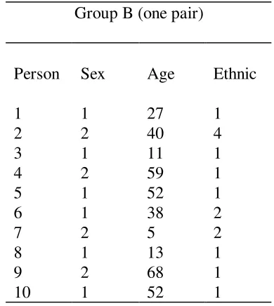
5.1 Some sample data
A worked example on hypothetical data may aid understanding of the
proposed measure. Consider a hypothetical list of individuals, with a few
characteristics. Two lists are used for comparison: group A consists of all
uniques, group B has one pair of ‘twins’; see Table 3. There are three
associated variables, which is the minimum required to be able to define a
set of tables in which one variable is not common across all tables. Four
variables would be required in order to define a set of tables in which it
would be possible to have tables in which the variables do not appear in
any other tables; sex (1-2), age (0-100), and ethnic group (1-4). As the
number of variables in increased, so there is greater flexibility in defining
tables which are linked to other tables to a greater or lesser extent. It is
likely that more realistic results require a larger number of variables but it
is hoped that the small dataset used here will be sufficient to illustrate the
methods used whilst remaining simple enough to follow.
5.2 Measuring disclosure risks in microdata
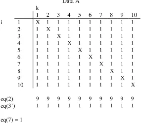
Table 4 shows the Dik tables for Data A and B in full. They are
symmetrical around the i=k diagonal and equations (2) and (3) both require
the full array. The values shows in Table 4 for equation 3’ are a
consequence of equation (3).
∑ −
≠ i ik
ik D N
( 1_ 3’
This indicates some measure of risk for each record. If equation 3’ is
equal to 1, then the record is unique with respect to all other records; if it
is equal to 0 then the record is identical to all other records. In practice it
should be possible to half the computation requirements of filling in the
matrix prior to calculation of these statistics by modifying the formulae
such that only one half of the matrix is required.
Both data sets are small and contain a large proportion of uniques. One
would respect this to be a high risk scenario, and it can be seen that the
value of equation (7) is 1 for group A (the maximum value possible) and
0.97 is the case of group B (a very high value).
5.3 Measuring disclosure risks in aggregate census data
Using the same data, four tables of aggregate census data may be
constructed:
(2) Age & Ethnic group,
(3) Sex & Ethnic group,
(4) Age & Sex & Ethnic group.
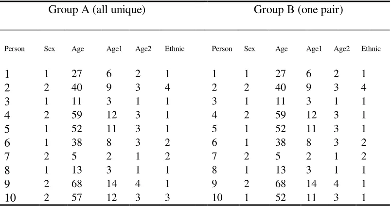
‘Age’ is shown in Table 3 as being single years, but it may be re-coded in
a number of ways; ‘Ethnic Group’ is already assumed to be broad-coded.
The ‘Sex’ variable cannot be re-coded, although it could (as with any of
the three) be replaced by ‘Persons’.
For the purposes of this example, only three tables will be used as being
representative of SAS data. These tables are:
(1) Age & Sex (Age at 5-year groupings, 0-4,5-9,...,90+),
(2) Age & Ethnic group (Age in broad ‘life-stage’ groupings,
0-14,15-29,30-64,65+), and
(3) Sex & Ethnic group.
In all cases, the row variable is quoted first, and it is assumed that cell
numbering is done in a column-then-row pattern.
The table layouts and cell numbers are illustrated in Tables 6, 7 and 8.
In order to avoid complexity at this stage, the broader grouping of ‘age’
has been chosen to have boundaries between classes that are the same as
the 5-year grouping, and to ignore the male-female difference in retirement
Table 5 shows the sample microdata together with the recode values for
the ‘age’ variable.
The data can now be transformed into a 0,1 vector, where each position on
that vector represents a cell in one of the tables produced. The value is set
to 1 if the person is a member of that particular combination of values or 0
otherwise. In this example, the three tables contain respectively 38 cells
(sex=2 by age=19), 16 cells (age=4 by ethnic=4) and 8 cells (sex=2 by
ethnic=4); to give a total length of 62 for the vector of 0, 1 values for each
individual.
Figure (1) shows how the first individual in the sample data would
increment the cross-tabulations, and how those tables would be
transformed to produce the following set of 0, 1 values.
Table 1: 00000000001000000000000000000000000000 Table 2: 0000100000000000
Table 3: 10000000
Person 1: 00000000001000000000000000000000000000 0000100000000000 10000000
The other individuals in group A would produce the following vectors:
Spaces are included to aid readability by separating out the boundaries of
the three tables. The SAS data termed here Ykj is defined as an aggregate
of the above Zij vectors. Assuming that the 10 individuals were the
residents of one ED, then we would get the aggregate vector:
Ykj:
ED total : 00012000001000100100100200010000000000 1100100031111000 41002111
The task now is to compare each of the individuals data profiles with the
aggregate record. Records are considered to be at risk if a 1 in the
individual record matches a 1 in the aggregate record. If the value of any
component of the aggregate record is more than 1, then it indicates that the
corresponding cell in a published table would contain a count greater than
one, and thus it would not be possible to conclusively infer anything about
a particular individual. Each individual record will contain a fixed number
of ‘1’s, depending on the number of tables (or subtables) defined. If each
1 in the individual record matches a 1 in the aggregate record, then that
individual is at risk of being disclosed.
Using the sample data, we can compare the first record with the aggregate
record:
The asterisks identify the locations of ‘1’s in the individual record. It can
be seen that in the final section there is not a match between the individual
record and the aggregate record, and thus the record is not at risk of
disclosing personal details, and thus Dik for this record is 0 (see equation
9).
If this is repeated for the remaining individuals, we find: Dik
Person 2: 00000000000000000100000000000000000000 0000000000010000 00000001 ED total : 00012000001000100100100200010000000000 1100100031111000 41002111
* * * 1
Person 3: 00001000000000000000000000000000000000 0000000010000000 10000000 ED total : 00012000001000100100100200010000000000 1100100031111000 41002111
* * * 0
Person 4: 00000000000000000000000100000000000000 0000000010000000 00001000 ED total : 00012000001000100100100200010000000000 1100100031111000 41002111
* * * 0
Person 5: 00000000000000000000100000000000000000 0000000010000000 10000000 ED total : 00012000001000100100100200010000000000 1100100031111000 41002111
* * * 0
Person 6: 00000000000000100000000000000000000000 0000000001000000 01000000 ED total : 00012000001000100100100200010000000000 1100100031111000 41002111
* * * 1
Person 7: 00010000000000000000000000000000000000 0100000000000000 00000100 ED total : 00012000001000100100100200010000000000 1100100031111000 41002111
* * * 1
Person 8: 00001000000000000000000000000000000000 1000000000000000 10000000 ED total : 00012000001000100100100200010000000000 1100100031111000 41002111
* * * 0
Person 9: 00000000000000000000000000010000000000 0000000000001000 00001000 ED total : 00012000001000100100100200010000000000 1100100031111000 41002111
* * * 0
Person 10: 00000000000000000000000100000000000000 0000000000100000 00000010 ED total : 00012000001000100100100200010000000000 1100100031111000 41002111
* * * 0
The risk of disclosure given by equation (7) is δk k N
N
∑
/ = 3/10 = 0.3Incidentally, using group B, which has two non-unique individuals also
generates a risk of 0.3, however the sample is too small to comment on
what the relationships might be between the proportion of microdata
Thus we find that for this ‘ED’, although all individuals are unique when
considered as microdata, only 3 records are at risk when considered as
SAS or aggregate data. Clearly, much of this reduction of risk is due to
broadcoding of the age variable.
The other significant issue in assessing the risk of disclosure in aggregate
data is the way in which tables are linked by common variables. At one
end of a spectrum, we could imagine a set of tables in which all tables
share a particular variable with common coding standards. If it is possible
to identify an individual given this variable (e.g. if ‘age’ is common, and
there is, say, only one 17 year old in the ED) then it would be possible to
construct an individual record by tracking this person across tables. At the
other end of this spectrum would be a set of tables in which no variable
was used more than once. Clearly, there would be no way to reconstruct
an individual record from these tables, and only partial disclosure could
occur (i.e. we might discover from the tables that there is only one 27 year
old female, and we might also discover that there is only one person who
travels to work by car, but unless there was only one person in the ED
there would be no reason to suppose that these two facts referred to the
same person). In practice, the set of tables will be somewhere between
tables), with a number of different coding schemes. Age and sex are the
obvious common keys.
The question posed is whether or not the proposed method will take into
account the effects of linking tables. If the set of tables contain a large
number of linked tables, then will the proposed method be more likely to
produce a match between an individual and the aggregate record? If two
variables produce a large number of uniques when crosstabulated, then
necessarily the distribution of individuals between categories of at least
one of the variables must include some single counts. If that variable is
used repeatedly (with the same coding) then it seems plausible to suggest
that it will lead to the presence of uniques in other tables in which it is
used, (or at the very least, it will make the presence of uniques more
probable) and that the method will then find more matches.
The possibility of false matches also needs to be considered. For a fixed
number of true matches, if one set of tables generates a large number of
false matches then it implies a lower risk of disclosure. Using the data
previously described above, it can be seen that there are 6 ‘1’s in the first
168 theoretical combinations of ones across all three tables, of which all
but three would be false matches with individuals.
ED total : 00012000001000100100100200010000000000 110010031111000 41002111 * * * * * * ** * **** * ***
The real number of potential matches will be somewhat less than 168,
because of the way that tables are linked. Nevertheless, this high risk of
false matching may well be regarded as an additional disclosure safeguard.
A modification to the method to take false matches into account which
might be introduced is to consider the average risk as defined by equation
(7) compared to the risk of a false match. If such a step was taken, then it
might be useful to take into account the various forms of data modification.
Although the total number of potential matches (i.e. including false
matches) should be calculated using all the (modified) microdata records,
the actual risk should perhaps be calculated only using unmodified Zij
records. This could be achieved by defining some value Xi which would
be set to 0 if a record was unmodified, but set to 1 if the record had been
modified through some pre-tabulation protection method such as record
swapping, or had been introduced to the dataset via imputation. Clearly
such records do not refer to real people, and thus can not be at risk of
disclosure, even if they are FRTUs when the tabulation process is
5.4 Using more tables
The methodology scales up to handle all the SAS cells. Indeed there is a
suspicion that with aggregate census data the risks of disclosure actually
decrease when more cells are used (or at least they do not dramatically
increase as they do in the microdata) because of the increase in
dimensional complex creates a dense fog of uncertainty within which the
probability of a false match is many orders of magnitude greater than that
of a real match. This conjecture can only be proven by computer
experimentation on larger numbers of tables. This work is now underway
funded by the ESRC.
6 Conclusions
The development of an explicit measure of the confidentiality risks implicit
in the release of census data is viewed as extremely useful for the
following reasons:
1.it demonstrates and thus enhances the confidentiality of census data by
ensuring safe release by measuring the actual risks and by applying
consistent standards;
2.it creates the prospect of more useful and flexible census outputs that
census dissemination appropriate for 2001 and beyond with the prospect
of new markets for census data.
The challenge now is three-fold:
1.to complete the research and demonstrate that the statistical assessment
of risk disclosure is viable and works;
2.to demonstrate a prototype system that illustrates the functionality
described here and is proven safe on synthetic data; and then
3.apply the prototype system to real world data in a safe setting and hence
demonstrate to census agencies that the proposals are viable.
Acknowledgement
References
Duke-Williams, O, Rees, P.H, 1997, Can Census Offices publish statistics for more than one small area geography? An analysis of the
differencing problem in statistical disclosure. International Journal of Geographical Information Systems, forthcoming.
Openshaw, S., 1994, ‘Social costs and benefits of the Census’,
Proceedings of XVth International Conference on Data Protection and Privacy Commissioners. Data Protection Registrar,
Manchester. p89-97.
Openshaw, S., (ed), 1995, Census Users’ Handbook. Geoinformation International, Cambridge
Marsh, C., Skinner, C., Arber, S., Penhale, B., Openshaw, S.,
Hobcraft, J., Lievesley, D., Walford, N., 1991, 'The case for samples of anonymised records from the 1991 census,' Journal of the Royal Statistical Society A, 305-340.
Skinner, CJ., Marsh, C., Openshaw, S., Wymer, C., 1990, 'Disclosure avoidance for census microdata in Great Britain', Proceedings
of US Bureau of the Census Annual Research
Conference, US Bureau of the Census, Washington, p131- 143.
Skinner, C., Marsh, C., Openshaw, S., Wymer, C., 1994, 'Disclosure control for census microdata', Journal of Official Statistics 10, 31-51
Table 1 Examples of confidentiality safe aggregate data census outputs
__________________________________________________________
• population and household counts
• an index based on two or more individual variables expressed as an
integer
• a derived statistic computed from several variables; i.e. signed
chi-square
• a set of principal component scores based on 40 variables
• one or more variables recoded as percentages and integerised
• parameters in a statistical model derived from the data
• a multivariate classification cluster code
Table 2 Possible non-census based personal data match keys
__________________________________________________________
gender
age
occupation (broad banded)
house type
tenure
car ownership
Table 3 Synthetic data
Group A (all unique) Group B (one pair)
Person Sex Age Ethnic Person Sex Age Ethnic
1 1 27 1 1 1 27 1
2 2 40 4 2 2 40 4
3 1 11 1 3 1 11 1
4 2 59 1 4 2 59 1
5 1 52 1 5 1 52 1
6 1 38 2 6 1 38 2
7 2 5 2 7 2 5 2
8 1 13 1 8 1 13 1
9 2 68 1 9 2 68 1
Table 4 Dik values for data A and B
Data A k
1 2 3 4 5 6 7 8 9 10
i 1 X 1 1 1 1 1 1 1 1 1
2 1 X 1 1 1 1 1 1 1 1
3 1 1 X 1 1 1 1 1 1 1
4 1 1 1 X 1 1 1 1 1 1
5 1 1 1 1 X 1 1 1 1 1
6 1 1 1 1 1 X 1 1 1 1
7 1 1 1 1 1 1 X 1 1 1
8 1 1 1 1 1 1 1 X 1 1
9 1 1 1 1 1 1 1 1 X 1
10 1 1 1 1 1 1 1 1 1 X
eq(2) 9 9 9 9 9 9 9 9 9 9
eq(3’) 1 1 1 1 1 1 1 1 1 1
eq(7) = 1
Note: Dikis used to measure the similarity of pairs of records: 0 where records are
identical, 1 where they are not.
Data B k
1 2 3 4 5 6 7 8 9 10
i 1 X 1 1 1 1 1 1 1 1 1
2 1 X 1 1 1 1 1 1 1 1
3 1 1 X 1 1 1 1 1 1 1
4 1 1 1 X 1 1 1 1 1 1
5 1 1 1 1 X 1 1 1 1 0
6 1 1 1 1 1 X 1 1 1 1
7 1 1 1 1 1 1 X 1 1 1
8 1 1 1 1 1 1 1 X 1 1
9 1 1 1 1 1 1 1 1 X 1
10 1 1 1 1 0 1 1 1 1 X
eq(2) 9 9 9 9 8 9 9 9 9 8
eq(7) 1 1 1 1 .88 1 1 1 1 1
Table 5 Recoded Microdata
Group A (all unique) Group B (one pair)
Person Sex Age Age1 Age2 Ethnic Person Sex Age Age1 Age2 Ethnic
1 1 27 6 2 1 1 1 27 6 2 1
2 2 40 9 3 4 2 2 40 9 3 4
3 1 11 3 1 1 3 1 11 3 1 1
4 2 59 12 3 1 4 2 59 12 3 1
5 1 52 11 3 1 5 1 52 11 3 1
6 1 38 8 3 2 6 1 38 8 3 2
7 2 5 2 1 2 7 2 5 2 1 2
8 1 13 3 1 1 8 1 13 3 1 1
9 2 68 14 4 1 9 2 68 14 4 1