This is a repository copy of
Route training in mobile robots through system identification
.
White Rose Research Online URL for this paper:
http://eprints.whiterose.ac.uk/74568/
Monograph:
Iglesias, R., Kyriacou, T., Nehmzow, U. et al. (1 more author) (2006) Route training in
mobile robots through system identification. Research Report. ACSE Research Report no.
922 . Automatic Control and Systems Engineering, University of Sheffield
[email protected] https://eprints.whiterose.ac.uk/ Reuse
Unless indicated otherwise, fulltext items are protected by copyright with all rights reserved. The copyright exception in section 29 of the Copyright, Designs and Patents Act 1988 allows the making of a single copy solely for the purpose of non-commercial research or private study within the limits of fair dealing. The publisher or other rights-holder may allow further reproduction and re-use of this version - refer to the White Rose Research Online record for this item. Where records identify the publisher as the copyright holder, users can verify any specific terms of use on the publisher’s website.
Takedown
If you consider content in White Rose Research Online to be in breach of UK law, please notify us by
Route Training in Mobile Robots Through System Identification
R Iglesias
#, T Kyriacou
#, U Nehmzow
#, S A Billings
#Dept Computer Science, University of Essex
Department of Automatic Control and Systems Engineering
The University of Sheffield, Sheffield, S1 3JD, UK
Research Report No. 922
Route training in mobile robotics
through system identification
Roberto Iglesias1
, Theocharis Kyriacou2
, Ulrich Nehmzow2
and Steve Billings3
1
Electronics and Computer Science, University of Santiago de Compostela, Spain.
2
Dept. of Computer Science, University of Essex, UK.
3
Dept. of Automatic Control and Systems Engineering, University of Sheffield, UK.
Abstract. Fundamental sensor-motor couplings form the backbone of most mobile robot control tasks, and often need to be implemented fast, efficiently and nevertheless reliably. Machine learning techniques are therefore often used to obtain the desired sensor-motor competences. In this paper we present an alternative to established machine learn-ing methods such as artificial neural networks, that is very fast, easy to implement, and has the distinct advantage that it generates trans-parent, analysable sensor-motor couplings: system identification through nonlinear polynomial mapping.
This work, which is part of the RobotMODIC project at the universities of Essex and Sheffield, aims to develop a theoretical understanding of the interaction between the robot and its environment. One of the pur-poses of this research is to enable the principled design of robot control programs.
As a first step towards this aim we model the behaviour of the robot, as this emerges from its interaction with the environment, with the NAR-MAX modelling method (Nonlinear, Auto-Regressive, Moving Average models with eXogenous inputs). This method produces explicit poly-nomial functions that can be subsequently analysed using established mathematical methods.
In this paper we demonstrate the fidelity of the obtained NARMAX models in the challenging task of robot route learning; we present a set of experiments in which a Magellan Pro mobile robot was taught to follow four different routes, always using the same mechanism to obtain the required control law.
1
Introduction
1.1 Motivation
The production of robot control code is often a difficult and complex task for the roboticist. Apart from relatively simple behaviours, for example, obstacle avoid-ance or wall-following, tasks such as route learning involve several days or weeks of refining code by trial and error until the robot achieves the desired behaviour. This method of producing code is time consuming and therefore inefficient.
to change the parameters of a task model iteratively, until the model performs within the bounds of an acceptable error. The extent of the training (or model refinement) is usually determined by comparing the performance of the model to that of a validation set of sensor-motor data.
Using artificial neural networks (ANN) is one established approach applied in robot learning. This method speeds up the development of a reactive robot controller significantly; however, it also produces an opaque model that cannot be used to investigate the characteristics of the robot’s behaviour further. Such investigation may include stability analyses, sensitivity of the behaviour to par-ticular sensors or environmental features, sensor redundancy etc. Furthermore, the structure of a neural network model does not allow a straightforward com-parison between models of similar tasks. This is very often necessary in robotic science.
The aim of the RobotMODIC project therefore is to develop a theoretical foundation for robotics. We believe that developing an understanding of robot behaviour will eventually lead to faster, more focused approaches to problem solving.
In this paper we present how we model route learning tasks using the NAR-MAX (Nonlinear, Autoregressive Moving Average models with eXogenous in-puts) system identification process. This process yields explicit polynomial func-tion to represent the task in hand. It is fast and requires no “guess work” as far as the structure or size of the polynomial function that would be suitable for modelling the robot’s task. In addition, there is no need to do any pre-processing of the input space to assist the modelling process. The most important feature of this method, however, is that we can analyse the models obtained using estab-lished mathematical methods in order to understand robot-environment inter-action. Examples of such analyses on previously obtained models and a further discussion of the advantages of the NARMAX modelling procedure for robot tasks such as wall-following and door traversal are presented in [1], [2].
The purpose of this paper is to demonstrate how well the NARMAX models can represent route learning tasks.
1.2 The NARMAX modelling procedure
The NARMAX modelling approach is a parameter estimation methodology for identifying the important model terms and associated parameters of unknown nonlinear dynamic systems. For multiple input, single output noiseless systems this model takes the form:
y(n) =f(u1(n), u1(n−1), u1(n−2),· · ·, u1(n−Nu),
u1(n) 2
, u1(n−1) 2
, u1(n−2) 2
,· · ·, u1(n−Nu)
2 ,
· · ·,
u1(n)l, u1(n−1)l, u1(n−2)l,· · ·, u1(n−Nu)l,
u2(n) 2
, u2(n−1) 2
, u2(n−2) 2
,· · ·, u2(n−Nu)
2 ,
· · ·,
u2(n)l, u2(n−1)l, u2(n−2)l,· · ·, u2(n−Nu)l,
· · ·,
· · ·,
ud(n), ud(n−1), ud(n−2),· · ·, ud(n−Nu),
ud(n)
2
, ud(n−1)
2
, ud(n−2)
2
,· · ·, ud(n−Nu)
2 ,
· · ·,
ud(n)l, ud(n−1)l, ud(n−2)l,· · ·, ud(n−Nu)l,
y(n−1), y(n−2),· · ·, y(n−Ny),
y(n−1)
2
, y(n−2)
2
,· · ·, y(n−Ny)
2 ,
· · ·,
y(n−1)l, y(n−2)l,· · ·, y(n−Ny)l)
were y(n) and u(n) are the sampled output and input signals at time n
respectively, Ny and Nu are the regression orders of the output and input
re-spectively and d is the input dimension. f() is a non-linear function, this is typically taken to be a polynomial or wavelet multi-resolution expansion of the arguments. The degreel of the polynomial is the highest sum of powers in any of its terms.
Noise is always present in physical systems and can be accommodated as part of the NARMAX model. In the present study we have initially assumed that the effects of the noise are small and can be neglected. In later studies the effects of any noise will be accommodated by fitting noise models as part of the identification procedure to ensure that unbiased models are obtained.
The NARMAX methodology breaks the modelling problem into the following steps:
1. Structure detection, 2. Parameter estimation, 3. Model validation, 4. Prediction and 5. Analysis.
These steps form an estimation toolkit that allows the user to build a concise mathematical description of the system. These procedures are now well estab-lished and have been used in many modelling domains [3].
A detailed procedure of how structure detection, parameter estimation and model validation is done is presented in [4]. A brief explanation of these steps is given below.
The initial structure of the NARMAX polynomial is determined by the inputs
u, the output y, the input and output ordersNu andNy respectively and the
degree l of the polynomial. The general rule in choosing suitable inputs for the model is that at least some of them should be causing the output. The number of initial terms of the NARMAX model polynomial can be very large depending on these variables, but not all of them are significant contributors to the computation of the output. In fact most terms, as explained below, are removed from the model equation in the process of refining the model. The final structure of the estimated NARMAX model will indicate any insignificant or redundant inputs.
Before any removal of model terms an equivalentauxiliary modelis computed from the original NARMAX model. The model terms of the auxiliary model are orthogonal. This allows the computation of their associated parameters to be done in a sequential manner, which is computationally very efficient.
The calculation of the auxiliary model parameters and the refinement of the model’s structure is an iterative process. Each iteration involves three steps:
1. Estimation of model parameters (using the estimation data set), 2. Model validation (using the validation data set) and
3. Removal of non-contributing terms.
After the model validation step, if there is no significant error between the model-predicted output and the actual output, non-contributing model terms are removed in order to reduce the size of the polynomial as much as possible. This is primarily done to increase the speed of computation of the model output during its use and also to avoid overfitting the model to the training data.
To determine the contribution of a model term to the output the Error Re-duction Ratio (ERR) [4] is computed for each term. The ERR of a term is the percentage reduction in the total mean-squared error (i.e. the difference between model-predicted and true system output) as a result of including (in the model equation) the term under consideration. The bigger the ERR is, the more signifi-cant the term. Model terms with ERR under a certain threshold (usually around 0.05%) are removed from the model polynomial in the last step of each iteration during the refinement process.
In the following iteration, if the error is higher as a result of the last removal of model terms then these are re-inserted back into the model equation and the model is considered as final. Finally, the NARMAX model parameters are computed from the auxiliary model.
2
Experimental procedure
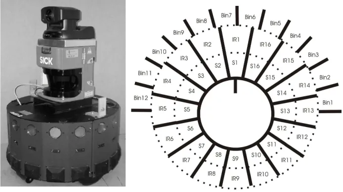
The robot used in our experiments is the Magellan Pro autonomous mobile robot
Radix (figure 1). The robot is equipped with 16 sonar, 16 infra-red and 16 tac-tile sensors distributed uniformly around its circumference. A SICK laser range finder is also present which scans the front semi-circle of the robot ([0◦,180◦])
The robot also incorporates a video camera. In the work presented in this paper only the laser, sonar and infra-red sensors were used.
Fig. 1.Left: Radix, the Magellan Pro robot used in our experiments. Right: Location of each sonar and infrared sensor. The laser sensors have been averaged in twelve sectors of 15 degrees each (laser bins).
During experiments with Radix, the input from all its sensors (apart from the video camera), its position, orientation, transitional and rotational velocities are recorded every 250ms. Position and orientation of the robot are obtained by placing two point-targets on top of the robot and using an overhead video camera to track them continuously. After a logging session the sensor data from the robot and the position/orientation data from the tracking system are aligned using time as the common reference.
Experimental setups of the robot’s static environment are built in a dedicated robot arena usually using carton boxes. Examples of such experimental setups are shown in figures 2, 4, 5 and 6.
In the sections that follow each of the four experiments is presented individ-ually.
2.1 Route 1
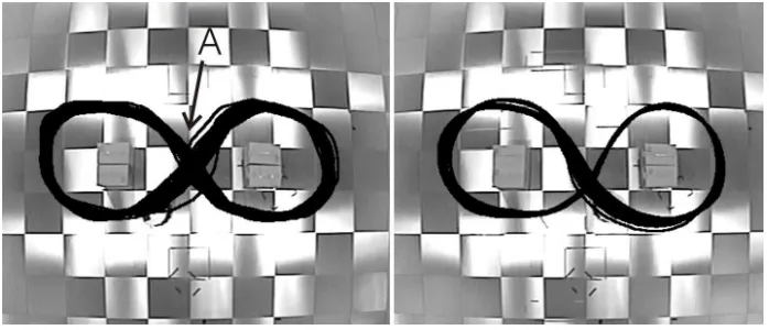
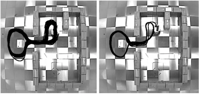
[image:8.612.134.483.270.420.2]The first route the robot had to learn is shown in figure 2. Although this route looks quite simple, it is actually quite difficult to learn because of perceptual aliasing. I.e. the robot’s sensor readings when it is in the middle of the route (labelled A in the graph) are very similar but half of the time the robot has to turn right, while the other half it has to turn left.
Fig. 2.Route 1. Robot trajectory under manual control , used as training data (left), and trajectory taken under model control (right). The model is shown in table 1.
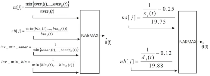
After manual control of the robot along the route for 1 hour, we identified the robot’s movement using a NARMAX process. All the sonar and laser measure-ments were taken into account (figure 3 (left)). The values delivered by the laser scanner were averaged in twelve sectors of 15 degrees each (laser bins), to ob-tain a twelve dimensional vector of laser-distances (figure 1 (right)). These laser bins, as well as the 16 sonar sensor values, were inverted so that large readings indicate close-by objects. Finally, as we can see in figure 3 (left), the sonar and laser readings at each instant were normalised by the minimum sonar and laser reading, respectively, at that instant. These minimum values are also introduced as inputs into the model, so that all the available information is provided. The reason of scaling the inputs is because we saw that the resulting models usually were more robust to small perturbations in the environment.
The parameters of the NARMAX model we obtained are:Nu= 0, Ny = 0,
Ne= 0, degree= 2. The initial model had 496 terms, but after the removal of
Fig. 3. Different ways of providing the laser and sonar information to the modelling strategy. The option shown on the left was used to model robot’s behaviour in routes 1 and 2, while the option shown on the right was used in route 3.
A visual, qualitative inspection of figure 2 is enough to see how closely the robot’s trajectory under NARMAX model control resembles the trajectory ob-tained whenRadixwas manually driven. In order to compare the two trajectories quantitatively as well, we analysed the space occupancy of the two trajectories in (x, y) space, using the Mann-Whitney U-test [5] to determine whether the two trajectories occupy space significantly differently or not. It turns out that the difference between the distribution of values (x−x), when the robot is under
manual control, and the distribution of the same values under NARMAX model control, is not significant (p >0.05). xrepresents the mean of the x-positions. Similarly, there is no significant difference between the distribution of values (y(t)−y) under manual control, and that of the same values under NARMAX
model control, (p >0.05).
2.2 Route 2
Figure 4 shows the second route learnt by the robot through system identifica-tion. This time only the laser sensor was used (pre-processed as it is shown in figure 3 (left) as this produced a better model. The characteristics of the NAR-MAX model obtained in this case areNu= 0,Ny= 0,Ne= 0, anddegree= 3.
The initial model had 573 terms, but just 94 remained after the removal of non-contributing terms.
Figure 4 shows how closely the NARMAX model behaviour resembles the manual control behaviour. Statistical space occupancy tests along thex and y
˙
θ(t) = +0.08−0.50∗nb[1]−0.62∗nb[4] + 0.46∗nb[6] + 0.07∗nb[7]−0.09∗nb[8]+
+0.14∗nb[9] + 0.02∗nb[10] + 0.20∗nb[12]−0.88∗ns[1] + 0.22∗ns[3]−0.04∗ns[5]+ +0.004∗ns[6]−0.04∗ns[7] + 0.20∗ns[10]−0.02∗ns[14] + 0.11∗ns[16]−
−0.43∗inv min bin+ 0.041∗nb[1]2+ 0.02∗nb[2]2−0.06∗nb[3]2+ 0.53∗nb[4]2− −0.44∗nb[6]2
+ 0.01∗nb[9]2
−8.70∗inv min bin2−0.07∗nb[1]∗nb[2]+
+0.07∗nb[1]∗nb[3] + 0.44∗nb[1]∗nb[4] + 0.40∗nb[1]∗nb[10]−0.24∗nb[1]∗nb[11]+ +0.83∗nb[1]∗ns[1] + 0.09∗nb[1]∗ns[4]−0.79∗nb[1]∗ns[11]−0.04∗nb[1]∗ns[13]+ +0.08∗nb[1]∗inv min sonar+ 3.58∗nb[1]∗inv min bin+ 0.36∗nb[2]∗nb[4]−
−0.73∗nb[2]∗nb[9]−0.05∗nb[2]∗nb[12] + 0.04∗nb[2]∗ns[13] + 0.63∗nb[3]∗nb[8]− −0.28∗nb[3]∗nb[12] + 0.11∗nb[3]∗ns[3]−0.48∗nb[4]∗nb[10]−0.27∗nb[5]∗nb[8]+ +0.11∗nb[5]∗ns[1] + 0.26∗nb[6]∗nb[8] + 0.02∗nb[7]∗ns[5] + 0.15∗nb[7]∗ns[6]− −0.18∗nb[7]∗ns[12]−0.17∗nb[8]∗nb[10] + 0.03∗nb[8]∗ns[5]−0.10∗nb[10]∗ns[10]+
+0.05∗nb[10]∗ns[12] + 0.03∗nb[12]∗ns[10] + 0.06∗nb[12]∗ns[11]+
+0.01∗nb[12]∗ns[16] + 2.68∗ns[1]∗ns[6]−0.30∗ns[1]∗ns[11]−1.99∗ns[2]∗ns[6]+
+3.91∗ns[2]∗inv min bin+ 0.13∗ns[3]∗ns[5]−1.27∗ns[3]∗ns[6]−
−1.85∗ns[3]∗inv min bin+ 0.05∗ns[4]∗ns[11]−0.13∗ns[4]∗inv min sonar− −0.23∗ns[6]∗ns[10] + 0.89∗ns[6]∗ns[11] + 0.08∗ns[15]∗ns[16]+
[image:10.612.141.482.382.497.2]+5.06∗ns[16]∗inv min sonar
Table 1.NARMAX model of the angular velocityθ˙for the route
follow-ing behaviour shown in figure 2.nb,ns,inv min sonar, andinv min laser, are the normalised bins, normalised sonar, inverted minimum sonar and laser readings, respectively, shown in figure 3 (left).
Fig. 4.Route 2. Robot trajectory under manual control (left), and, for comparison, under NARMAX model control (right).
2.3 Route 3
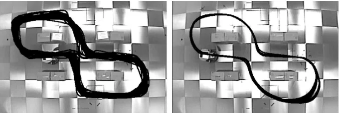
Figure 5 shows the third route the robot had to learn. There are many symme-tries and two narrow passes the robot had to go through. To model the behaviour of the robot along this new route we used the NARMAX strategy once again. To obtain the model, the inverted and normalised laser bins were used (figure 3 (right)).
Fig. 5. Route 3. Robot trajectory under manual control (left), and, for comparison, trajectory of the robot under NARMAX model control (right).
model had 91 terms, but after the removal of the non-contributing ones just 73 remained.
Figure 5 shows the trajectory of the robot during 1 hour when the NAR-MAX model was used to control it. Once again the model was able to properly learn the route in this environment. Apart from the qualitative assessment, this was confirmed using the Mann-Whitney U-test which indicated no significant difference in the space occupancy of the robot (p >0.05) between the trajectory of the robot during manual control and during NARMAX model control.
2.4 Route 4
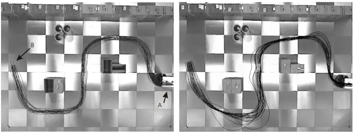
Figure 6 shows a fourth route the robot had to learn. This is an episodic route, which means that the operation of the robot is naturally divided into indepen-dent episodes, each beginning with the robot at position labelled as A in figure 6 and ending in position labelled B.
Fig. 6.Route 4. Left: Robot trajectories under manual control (22 runs, training data), this is an episodic route where each episode comprises the movement of the robot from A to B. Right: Trajectories taken under ARMAX model control (22 runs, test data).
merely done in the previous experiments in order to assist the readability of the model.
In this experiment the regression order of the output (N y) was 0 and that of the inputs (N u) was 8. This means that the model uses a two-second history of sensor inputs.
As shown in figure 6, this model has successfully learned the route from A to B. This is again confirmed using statistical analysis.
3
Conclusions and Future Work
This paper introduces a novel mechanism to program a route following reactive controller through system identification. To obtain the controller, the robot is first operated under human supervision, making it follow a desired route in a specific environment. Once the training data are acquired in this way, we use the NARMAX modelling approach to obtain a model which identifies the coupling between sensory perceptions and motor responses as a non-linear or linear polynomial, respectively. This model is then used to control the robot when it moves autonomously.
Our results confirm that there are cases where the methodology described in this paper is viable. In particular the models we obtained were able to make the robot move properly along the desired routes regardless of the significant perceptual aliasing present in most situations.
paradigms. In the case of artificial neural networks, for example, the nature of the problem would require the use of recurrent architectures.
Finally, it is also very important to consider that a control program obtained through the procedure we propose, is not just an “existence proof”, in the sense that it shows that the robot can achieve a particular behaviour under specific environmental conditions, but it also allows the mathematical analysis of the main factors involved in the robot’s operation in the environment. Thus, the sensitivity analysis of the models obtained, for example, would allow to answer questions related with the importance of every sensor with respect to the robot’s global behaviour, or even to analyse the effect of small perturbations in the environment upon the robot’s operation [6, 1]. The mathematical analysis of these models, and how it can be used to formulate new and testable hypotheses that might lead to a new stage in the experimentation and design of a robot controller, is part of the ongoing research at the universities of Sheffield and Essex.
Acknowledgements
The RobotMODIC project is supported by the Engineering and Physical Sciences Research Council under grant GR/S30955/01. Roberto Iglesias is supported through the research grants PGIDIT04TIC206011PR, TIC2003-09400-C04-03 and TIN2005-03844.
References
1. Theocharis Kyriacou Ulrich Nehmzow, Roberto Iglesias and Stephen A. Billings, “Robot learning through task indentification,” J. Robotics and Autonomous Sys-tems., Accepted.
2. T. Kyriacou, U. Nehmzow, R. Iglesias, and S. Billings, “Cross-platform program-ming through system identification,” inProceedings of TAROS 2005, London, 2005. 3. S. Billings and S. Chen, “The determination of multivariable nonlinear models for dynamical systems,” in Neural Network Systems, Techniques and Applications, C. Leonides, Ed., pp. 231–278. Academic press, 1998.
4. M. Korenberg, S. Billings, Y. P. Liu, and P. J. McIlroy, “Orthogonal parameter estimation algorithm for non-linear stochastic systems,” International Journal of Control, vol. 48, pp. 193–210, 1988.
5. G. W. Snedecor and W. G. Cochran, Statistical Methods, Iowa State Press, 8th edition, 1989.