Massive Model Visualization: A Practical Solution

(1)

2016

Massive Model Visualization: A Practical Solution

Jeremy S. Bennett Iowa State University

Follow this and additional works at:https://lib.dr.iastate.edu/etd

Part of theComputer Engineering Commons,Computer Sciences Commons, and the

Mechanical Engineering Commons

This Dissertation is brought to you for free and open access by the Iowa State University Capstones, Theses and Dissertations at Iowa State University Digital Repository. It has been accepted for inclusion in Graduate Theses and Dissertations by an authorized administrator of Iowa State University Digital Repository. For more information, please [email protected].

Recommended Citation

(2)

Massive Model Visualization: A practical solution

by

Jeremy Scott Bennett

A dissertation submitted to the graduate faculty

in partial fulfillment of the requirements for the degree of

DOCTOR OF PHILOSOPHY

Co-Majors: Human Computer Interaction; Computer Engineering

Program of Study Committee: James H. Oliver, Co-Major Professor Joseph Zambreno, Co-Major Professor

Yan-Bin Jia Rafael Radkowski

Chris Harding

Iowa State University Ames, Iowa

2016

(3)

LIST OF FIGURES

Figure 1: Vertex count in visualization papers [1] ... 1

Figure 2: Performance of traditional LMV approach verses a MMV approach [2] ... 2

Figure 3: Basic MMV System Layout ... 3

Figure 4: MMR viewpoint cell (right) and algorithm (left) [3] ... 8

Figure 5: Far Voxels [11] ... 9

Figure 6: Boeing 777 rendered in real time by Interviews3D [6] ... 11

Figure 7: Single Precession Floating Point Performance for CPU and GPU ... 14

Figure 8: Octree spatial hierarchy ... 16

Figure 9: Multithreaded octree subdivision system ... 17

Figure 10: Octree serialization and extraction time when run on multiple threads ... 18

Figure 11: Visibility Determination Algorithm ... 19

Figure 12: Comparison of MMV and LMV Rendering Frame Rates ... 20

Figure 13: Visibility Determination Algorithm ... 23

Figure 14: LMV verses MMV performance under current system architecture ... 26

Figure 15: Percentage of CPU Time in each Stage for Generation 1 Algorithm ... 27

Figure 16: Percentage of GPU Time Each Stage for Generation 1 Algorithm ... 27

Figure 17: Resulting color buffer for nominal, without quad, and with quad ... 30

Figure 18: GPU Depth Reprojection ... 31

Figure 19: Spatial Hierarchy Buffer Layout ... 34

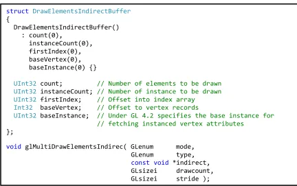
Figure 20: glMultiDrawElementIndirect Specification ... 35

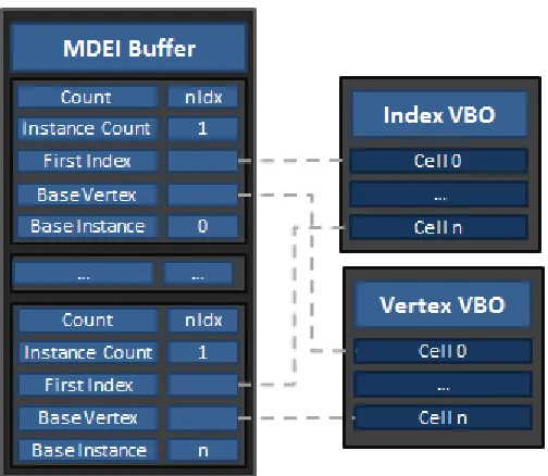
Figure 21: MEDI Buffer Layout ... 36

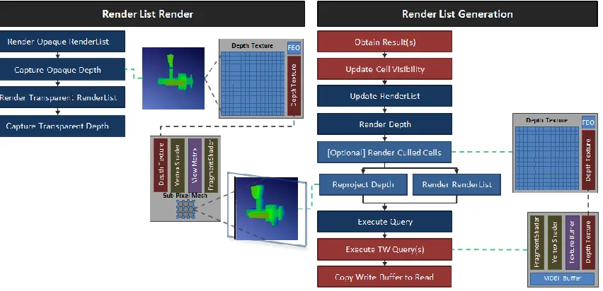
Figure 22: Overview Generation 2 Strategy ... 37

Figure 23: Approximate User Study Scene ... 40

Figure 24: Approximate Path of User Study Animation with Potential Selection Events ... 41

Figure 25: Generation 1 Inside of Geometry ... 44

Figure 26: Generation 2 Oscillation ... 44

Figure 27: Depth Reprojection Plane Z-Fighting ... 45

(7)

Figure 29: Missing Occurrences (Left) and Extra Occurrences (Right) while Rotating 360 ... 49

Figure 30: Reprojected depth buffer blended over the original mesh ... 50

Figure 31: Speed Up When Rendering 360 Degrees Relative to Generation 1 ... 51

Figure 32: Per Frame Performance for the Cotton Picker (Left) and Air Craft (Right) ... 52

Figure 33: Per Frame Render Items for the Cotton Picker (Left) and Air Craft (Right)... 53

Figure 34: Rate of Render Item Change for the Cotton Picker (Left) and Air Craft (Right) ... 53

Figure 35: CPU Performance of Cotton Picker for 360 Degree Rotation ... 54

Figure 36: CPU of Air Craft for 360 Degree Rotation ... 54

Figure 37: User Study Time per Path Key Frame: Overall ... 56

Figure 38: User Study Time per Path Key Frame Event Normalized ... 56

Figure 39: Number of Frames per Path Frame During User Study ... 57

Figure 40: Redraw Time of User Study Path ... 58

Figure 41: Number of Render Items Produced by each Algorithm during User Study ... 59

Figure 42: User Study Path Performance Reprojection 1 ... 60

Figure 43: User Study Path Performance for Reprojection 2 ... 60

Figure 44: User Study Demographic Information ... 62

Figure 45: Question 1 Results (Left) Mean and Confidence Interval (Right) ... 63

(8)

LIST OF TABLES

Table 1: Post Animation Survey ... 39

Table 2: Participant Demographics Survey ... 40

Table 3: Visibility Determination Algorithms ... 41

Table 4: Approaches Used for Testing ... 42

Table 5: Cotton Picker Accuracy ... 46

Table 6: Air Craft Accuracy ... 47

Table 7: Time to Complete User Study Animation ... 55

(9)

ACKNOWLEDGEMENTS

Without the assistance of colleagues, advisors, friends, and most importantly, family,

the present research would not have been possible. I would like to express gratitude to my

major professors and committee members: Dr. James Oliver who has served as both friend and

mentor for more years than I wish to count; Dr. Joseph Zambreno who went above and beyond

expectations to insure I kept one foot in front of the other; Dr. Yan-Bin Jia and Dr. Chris Harding

for their patience and understanding; and finally, Dr. Rafael Radkowski for agreeing to join my

committee at the last moment.

I would like to thank the many colleagues at Siemens PLM Software who have

supported my efforts and served as sounding boards for the many technical questions I faced:

Dr. Michael Carter for serving as both a mentor and a friend; Dr. Adam Faeth who started this

journey with me and has encouraged me along the way; and Tony Deluca, Kevin Glossner, and

Brad Halls for helping me navigate various Siemens’ processes and policies.

I would especially like to thank my friends and family without whose support this would

not have been possible: my wife Audra for her infinite patience and love; my son, Waylen, for

the infinite distractions that helped keep me sane; and lastly, my son, Cassius, for giving me

(10)

ABSTRACT

The ever-increasingly complex designs emanating from various companies are leading to

a data explosion that is far outstripping the growth in computing processing power. The

traditional large model visualization approaches used for rendering these data sets are quickly

becoming insufficient, thus leading to a greater adoption of the new massive model

visualization approaches designed to handle these arbitrarily sized data sets. Most new

approaches utilize GPU occlusion queries that limit the data needed for loading and rendering

to only those which can potentially contribute to the final image. By doing so, these

approaches introduce disocclusion artifacts that often reduce the quality of the resulting

visualization as a camera is maneuvered through the scene. The present research will

demonstrate that shader based depth reprojection and OpenGL atomic writes not only increase

the performance of an existing system based upon OpenGL occlusion queries, but also reduce

(11)

CHAPTER 1. INTRODUCTION

1.1 Motivation

The digital era has promoted the adoption of computer systems throughout an

entire product development lifecycle. Companies are now more capable than ever of

breaking new ground with each successive generation of their products, resulting in

ever increasing complex designs. This, in turn, is leading to a data explosion far

outpacing increases in the processing power of computer systems used to build them,

as shown in Figure 1. The current generation of CAD and Visualization software is no

longer capable of rendering the current generation of airplanes and ships in their

[image:11.612.174.475.332.530.2]

entirety.

Figure 1: Vertex count in visualization papers [1]

The current generation of software is designed around Large Model Visualization

(LMV) technologies. These technologies work by traversing a product structure (usually

represented as a scene graph) and by using various techniques such as view frustum

culling, size culling, occlusion culling, and level of detail representation to limit the

number of polygons rendered when viewing the scene. The problem with this approach

is that it is linear in nature, and therefore computational cost grows at the same rate as

(12)

"Massive Model Visualization" (MMV) is the term used to encompass new

technologies designed to handle this problem. The key principle of MMV is that the

number of polygons that can potentially contribute to a rendered image from a given

viewpoint is limited by the total number of pixels available in the image, not by the total

number of available polygons. A 1080p high definition screen has a resolution of 1920

by 1080, or just over 2 million pixels. If one were to render a relatively large model of

200 million triangles, only 2 percent of those triangles could possibly contribute to the

final image. MMV technologies are about creating a system that is bound by screen

space, not data size, which is definitely not the case with systems based purely on LMV

[image:12.612.128.523.298.530.2]

technologies, as shown in Figure 2.

Figure 2: Performance of traditional LMV approach verses a MMV approach [2]

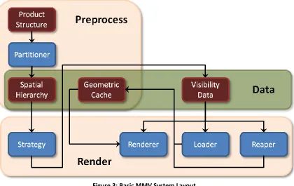
There are several components included in a MMV system that makes this

possible, as shown in Figure 3. As part of a preprocess operation, the product structure

(usually in the form of a scene graph) is subdivided into spatial hierarchy and data

cache. The data cache can contain anything from occurrences, polygons, or voxels,

depending upon the level of subdivision deemed necessary. A strategy pass is executed

during render over the spatial hierarchy in order to construct a visibility list of all data

(13)

renderer to generate the final image, the loader to ensure that any required data is

resident in the geometric cache, and the reaper to ensure that recent unused data is

unloaded from memory. The operations within the render block can be executed in

parallel. The strategy can generate the visibility data for the next frame while the

renderer is still rendering the current frame, and the loader and reaper can run in a

[image:13.612.118.538.218.483.2]

constant cycle, executing data load and unloads as necessary.

Figure 3: Basic MMV System Layout

For a MMV system to be successful, all components must be in place: each plays

a critical role in handling extremely large datasets. The spatial hierarchy generated by

the partitioner must provide enough spatial coherence between the cells for the

strategy to cull large batches of geometry efficiently. The partitioner must also ensure

that the data contained within the cells are sufficiently course to minimize the amount

of noncontributing geometry used. One of the biggest challenges with extremely large

datasets is that they contain vastly more geometric information than the main memory

can manage. Render components must work together to manage the amount of data

resident at any given point in time. The loader is responsible for loading data; it needs to

(14)

predictive algorithms are used by the loader to prefetch likely visible data, minimizing

any potential lag. The reaper is responsible for both detecting and unloading data when

it is no longer necessary, and for determining the best candidates for unloading when

memory approaches maximum threshold. The strategy’s primary responsibility is to

construct a list of visible occurrences. This is accomplished by executing advanced

culling techniques against the spatial hierarchy to determine the set of occurrences

most likely to contribute to the final image. Occlusion tests serve as the primary culling

technique for most approaches.

Culling techniques are not without limitations: they inherently introduce

disocclusion artifacts. Disocclusion artifacts occur whenever a visible shape is not

rendered for one or more frames while visible, thus causing a perceivable popping

effect when finally rendered. This behavior often results from the visibility

determination algorithm’s inability to keep up with the visibility state changes occurring

as the camera is moved through the scene, or if the loader fails to load data before it is

needed.

1.2 Summary of Research

GPU based occlusion tests have been shown to be an effective tool for improving

rendering performance in both industry and games. The present dissertation presents

novel improvements to a GPU based occlusion strategy for improved performance and

reduced disocclusion artifacts. It also presents a simple user study for evaluating how

these improvements affect perceived quality.

1.2.1 GPU Based Depth Buffer Reprojection

GPU based occlusion tests require that the z-buffer be prepopulated with

potential occluders depth values. Most approaches accomplish this by rendering either

a potential occluder list or the existing render list into the depth buffer. On large

models this can involve rendering millions of triangles, far more than the number of

(15)

with Massive Model Visualization techniques is frame-to-frame coherence, or the notion

that the visibility state of occurrences will not change significantly between frames. It

can thus be extrapolated that the zbuffer used for occlusion culling will not alter

significantly. The present research shows how the depth buffer from a previous frame

can be reprojected into the current viewpoint to approximate the current z-buffer using

a textured depth mesh and simple shaders at little cost.

1.2.2 Batch Query

GPU based occlusion strategies frequently rely on GL Occlusion Queries to

determine the visibility of entities. While these provide an easy means for using the

GPU to determine if a given set of primitives will contribute to the final image, they

severely limit the amount of achievable parallelism on the GPU, as entities have to be

queried one at a time. While newer GL extensions have improved upon this

functionality by allowing multiple results to be retrieved simultaneously, it still comes at

significant cost.

GPU based Atomic Increment has been shown to be a viable alternative to GPU

Occlusion Queries, allowing the visibility of all entities of interest to be obtained with a

single draw call, thereby significantly increasing GPU parallelism. The present research

shows how this can be effectively combined with spatial hierarchy to increase its

scalability to arbitrarily large data sets.

1.2.3 User Study Perceived Quality

A common side effect of occlusion based culling techniques is the popping in and

out geometry as it transitions between visible and invisible states. These disocclusion

artifacts can have a severe impact on the perceived quality of the rendered image. This

research also presents an evaluation of how novel improvements affect perceived

quality through the execution of a simple user study.

(16)

1.3 Dissertation Organization

The remaining chapters of this dissertation will provide the necessary

background and implementation details for the executed research. Chapter 2 will

present the current research trends in Massive Model Visualization. Chapter 3 will

provide the high-level system architecture enhanced as part of this research. Chapter 4

will provide a detailed description of how frame-to-frame coherence can be applied to

depth buffer generation. Chapter 5 will show how shader buffer write and multi draw

instance indirect can be combined with existing spatial hierarchy to form a substantially

better query algorithm capable of querying the entire spatial tree in a single call.

Chapter 6 will present the user study used to evaluate the effects of disocclusion

artifacts on perceived quality. Chapter 7 will provide detailed results of novel

improvements and how they compare to the original algorithm. Chapter 8 will provide

(17)

CHAPTER 2. RELATED WORK

Over the last several years there has been a wide array of approaches to

achieving interactive framerates on arbitrary large models. While the scope and

complexity of systems vary greatly, they are all built on the foundation of using

occlusion queries to significantly reduce the amount of data required for rendering.

Several systems and approaches will be introduced below to further describe the scope

of the problem.

2.1 MMR

MMR, Massive Model Rendering, was designed and implemented as part of the

Walkthru Project at the University of North Carolina in Chapel Hill. Like Interviews 3D,

its developers realized that CAD model sizes are increasing at a much faster rate than

the rendering capability of commodity hardware. A new approach was needed to

render these Massive Models containing more than 1 million primitives at interactive

framerates of 20 frames per second or more. MMR was built from the ground up to be

an extensible platform for enabling further research into arbitrarily large models that

can easily scale with model size. Its design allows researchers to interchange various

techniques while processing these massive models.

The basic strategy employed by MMR is to avoid rendering any geometry the

user will not see, and it is facilitated by a two-part technique. The first part eliminates

any geometry that is far away from the viewer by using an image replacement

technique. The second part optimizes the rendering of nearby geometry through

common acceleration techniques such as occlusion culling and level-of-detail. Input

(18)

Figure 4: MMR viewpoint cell (right) and algorithm (left) [3]

The image replacement technique replaces faraway objects with textured depth

meshes. The model space is sub-divided into a set of viewpoint cells using a view

emphasis function to determine which objects are considered far from the viewpoint.

The view emphasis function is a user-defined function that is unique for each model,

returning a scalar importance measure for any point in the model space that allows for

the area importance to be easily determined. Each viewpoint cell is given a large cull

box that may overlap with neighboring cell cull boxes. Objects outside a cell's cull box

are considered far from the viewer when standing inside the cell. A set of depth maps

are created for each view point cell and contains resulting color and depth values for the

geometry outside the cull box when looking from the center of the cell through each of

its sides. This data is used to generate a simplified texture depth mesh for each side

that can serve as a necessary stand-in using algorithms from Darsa and Sillion for heavy

reductions in complexity, and Garland and Heckbert for fine tuning reductions [4, 5, 6].

Each object is processed so that large objects intersecting multiple viewpoint

cells can be split into sets of smaller objects, thereby facilitating the use of techniques

required to render near-geometry. Further, alternate representations are created for

each object using a minor variation of a method proposed by Erikson and Manocha [7].

Last, potential occluder objects are calculated for each cell.

MMR uses a four-process approach to handle renderings of arbitrarily large

models. The main process is devoted to rendering and handling operations occurring

(19)

devoted solely to occlusion culling. The last process handles asynchronous I/O and

attempts to pre-fetch any texture depth maps or tri-strips needed in subsequent frames

[8, 9, 10].

2.2 Far Voxels

Far Voxels is a volumetric approach for rendering arbitrarily large models.

Realizing that model size is quickly outpacing the graphics capability of most commodity

hardware, Gobetti and Marton set out to create a method that will work on a larger

subset of models that is better than currently available output-sensitive approaches.

Figure 5: Far Voxels [11]

Gobbetti and Marton’s approach uses a pre-processing step to generate a coarse

volume hierarchy whose leaf nodes contain a fixed number of triangles, and interior

nodes contain a voxel approximation of underlying nodes. The hierarchy is generated

by using the surface heuristic approach, as defined by MacDonald and Booth, to

sub-divide the model into an axis-aligned BSP tree [8], and the resulting tree is stored in

memory coherent order to improve cache locality, similar to one proposed by Harvan

[9]. Once complete, the tree is combined with a coarse hierarchical data structure by

first removing empty nodes, and then associating sub-trees containing a set number of

BSP tree triangles to leaf nodes in the hierarchy. The hierarchy is traversed to finalize

each leaf node, and immediately saved out to disk once the data structures have been

(20)

culling out triangles outside the nodes bounding box, tri-striping resulting triangles, and

performing optimizations to increase cache coherency of the resulting data. The

interior nodes view-dependent voxels are generated by casting a large random set of

rays against the BSP tree at each node to generate a set of pixel samples from

approximately all un-occluded directions. These samples are then fitted to a set of

shader models to compress their size and allow for more efficient rendering. The input

data set is split into chunks containing between 20 and 30 million triangles to take

advantage of the massive parallelism that exists within the subdivision approach. These

chunks are then farmed out to a networked group of computers that generate a tree for

the model’s respective section.

Rendering occurs in breadth-first, front-to-back order on a set of trees. A

priority queue is used to sort the current set of nodes to be potentially rendered in a

front-to-back order, with the initial set of nodes for each frame being the root nodes of

all trees. While there are still nodes in the queue, the front node is removed and

processed for rendering. All nodes are initially marked as invisible in the current frame,

so during processing the active node can simply be discarded, resulting in it and its

whole sub-tree being culled from the current frame. For example, if the active node's

bounding box is completely outside the view frustum, it is discarded without going

through the occlusion query machinery. The occlusion query machinery handles each

node based upon the node’s state. Nodes that were invisible in the previous frame are

initially queried against their bounding box. Leaf nodes determined to be below a

certain screen coverage threshold, and nodes with children not yet loaded, are queried

against their actual render. For all other nodes, their children are pushed directly into

the potentially-render queue. The occlusion results are handled once they become

available, and nodes whose queries result in zero visible pixels are immediately

discarded. All other nodes, and their ancestors, are marked as visible and their children

are pushed into the queue. Further, any node whose bounding box was rendered is

(21)

queries, the node associated with the top-most query is handled without waiting on the

query to complete.

The loading of nodes is handled through an asynchronous I/O mechanism, and

the list of nodes to be loaded is processed at each frame. Fetch requests are issued for

as many nodes as can possibly be handled in a given amount of time. Nodes are

pre-sorted based upon the estimated voxel size of their parent in order to give a higher

priority to nodes that will potentially contribute to a much larger region of the screen

[11].

2.3 Interviews3D

One of the most complete systems available for Massive Model Visualization is

Interviews3D, supporting navigation, picking, manipulation, animation, and even

collision detection. It is described by its creators, 3D Interactive, as a digital mockup

system capable of handling data sets with millions, if not billions, of triangles on

commodity hardware by using a visibility-guided rendering approach.

Figure 6: Boeing 777 rendered in real time by Interviews3D [6]

Interviews3D was built around a set of pre-defined principles that helped guide

and influence its development. The key principles that all systems can utilize include: (a)

determine rendering performance by output complexity instead of data size, (b) load

and unload data automatically, and allow it to exist in memory only when needed, (c)

exploit temporal coherence between frames whenever possible, (d) update rather than

(22)

In order to efficiently handle the visualization of arbitrary large models,

Interviews 3D uses a preprocessing step to generate an axis-aligned bounding box tree

out of input data through a top down approach, resulting in leaf cells containing

between 1000 and 8000 triangles. The exact algorithm used for subdivision is not

provided, however some key features are explicitly stated. The resulting tree can be

selectively updated based upon changes in the original data set, which is significantly

more efficient than rebuilding the whole tree. Available memory is taken into account

when processing the tree, and if necessary, a multi-pass approach that works only on a

subset of the input data is used. Bounding boxes are kept as uniform in size as possible

while splitting the side lengths of a cell. Individual triangles are never split or

duplicated, meaning there may be some overlap between the bounding boxes of child

cells. Subdivision is based upon a minimum number of polygons in a given cell and is

calculated for the whole input data set based upon a variety of factors.

The use of spatial hierarchy allows Interviews3D to achieve an interactive

framerate through the use of nothing more than an occlusion algorithm and a simple

LOD mechanism. The occlusion algorithm is very similar to the one presented in GPU

Gems 2, making full use of the GPU capabilities of its time and taking into account the

temporal coherence in the geometry rendered from one frame to the next [12]. In

order to do this, each cell in the spatial hierarchy is labeled “visible”, “invisible”, or

“untested.” Rendering uses these states to carry out a two-pass rendering approach. In

the first pass, all shapes marked as “visible” are rendered to prime the depth buffer for

occlusion queries. In the second pass, the tree is recursively traversed in a

front-to-back, top-down manner using standard view frustum and occlusion tests. When a cell

labeled as “invisible” or “untested” is encountered, an occlusion query is immediately

executed and the traversal is pruned. Obtaining the results of each occlusion query

occurs in parallel to the tree traversal in order to prevent stalls in the graphics pipeline.

A post-render tree traversal propagates the visibility state up the graph. A simple LOD

mechanism determines the cells that would contribute a pixel or less when rendered to

(23)

Data management occurs asynchronously within Interviews3D and is coupled

tightly with the rendering approach. The main objective is to load as many leaf cells as

possible into memory, based upon their priority order (respectively, from highest to

lowest: visible, invisible but within view frustum, invisible, and finally single-pixel cells).

If cells should need to be removed from memory, the cells with lowest priority are

removed first, based upon which cell has been in memory the longest[2, 6].

2.4 CPU Based Culling

Coverage buffer culling covers the new class of CPU based occlusion culling

techniques that have become popular among major gaming engines. The primary goal

of coverage buffer culling is to shift visibility culling back to the CPU to devote all GPU

resources toward rendering and achieving ultra-realism at consistently high frame rates.

The steady increase in available cores has made it possible to execute complex culling

techniques on the CPU with limited to no-impact on other operations. The basic

premise of coverage buffer culling is to execute a software rasterisation of simplified

objects such as bounding boxes that are then tested against a depth buffer to determine

visibility.

FrostBite 2 by dice accomplishes the above by rasterizing a course depth buffer

using low polygon occluder meshes. The depth buffer can then be used to cull all

objects by executing a screen space test [13]. CryENGINE 3 by CryTek reads the

previous frame’s depth buffer back from the GPU to the CPU after executing a

down-scaling pass on the GPU. On consoles such as the Xbox 360 and the PS3 this can be

accomplished with only 1 frame of latency, however on a PC this can take up to 4

frames. A course rasterisation of objects AABBs and OBBs are used for calculating

visibility on a separate CPU thread. The problem with this solution is that there can be a

significant difference in the depth buffer from the previous and current view-point

resulting in invalid visibility results. The above problem is solved by executing CPU side

(24)

buffer from the GPU. A 3x3 dilation pass is used in an attempt to stich any holes that

may have opened up as a result of the reprojection [14, 15].

2.5 GPU Based Culling

Figure 7: Single Precession Floating Point Performance for CPU and GPU

With GPU performance gains far outpacing those of the CPU, there is interest in

shifting the entire culling process to the GPU. Tavenrath and Kubisch, researchers from

the NVidia SceniX Team, presented a prototype for an advance scene graph rendering

pipeline at the GPU Technology Conference (GTC) in 2013. They defined four key points

for getting the most out of a render list render. First, the pipeline should share as much

geometry as possible. Second, all input parameters should be grouped for fast

updating. Third, use MultiDrawIndirect to increase GPU batch size and minimize the

number of draw calls. Finally, use the NVidia bindless extension: it provides more

flexibility and allows for some of the validation to be bypassed. They also detailed a

four-stage culling approach. In the first stage, the previous render list is rendered fully

shaded. In the second stage, the entire list of occurrences is tested against the current

depth. In the third stage, any newly visible objects are rendered. In the fourth and final

stage, update the render list to contain only objects that are visible in this frame. The

occlusion test renders the 3 visible sides of the bounding box in the geometry shader,

uses the existing depth buffer to perform early z-cull on invisible fragments, and uses

(25)

At SIGGRAPH 2015 in Los Angles, Haar and Aaltonen presented a talk about the

GPU Driven Rendering Pipeline of Assassin’s Creed Unity. Designed for the latest

generation of hardware, the game saw a massive increase in the amount of geometry to

be rendered. For any given scene, rendering individual components would easily result

in over 50000 draw calls, almost 10x the desired number. To combat this, they use a

mesh cluster rendering approach to improve both batching and culling granularity. The

basic principle is to partition all geometry into fixed sized clusters of triangles. This

allows glMultiDrawIndexedInstancedIndirect to be used to draw and easily cull an

arbitrary number of clusters. Their basic rendering algorithm follows an 8-stage

approach with a majority of the work offloaded to the GPU. Stage 1 consisted of a

course frustum culling algorithm, stage 2 was responsible for updating all GPU data, and

stage 3 batched the draw calls. Starting with stage 4, all work was executed on the GPU

beginning with instance culling that utilizes a quad tree based occlusion culler. Stage 5

executed a cluster chunk expansion, while stage 6 executed cluster culling using

frustum, occlusion, and backface based techniques. Stage 7 was responsible for

generating and compacting the index buffer. Finally, stage 8 executed the scene render.

The zbuffer for occlusion testing is generated using a multi-pass process. The first pass

renders the best occluders at full resolution, the second pass-down samples the

resulting depth buffer, the third pass combines this depth buffer with a low resolution

reprojection of the last frame, and the fourth and final pass generates a depth hierarchy

for more efficient GPU culling [17].

2.6 Massive Model Visualization:

An Investigation into Spatial Hierarchies

In order to develop a complete Massive Mode Visualization solution one must

have a solid understanding of the numerous technologies and techniques, and how they

are used to accelerate the various sub-components of the system. To this end, a

prototype was developed to explore how a spatial hierarchy combined with a visibility

determination algorithm can be used to accelerate rendering performance on arbitrarily

(26)

2.6.1 Spatial Hierarchy

The spatial hierarchy for the prototype placed a strong emphasis on minimizing

the size of individual cells in order to lower the potential L2 cache impact when

traversing the tree. The cells were formed into an octree, as shown in Figure 8, because

the uniform subdivision allowed for bounding volume information to be calculated

dynamically for each cell based upon the path taken to reach the cell, rather than having

to be stored. This, combined with other optimizations to limit the amount of state that

must be stored, resulted in each cell requiring at most 48 bytes.

Figure 8: Octree spatial hierarchy

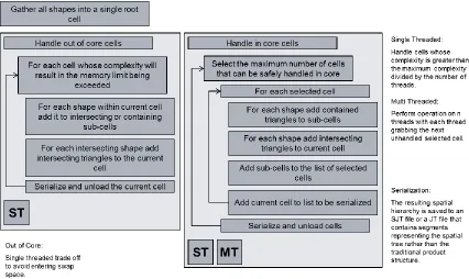
As shown in Figure 9, each octree is generated by harvesting the bounding

volume information for all occurrences in an assembly extracted from a set of ISO

standard Jt files, and subsequently feeding this information into a system for subdividing

the tree on multiple threads while minimizing memory usage. The system starts by

placing all occurrences on the root cell and then placing it in the queue to be

subdivided. The queue is then traversed in order, subdividing any cells that are

considered too large to be handled in system memory and subdividing large cells to

ensure queue length is sufficient to be handled by multiple threads. Once complete,

additional threads are launched and the cell queue is processed as though each entry is

the root cell of another spatial hierarchy. The results are then inserted back into the

(27)

cell that contains them. Occurrences that intersect multiple child cells are subsequently

loaded, and their triangles, along with those pushed down from higher level cells, are

added to any child cell that contains them, otherwise they are left on the current cell.

Lastly, the cell is serialized to a file and its data are unloaded to conserve memory. Cells

are subdivided only if their complexity is greater than a sentinel value of usually 5000

triangles. If the cell does not meet the criteria to be subdivided, its occurrences are

loaded, and its triangles are added to the triangle bucket on the cell, serialized and

[image:27.612.108.534.257.511.2]

unloaded.

Figure 9: Multithreaded octree subdivision system

The performance of the spatial hierarchy subdivision algorithm was measured by

executing the process on the same data set using an increasing number of threads. The

algorithm achieved impressive gains for both extraction and serialization when two

threads were used, as shown in Figure 10. However, decreases in the extraction time

quickly tapered off and no gains were seen beyond five threads, whereas serialization

(28)

Figure 10: Octree serialization and extraction time when run on multiple threads

2.6.2 Visibility Determination Algorithm

The algorithm presented in GPU Gems was combined with the algorithm

described by 3D Interactive to create a hybrid approach and determine the visibility of

cells. Both algorithms focus on rendering only occurrences that can potentially

contribute to the final image, while trying to ensure that GPU occlusion queries are

interleaved with visible cell renders in order to minimize system stalls when retrieving

occlusion query results.

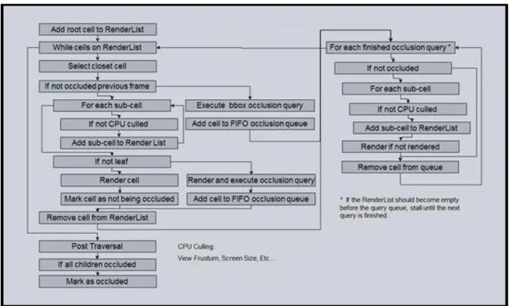
As shown in Figure 11, the algorithm starts by pushing the root cell into a heap

that is sorted based upon distance from the viewpoint, and then traversing through the

heap by popping the nearest cell. If the cell were considered occluded in the previous

frame, an occlusion query is executed by testing the cell’s bounding volume against the

depth buffer and pushing the cell number and occlusion id into a FIFO queue of

outstanding queries. If the cell were not considered occluded in the previous frame,

and it is a leaf, an occlusion query is executed by rendering the cell into both the color

and depth buffer and pushing the cell number and occlusion id in the queue of

outstanding queries. If the cell were not considered occluded in the previous frame

and it contains children, it is rendered into both the color and depth buffers and its

children cells are inserted into the heap if they pass a series of CPU based occlusion

(29)

query queue is checked every 10 cells to determine if the head entry is ready, and if it is,

its pixel count is retrieved from the GPU. If the value is less than 5 the cell associated

with the entry is marked as occluded. If the value is greater than, or equal to 5 it is

marked as not occluded, and if it were previously marked as an occluded cell, it is

reprocessed as though it were visible. This process is repeated for all entries that are

ready. After both the heap and queue are empty, a depth first traversal is executed

[image:29.612.140.508.233.454.2]

over all visible cells, marking any cell whose children are culled as occluded.

Figure 11: Visibility Determination Algorithm

Testing showed this hybrid approach was able to achieve significant gains over the

traditional LMV approach, as seen in Figure 12. While it was not able to achieve the

smooth curve that one would expect from an algorithm that was truly bounded only by

(30)

Figure 12: Comparison of MMV and LMV Rendering Frame Rates

2.6.3 Results

The prototype was able to successfully validate the capabilities of MMV

technologies and how they could potentially be used to accelerate commercialized

visualization software.

The spatial partitioner demonstrated that the extraction and serialization of a

product structure based JT file into an octree based spatial hierarchy can be effectively

executed in a parallel fashion, however, it still left a lot to be desired in terms of overall

performance and memory usage. While it was able to extract the 777 into an octree, it

required that the process be run for approximately 12 hours overnight on a machine

with over 24 GB of ram. The octree based spatial hierarchy provided a uniform spatial

subdivision of triangles that worked well to demonstrate the benefits of GPU based

occlusion culling. However, the uniform subdivision did not take into account the

natural divisions within the model, and therefore, did not provide ideal spatial

subdivision. The handling of large triangles fell short of expectations. Leaving them on

higher-level cells resulted in a considerable amount of geometry being left too high in

the spatial hierarchy and reduced its efficiency, while pushing them down into children

cells resulted in far too much triangle duplication. Further, the actual splitting of

(31)

(PDM) models and does not allow for on-the-fly configuration, or provide an easy means

by which data access can be limited.

The spatial renderer showed that visibility guided rendering techniques have the

potential to easily double previously established frame rates. It also showed that

proposed algorithms have weaknesses. While the interleaving of cell rendering and

occlusion query helps minimize stalls, it only works as long as there are cells available

for rendering. The active cell heap became empty frequently, resulting in pipeline stalls

while the renderer waited on occlusion results to become available. Interleaving ensures

that visibility changes are reflected quickly (the algorithm will continue traversing until

the complete visibility state is known,) however, this can lead to inconsistent frame

rates, especially when the visibility of large sections of the spatial tree changes.

Interleaving doesn’t readily separate render list render from render list generation, thus

(32)

CHAPTER 3. SYSTEM ARCHITECTURE

The prototype proved that massive model technologies can significantly increase

performance by rendering only triangles that are likely to contribute to the final image.

However, its design left a lot to be desired, especially if it is to be integrated into an

existing Computer Aided Drafting (CAD) or Engineering Visualization product. A formal

project was executed as part of the Teamcenter Visualization 10.1 development cycle to

adapt the prototype system developed as part of my master thesis to a system that will

work directly against data stored in a Teamcenter Product Data Management (PDM)

System. This work resulted in a new Spatial Hierarchy (SH) Design as well as a complete

refactor in the Visual Determination Algorithm (VDA).

3.1 Spatial Hierarchy Design

The new spatial hierarchy is based on a bounding volume hierarchy over

occurrences. Each cell within the tree contains its bounding volume information,

occurrences, and children cells. The same occurrence can appear in multiple cells and

occurrences contained within a cell can be dynamically determined at run time. No

specific algorithm is currently required for partitioning of the spatial hierarchy, however

several were implemented: Median Cut, Octree-Hilbert, and Outside-In.

The bounding volume over occurrence allows the visibility state of a given cell to

be directly translated to the visibility state of an occurrence, and also allows the

occurrences contained within a given cell to be dynamically configured as cells become

visible. Both features are critical for integrating directly against a PDM and enabling

visibility guided interaction. A spatial hierarchy over occurrences is severely limited in

how it can spatially subdivide the model; the spatial hierarchy was updated to support

the same occurrence in multiple cells to compensate for this, allowing for a better

subdivision while still allowing for cell visibility to be traced back to individual

occurrences. This also has the potential of enabling sub part culling in future versions

(33)

A query representation is dynamically generated for each cell at run time. This

allows for the representation to be matched to the visibility determination algorithm

used. For example, a set of triangles representing the bounding volume is generated

with OpenGL occlusion queries.

3.2 Visibility Determination Algorithm

For any MMV solution to be viable it needs to limit the amount of data that is

both loaded and rendered when viewing a scene. The visibility guided rendering

algorithm first introduced in GPU Gems and further enhanced by Interviews3D performs

well in determining the visibility of occurrences, and therefore limits the amount of data

needed to be loaded. However, these algorithms run the risk of stalling the GPU if there

are insufficient visible cells to avoid waiting for an occlusion query to complete. Worse,

the interleaving of visibility determination with rendering makes it impossible to switch

out the visibility determination algorithm or make full use of multi core or multi GPU

systems. In order to get around these limitations, the visibility determination algorithm

has been split into two pieces: Render List Generation and Render List Render.

(34)

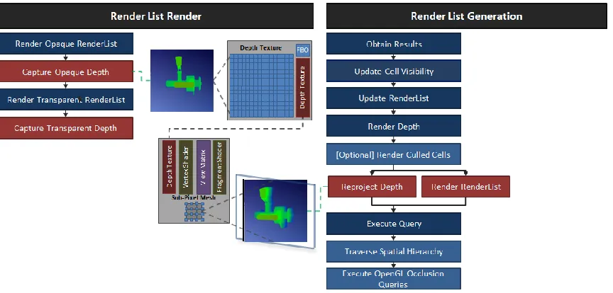
3.2.1 Render List Generation

Render list generation utilizes a visibility determination algorithm to create a list

of all occurrences and their associated state that are likely to contribute to the current

image. This is divided into five distinct stages under the current system architecture:

Obtain Results, Update Culling, Update Lists, Render Depth, and Execute Query.

3.2.1.1 Obtain Results

During the obtain results stage the outstanding query list is traversed, and for all

queries that are ready, the number of pixels that were hit during rendering are obtained

from OpenGL. If the number of pixels is greater than the visibility threshold, the

associated cell is marked as visible. The pixel value is also used to set the number of

frames each cell should delay before executing another query. Frame delays for queries

were introduced as a means to reduce the number of queries executed in a given frame.

Originally these delays were set to a fixed value, however later research showed that a

random delay is actually better at producing a more even spread [18]. The above logic

aims for a middle ground in which cell queries are spread out: cells that are more likely

to change visibility state are queried more frequently.

3.2.1.2 Update Culling

During the update culling stage tree cells are traversed, starting at the front and

progressing up to the tree’s root cell. Any cell not contributing enough pixels to the

current frame is marked as culled, and any cell whose children are all culled is marked

potentially culled.

3.2.1.3 Update Lists

During the update lists stage the visibility value for all occurrences is initially set

to 0. The tree is then traversed such that the pixels value for all visible cells can be

propagated to their contained occurrences. The largest pixel value is used if an

occurrence is referenced by multiple visible cells. Once traversal is complete, all

(35)

render list with the level of detail selection for a particular occurrence based on its pixel

value. The resulting render list is then sorted based upon material properties to

minimize the amount of state changes that must occur whenever it is rendered.

3.2.1.4 Render Depth

During the render depth stage the render list from the previous frame is

rendered slightly offset back into the depth buffer in order to initialize it for executing

GPU based occlusion queries. The bound state during rendering is limited to only that

state that can potentially influence the depth buffer results. Further transparent

occurrences are ignored, as they are not likely to cause other occurrences to be

completely occluded.

3.2.1.5 Execute Query

During the query execution stage the spatial hierarchy is traversed in a depth

first order starting with the set of seed cells that are contained within the view frustum

and moving all the way down to the visibility front. Each cell that is traversed loads its

occurrence information if it is not already resident or is marked as invalid, determines if

its children should be traversed, and if so inserts any that are not view frustum culled

into the active cell heap, and finally executes the query action. Children cell loading and

query actions are selected by combining relevant state to form an index value that can

then be used to lookup the desired action from a carefully constructed table.

3.2.2 Render List Render

Render list render renders the list of all visible occurrence as efficiently as

possible. The data structure was designed to utilize modern GPU functionality while

minimizing the potential L2 cache impact. The current implementation is based around

rendering unified vertex buffer objects (VBOs) (multiple shapes in the same buffer) with

(36)

3.3 Baseline Performance

The performance of this system architecture was established by comparing the

MMV rendering time to the time taken by the original LMV based approach using the

same data. On average, the system is able to achieve approximately a 2x increase in

performance, as seen in Figure 14, which is in line with the prototype; however, it is still

far from achieving the desired results.

Figure 14: LMV verses MMV performance under current system architecture

Taking a closer look at the individual stages for two particular models, as shown

in Figure 15, one can see that the CPU time is primarily dominated by the stages

associated with the visibility determination algorithm. For the aircraft, over 72 percent

of CPU time is spent in strategy. Of this, 24 percent of the time is spent populating the

render list, 22 percent retrieving the results back from GL, 9.9 percent executing the

OpenGL occlusion queries, and 7.2 percent traversing the spatial hierarchy to determine

what cells need to be queried. For the cotton picker, over 80 percent of the CPU time

was spent in strategy. Of this, over 31 percent is spent executing the OpenGL occlusion

queries, 20 percent is spent populating the render list, and 14 percent is spent

traversing the spatial hierarchy. The traversal, query, and result stages are all bound by

the current visibility determination algorithm and could potentially be optimized by

(37)

a render list from the current visibility information and is likely to see performance gains

only by decreasing the number of occurrences marked as visible.

Figure 15: Percentage of CPU Time in each Stage for Generation 1 Algorithm

The GPU Time, shown in Figure 16, shows a wide variation between models. For

the aircraft dataset only 35 percent of the time was spent executing the VDA and of

that, over 25 percent was spent populating the depth buffer by rendering the previous

render list. For the cotton picker dataset, almost 75 percent of the time was spent

executing the VDA, however the depth buffer population was a mere 5 percent.

Executing OpenGL occlusion queries and generating the MDEI buffers dominated with

30 percent of the time each. This shows that as model size increases, the GPU time is

bound stronger by what is rendered than the VDA used to determine what is to be

rendered. Some performance gain can be appreciated by improving the depth

population; however, a majority of the gains are likely to be achieved by only reducing

the amount of geometry rendered by the render list.

(38)

CHAPTER 4. GPU DEPTH REPROJECTION

This Computer Engineering and Human Computer Interaction Research

demonstrates a GPU based approach for reprojecting the depth buffer from one view

into another in order to accelerate GPU occlusion queries by exploiting the natural

frame to frame coherency in the depth buffer.

A key principle of most modern day MMV solutions is frame-to-frame coherency,

or the concept that a visible set of occurrences is not likely to change considerably

between adjacent render frames. This principle serves as the backbone upon which

most culling techniques are based: it allows a set of occurrences to be minimized when

each frame needs to be tested, especially when combined with an acceleration data

structure such as a spatial hierarchy. The same principle can be applied to depth

information required for executing occlusion queries, as the depth buffer is also not

likely to change significantly between frames. While some approaches have begun to

utilize this concept, none are designed to operate purely on the GPU.

Early MMV approaches found that the depth buffer can be used to generate

higher fidelity alternative representations such as texture depth meshes, and it can be

used as either stand-ins for particular occurrences [19, 20, 21] or faces of a particular

view cell [22, 3, 23, 24, 25]. This allowed system performance to be increased by

significantly reducing the number of polygons rendered for each frame at the cost of an

expensive preprocessing step that might not be amenable to all applications.

Modern game engines utilize depth buffer approximations to accelerate their

visibility determination algorithms. Frostbite developed by DICE uses the CPU to

rasterize a course zbuffer on the CPU, based upon at most 10,000 vertices worth of low

polygon count occluder meshes, which is then used to cull objects in the scene using a

screen space bounding box test [13]. In a similar fashion, CryENGINE 3 by Crytek

generates a depth buffer approximation and then uses hierarchical occlusion culling to

(39)

object oriented bounding boxes on the CPU. The approximation is generated by using a

software rasterizer to generate a depth buffer on a PC. On the console they were able

to retrieve the depth buffer from 2 to 3 prior frames. The depth buffer was reprojected

into the current view to improve the quality of the occlusion tests, and a dither

operation was used to close some of the gaps [14].

Depth information is often populated by rendering visible occurrences from the

previous frame into the depth buffer for GPU based occlusion approaches [12, 6]. The

cost is amortized completely into the cost for rendering the visible occurrence into the

color buffer for interleaved algorithms in which visibility is determined while generating

the color buffer. This adds to the cost of rendering the full opaque render list for

algorithms that have split visibility determination from color buffer generation intended

to minimize GPU stalls. On large models this can equate to well over a million triangles:

far greater than the number of pixels on the screen. For a large air craft data set this

translates into over 8 percent of the CPU time, and 33 percent of the GPU time spent on

just executing the render depth stage of the spatial strategy.

4.1 Alternative Approaches

A set of visible occurrences will not change significantly between two adjacent

frames when based upon frame-to-frame coherence. This principle serves as the

foundation by which most iterative spatial strategy algorithms achieve significant

performance gains, as it allows the visibility state of one frame to be used as a basis for

the next fame. The same principle can be applied to depth buffers produced by two

consecutive frames: the previous depth buffer can be reprojected from its view point to

the current view point and create an approximation of the current depth buffer. Crytek

used this concept to improve the accuracy of their CPU side occlusion tests on consoles

[14, 15]. Since the cost of reprojecting the depth buffer is tied to the number of pixels

and not dataset size, it provides a more efficient means for establishing the initial depth

buffer for occlusion culling than rendering the previous render list, especially if it is done

(40)

There are several options for reprojecting depth values from one view point into

another to create an approximation of the current depth buffer. Depth values could be

read back to the host and generate a traditional texture depth mesh, which in turn

could be rendered from the current view point and populate the depth buffer [19, 20,

21]. While relatively simple, the cost of reading the depth buffer back is far too

expensive to be practical. The performance hit to read the depth buffer back

immediately would defeat the purpose and cause delay because the depth buffer from

2-3 prior frames has a greater potential to introduce artifacts. The depth buffer could

be treated as a point cloud easily transformed into the new view point as part of a

vertex shader. While this has the potential to be extremely fast, it would cause holes in

the calculated depth buffer as points farther away from the viewpoint travel a greater

distance as the model is rotated. While conservative from a visibility perspective, this

has the potential to cause a significant amount of hidden geometry to be loaded as it is

briefly marked as visible. An alternative to the point cloud is to render quads that span

between pixels in the depth buffer and produce a depth buffer erring on the side of

caution when hidden objects become visible. In a worst case scenario, this will cause a

single strategy iteration of lag in the time it takes certain hidden occurrences to become

visible. Figure 17 shows differences in the depth buffer among nominal, point cloud,

and quad based approaches.

(41)

4.2 GPU Depth Reprojection Design

Changes to both the Render List Render and Render Depth Stages were required

to support reprojecting the depth buffer from a previous frame. A frame buffer object

(FBO) with a depth texture render target was used to capture the state of the depth

buffer after the rendering of all visible opaque geometry was completed by blitting the

buffer from the main frame buffer. Testing showed this to have a negligible impact on

system performance. During the render depth stage the quad mesh described above

was rendered using a vertex shader to dynamically transform all the vertices from the

previous view point to the current view point using the values from the depth texture as

the initial vertices depth offset. If during the fragment shader a fragment is detected as

having had an initial depth value at the depth buffer maximum, it is discarded. This

[image:41.612.110.542.423.630.2]

ensures that depth values are only propagated for pixels caused by rendered geometry.

(42)

CHAPTER 5. GPU BATCH QUERY

This computer engineering and Human Computer Interaction Research

demonstrates how GPU based Atomic Writes can be combined with a Spatial Hierarchy

to significantly increase the parallelism on the GPU while allowing for scalability to

arbitrarily large datasets.

The current visibility determination method utilizes OpenGL occlusion queries to

determine the visibility state of cells within a spatial hierarchy. The basic algorithm is to

traverse a spatial hierarchy in a screen depth first order and execute an individual

occlusion query for each cell whose visibility state is in question. This approach results

in the alternative representations of each cell along the visibility front being individually

rendered, as well as multiple state transfers to read back the results from the queries.

Modern GPUs run optimally when processing large batches of data in parallel. In terms

of render this means pushing as many triangles as possible in a single draw call, thus

countering the way traditional occlusion queries are executed. It is well known that

GPU occlusion queries constitute an expensive operation [13, 26]. AMD recommends

the number of queries in flight be limited to hundreds, and NVidia recommends the

number of queries be limited to thousands: much lower than what may be necessary for

arbitrarily sized models. Venders, game developers, and researchers are aware of these

limitations and have been pursuing alternatives.

There has been a recent resurgence in CPU based approaches in the game

industry as the GPU is often viewed as a scarce resource best left for more important

tasks such as rendering. Prime examples of this are FrostBite 2 and CryEngine 3 games

engines. Both of these approaches use a software rasterizer on sub thread to execute

screen space culling of objects based upon their AABBs or OBBs in a fashion similar to

the hierarchical occlusion culling technique [13, 14, 15, 27]. One problem with these

approaches is that they assume the increases in number of available CPU cores will help

them perform as well or better than a silicone piece that has been highly optimized for

(43)

the CPU for several years. Another problem with these approaches is they do not take

into account that GPUs and their APIs are fast approaching the point of executing the

entire culling and render list generation process on the GPU.

At the opposite end of the spectrum, there has been significant research into

moving the entire culling process onto the GPU. Christoph Kubisch and Markus

Tavenrath demonstrated a new approach for executing GPU based Occlusion Culling at

GTC 2013. This approach utilized GPU Texture Writes in the fragment shader in order to

execute batch occlusion query over a list of bounding boxes associated with occurrences

[16]. This system was shown to significantly improve performance by allowing for

increased parallelism on the GPU; however it also has several short-comings. First, it

does not provide controls for limiting data load based upon occlusion results. Second,

the algorithm is designed to query a list of bounding boxes associated with occurrences,

and therefore will scale linearly as the number of occurrences increases, severely

limiting the size of data sets that can be handled. Third, queries are limited to bounding

boxes which could potentially result in a significant amount of occluded geometry being

marked as visible.

5.1 GPU Batch Query Design

The use of GPU Texture Writes in the fragment shader provides a strong basis for

implementing an advance visibility determination approach. This system improves

previous methods by executing queries over cells of a spatial hiearchy, instead of a list

of occurrences in order to more efficiently handle massive datasets.

5.1.1 Shader Buffer Write

As part of OpenGL 4.2, specification users gained the ability to write to texture

memory in the fragment shader, and this was further enhanced in GL 4.4 to include all

buffers. Several new approaches to existing graphics problems have shown how this

functionality can be used to significantly improve both performance and quality when

Massive Model Visualization: A Practical Solution