TOWARDS THE VALIDATION OF THERMOACOUSTIC MODELLING IN AEROSPACE STRUCTURES
By
Christopher Sebastian
A THESIS Submitted to
the University of Liverpool
in partial fulfillment of the requirements for the degree of
ABSTRACT
TOWARDS THE VALIDATION OF THERMOACOUSTIC MODELLING IN AEROSPACE STRUCTURES
By
Christopher Sebastian
The research presented in this thesis has been performed over the course of three years under funding from the European Office of the United States Air Force (EAORD) as a part of a long-term project to collect high quality data for the validation of com-putational mechanics models of thermoacoustic loading. The focus is on the adaptation of stereoscopic (3D) Digital Image Correlation for use in a combined thermal and high temperature measurements. To that end, a background is provided which highlights the current state of the art in high temperature, vibration experiments and data acquisition. A system is described in which a pulsed laser of duration 4 nanoseconds is used to capture high-quality displacement and strain data from vibrating components (PL-DIC). Based on this a novel method of capturing data from a component subjected to random excitation was developed. A laser vibrometer was used along with a custom LabVIEW program to trigger the pulsed laser relative to points of maximum velocity in the components vibration cycle.
A dynamic calibration procedure was performed of both a high speed DIC system and the Pulsed-Laser DIC system to assess and compare the measurement uncertainty from the respective systems. It is crucial to know the uncertainty in experimental data when using it for the validation of computational models.
example is provided using an aerospace component to validate four different simulation conditions of a modal frequency response model.
ACKNOWLEDGMENTS
I am very grateful to my supervisor, Professor Eann Patterson for all of his guidance and feedback during my research. I think it is uncommon to have a supervisor who dedicates as much time and effort to his students as Eann does. He now also holds the distinction of ‘person that I have worked for the longest’ in my career (going on 5+ years!), which I think speaks to his leadership abilities.
I would also like to thank Professor John Lambros at the University of Illinois for the collaboration with this project; the countless Skype calls and email conversations were very helpful.
I must also gratefully acknowledge the help and support of those at the University that have helped me throughout: Derek Neary for his electronics expertise and general enthusiasm, Steve Pennington who I could always count on to make me something last minute in the machine shop, and Jiji Mathew for his CNC manufacturing skills. I would also like to thank Dr. Rob Birch for helping me to navigate the U.K. Health and Safety minefield.
I am thankful to the U.S. Air Force Office of Scientific Research for providing the funding to make this all possible. Particularly Dr. Ravi Chona at the Structural Sciences Center and Ty Pollak and Matt Snyder at the European office (EOARD).
TABLE OF CONTENTS
List of Tables . . . xi
List of Figures . . . xiii
Chapter 1 Introduction . . . 1
1.1 Motivation . . . 1
1.2 Background . . . 2
1.3 Aims and objectives . . . 4
Chapter 2 Literature Review . . . 5
2.1 Vibratory panel experiments . . . 8
2.1.1 Conclusions . . . 16
2.2 Full-field experimental methods . . . 17
2.2.1 Interference methods . . . 17
2.2.2 Other methods . . . 18
2.2.3 Application to vibration measurement . . . 20
2.2.4 Conclusions . . . 23
2.3 Validation . . . 24
2.3.1 Measurement Uncertainty . . . 29
2.3.2 Conclusions . . . 32
2.4 High temperature DIC . . . 32
2.4.1 Conclusions . . . 34
2.5 Identification of knowledge gaps . . . 35
Chapter 3 Apparatus, Method and Specimens . . . 37
3.1 Apparatus . . . 38
3.1.1 Conventional DIC . . . 38
3.1.2 High Speed DIC (HS-DIC) . . . 39
3.1.3 Pulsed laser . . . 40
3.1.4 Thermal camera . . . 41
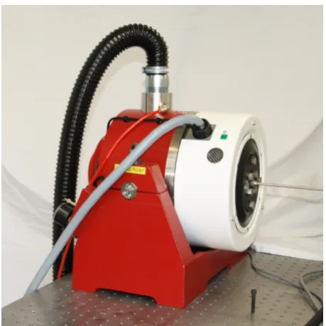
3.1.5 Laser Vibrometer . . . 42
3.1.6 Electrodynamic shaker and controller . . . 43
3.2 Specimens . . . 44
3.2.1 Aerospace panel . . . 44
3.2.2 Hastelloy plates for high temperature . . . 45
3.3 Method . . . 46
3.3.1 Digital Image Correlation . . . 46
Chapter 4 Assessment of Measurement Uncertainty . . . 51
4.1 Introduction . . . 51
4.2 RM Design and analytical description . . . 54
4.2.1 Design and manufacture . . . 54
4.2.2 Natural frequencies and deformation field equations . . . 55
4.3 Experimental procedure . . . 56
4.3.1 Apparatus . . . 56
4.3.2 Excitation and displacement measurement . . . 57
4.4 Results . . . 60
4.5 Discussion . . . 68
4.6 Conclusions . . . 71
Chapter 5 Application of PL-DIC for Vibration Measurement . . . 73
5.1 Introduction . . . 73
5.2 Image acquisition at resonance . . . 74
5.3 Image acquisition with random excitation . . . 76
5.4 Comparison to High-Speed DIC . . . 80
5.5 Results and discussion . . . 81
5.6 Conclusions . . . 88
Chapter 6 Validation of an Aerospace Component Simulation. . . 91
6.1 Introduction . . . 91
6.2 Experimental setup . . . 92
6.2.1 Dynamic calibration . . . 96
6.3 Simulation setup and results . . . 97
6.3.1 Simulation conditions . . . 100
6.4 Tchebichef decomposition . . . 102
6.5 Concordance . . . 110
6.6 Discussion . . . 114
6.7 Conclusions . . . 121
Chapter 7 High Temperature Vibration Measurements . . . 123
7.1 Introduction . . . 123
7.2 High temperature DIC . . . 124
7.3 Experiment . . . 127
7.3.1 Induction heating setup . . . 128
7.3.2 Quartz lamp setup . . . 131
7.3.3 Specimen preparation . . . 135
7.4 Simulation . . . 137
7.5 Results and discussion . . . 140
7.5.1 Induction heating . . . 140
7.5.2 Quartz lamp heating . . . 142
7.6 Conclusions . . . 149
Chapter 8 Summary . . . 151
Chapter 9 Conclusions . . . 157
Appendix A Airbus Panel Drawing . . . 161
Appendix B Airbus Panel Mode Shapes . . . 163
Appendix C Hastelloy Plate Mode Shapes . . . 167
Appendix D PL-DIC Random Capture . . . 171
References . . . 177
LIST OF TABLES
Table 2.1 Comparison of the different methods of image acquisition for fast-moving objects. In the case of the high-speed cameras, the expo-sure time refers to the minimum length of the expoexpo-sure (or shutter time) that can typically be obtained. In the case of the illumina-tion sources, it refers to the minimum time duraillumina-tion of each light pulse. . . 21
Table 3.1 Specifications of the shaker system. . . 43
Table 4.1 The critical dimensions of the cantilever Reference Material and their associated uncertainties. . . 55
Table 4.2 The fit parameters α and β along with their uncertainty values calculated from the field of deviations for each load step. . . 69
Table 4.3 Summary of the calibration uncertainty results for each of the three frequencies. N is the total number of experimental data points produced. u(dk) is the uncertainty from the residuals.
u(wk) is the uncertainty from the cantilever reference material.
ucal(wk) is the combined uncertainty, and the last column on the right is the percent uncertainty relative to the amplitude of dis-placement for that frequency. . . 69
Table 5.1 Comparison of digital image correlation systems based on high speed cameras and the system with standard cameras and the pulsed laser. . . 74
Table 5.2 Summary of the calibration uncertainty results for each of the three frequencies. N is the total number of experimental data points produced. u(dk) is the uncertainty from the residuals.
u(wk) is the uncertainty from the cantilever reference material.
ucal(wk) is the combined uncertainty, and the last column on the right is the percent uncertainty relative to the amplitude of dis-placement for that frequency. . . 80
LIST OF FIGURES
Figure 2.1 Flowchart for verification and validation activities for simulation and experimental methods [1]. . . 26
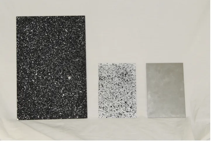
Figure 3.1 One of the large plates sprayed with a base coat of black paint and white speckle. The small plate in the middle has a base coat of white with a black speckle. The small plate on the right is un-painted. . . 45
Figure 3.2 An example of how DIC calculates displacements by tracking the deformation of a subset of the pixels in an image. . . 49
Figure 4.1 Drawing of the cantilever Reference Material showing the normal-ized dimensions of the specimen used as well as the gauge area that was imaged with the DIC system. . . 54
Figure 4.2 The experimental setup using the non-contacting loudspeaker for excitation (A). The image on the left gives an overall view of the setup showing the cameras (B), laser vibrometer (C) and light source (D). The image on the right is a close-up of the cantilever mounted in the vice. . . 58
Figure 4.3 Close up showing the 160mm x 40mm area of the cantilever Ref-erence Material mounted to the shaker. This excitation method was used for the second and third modes. . . 59
Figure 4.4 The predicted out-of-plane displacement from theory, wT(xi, yj),
(mesh surface) and the measured values from experiment,wE(xi, yj),
(solid surface) for the 1st mode of the cantilever at the two ex-trema of deflection. . . 63
Figure 4.5 The solid surface is the field of deviations, d(i, j), and the mesh surface is given byα+βwT for the measurement shown in figure 4.4. . . 63
Figure 4.7 The solid surface is the field of deviations, d(i, j), and the mesh surface is given byα+βwT for the measurement shown in figure 4.6 . . . 64 Figure 4.8 The predicted out-of-plane displacement from theory, wT(xi, yj),
(mesh surface) and the measured values from experiment,wE(xi, yj),
(solid surface) for the 3rd mode of the cantilever at the two ex-trema of deflection. . . 65 Figure 4.9 The solid surface is the field of deviations, d(i, j), and the mesh
surface is given byα+βwT for the measurement shown in figure 4.8. . . 65 Figure 4.10 The assessment plots produced based on the measurement shown
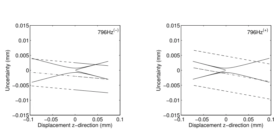
in figure 4.4. The solid line represents the uncertainty in the modal shape, ±2u(w), and the dashed line represents the uncertainty in the field of deviations, (α+βwT)±2u(d). . . 67 Figure 4.11 The assessment plots produced based on the measurement shown
in figure 4.6. The solid line represents the uncertainty in the modal shape, ±2u(w), and the dashed line represents the uncertainty in the field of deviations, (α+βwT)±2u(d). . . 67 Figure 4.12 The assessment plots produced based on the measurement shown
in figure 4.8. The solid line represents the uncertainty in the modal shape, ±2u(w), and the dashed line represents the uncertainty in the field of deviations, (α+βwT)±2u(d). . . 68 Figure 5.1 An image captured with a pulse from the laser illuminating the
vibrating component. Note the lens and diffusers used to obtain uniform illumination from the laser. . . 75 Figure 5.2 The phase stepping of the PL-DIC system. In this example the
images are being captured at 18 degree phase increments relative to the excitation signal. . . 76 Figure 5.3 The original experimental setup used for resonant excitation(top)
and the modified setup with the addition of the laser vibrometer used for random excitation(bottom). . . 78 Figure 5.4 An example of the velocity signal measured with the laser
Figure 5.6 The out-of-plane (z-displacement) at resonance of the flat panel measured using single frequency excitation and phase shifting of the image acquisition. . . 83
Figure 5.7 The FFT of the time history of the velocity signal from the laser vibrometer of the panel. . . 84
Figure 5.8 Four examples of different z-displacement measurements captured using the custom LabVIEW system and random excitation of the panel. . . 85
Figure 5.9 The FFT calculated from the laser vibrometer measurement that corresponds to figure 5.8. . . 86
Figure 5.10 The in-plane displacements and strains calculated from the top-left example shown in figure 5.8. . . 87
Figure 6.1 Picture of front of the experimental setup showing the cameras, laser vibrometer, and pulsed laser (left) and the back side of the panel showing the attachment to the shaker (right). . . 93
Figure 6.2 Front view of the panel showing the stinger attachment and the comparison area for the image decomposition. . . 93
Figure 6.3 Diagram showing the arrangement of the experimental apparatus and the attachment of the shaker. . . 95
Figure 6.4 Images captured by the PL-DIC system of the cantilever at six different positions in the field of view. Locations 1-3 are with the cantilever horizontal and 4-6 are vertical. . . 97
Figure 6.5 Close-up of the 3-D meshes used for the FE simulations. The man-ually meshed model (left) consisted of 170k brick elements. The computer-generated tetrahedral mesh(right)consisted of 115k el-ements. . . 99
Figure 6.6 The z-component of displacement plotted on the deformed shape from the eigenvalue analysis for the first three modes of vibration. 99
Figure 6.7 The out-of-plane displacement measured in the experiment (left) compared to the results from the FE modal frequency analysis (right). . . 101
Figure 6.9 An example of the feature vector produced from the Tchebichef decomposition. In this case it can be seen that the first and third moments are significantly larger than the others. . . 104 Figure 6.10 Plot ofSM againstSE for the baseline (a), constant damping (b),
string constrained (c) and tetra-meshed (d) simulations of the first mode. . . 107 Figure 6.11 Plot ofSM againstSE for the baseline (a), constant damping (b),
string constrained (c) and tetra-meshed (d) simulations for the second mode. . . 108 Figure 6.12 Plot ofSM againstSE for the baseline (a), the constant damping
(b), the string constraints (c) and the tetra-meshed (c) simulations for the third mode. . . 109 Figure 6.13 Comparison of the different cases the concordance correlation
co-efficient takes into account. . . 111 Figure 6.14 The concordance, accuracy, precision, and scale shift plots for the
first mode of vibration corresponding to the results from figure 6.10.113 Figure 6.15 The concordance, accuracy, precision, and scale shift plots for the
second mode of vibration corresponding to the results from figure 6.11. . . 114 Figure 6.16 The concordance, accuracy, precision, and scale shift plots for the
third mode of vibration corresponding to the results from figure 6.12. . . 115 Figure 7.1 The amount of black body radiation of an object as a function of
temperature and wavelength. . . 125 Figure 7.2 Comparison of the quantum efficiency of the CCD camera used in
the induction heating experiments and the transmission efficiency of the blue bandpass filter. . . 126 Figure 7.3 The original coil (CL-1) that created hot spots at the top and
bottom edges of the plate (top left). This coil was reshaped to make it more rectangular and redesignated MOD-1 (top right). A smaller circular coil (CL-2) that did not overhang the edges (bot-tom left). The final iteration that gave the best results, designated RT-1 (bottom right). . . 129 Figure 7.4 The front side of the specimen with the thermocouple wires
Figure 7.5 Plot of the measured temperatures against the setpoint temperature.132 Figure 7.6 Picture of the quartz lamp heating setup with the large plate
mounted to the shaker. . . 133 Figure 7.7 Scale drawing of the quartz lamp heating setup showing the
ar-rangement of the different devices that were used in the experiments.134 Figure 7.8 The effect of using the pulsed laser and filter on the images.
Pic-ture without the pulsed laser (a) and with the pulsed laser and bandpass filters (b). . . 135 Figure 7.9 The temperature of the large plate in various heating configurations.136 Figure 7.10 One of the small plate samples prepared by dabbing the speckle on
with a sponge (left). The back of the plate showing the oxidation due to heating(right). Note the discolouration at the edges of the plate caused by uneven heating. . . 137 Figure 7.11 The first four real eigenmodes of the small Hastelloy plate. . . . 138 Figure 7.12 The first four real eigenmodes of the large Hastelloy plate. . . 139 Figure 7.13 Comparison of the temperature distribution calculated from xx
(a) and the Matlab generated FE mesh with the temperature-dependent modulus values (in GPa) overlaid (b). . . 139 Figure 7.14 Images captured using a blue bandpass filter and blue LED
light-ing. Images were captured incrementally from 100 ◦C to 600 ◦C in 100 degree increments. It is possible to see the slight discol-oration of the paint and the glowing at the top and bottom edges in the 600 ◦C image. An alternative colormap is used to increase contrast for the reader. . . 141 Figure 7.15 Comparison of the experimentally obtained mode shapes for the
120x80mm plate with induction heating and the predicted results from the simulation. . . 143 Figure 7.16 Comparison of the frequency response function for the 219x146mm
plate at room temperature and elevated temperature. . . 145 Figure 7.17 The full-field temperature map generated by the thermal camera.
Figure 7.18 Comparison of the contour of the unheated and heated plates. The heating direction indicates the face of the plate that was oriented towards the quartz lamps. . . 148 Figure A.1 Drawing of the airbus panel . . . 162 Figure B.1 Real eigenmodes 1-10 of the aerospace component simulation. . . 164 Figure B.2 Real eigenmodes 11-18 of the aerospace component simulation. . 165 Figure C.1 The first 10 real eigenmodes of the small (120x80 mm) Hastelloy-X
plate from simulation. . . 168 Figure C.2 The first 10 real eigenmodes of the large (219x146 mm)
Hastelloy-X plate from simulation. . . 169 Figure D.1 The full set of the first series of out-of-plane displacement captured
using PL-DIC with random excitation. . . 172 Figure D.2 The full set of the second series of out-of-plane displacement
cap-tured using PL-DIC with random excitation. . . 173 Figure D.3 The full set of the third series of out-of-plane displacement
Chapter 1
Introduction
1.1
Motivation
One of the most common failure modes in aircraft structures is material and structural fatigue. Despite a considerable improvement over the last several decades, the reliable prediction of fatigue life continues to be a challenge, especially for complex structures operating in extreme conditions such as those encountered during hypersonic flight. This combined high-temperature and vibration environment is not well understood. There is a considerable cost and complexity associated with performing experiments under these conditions, and so simulation is heavily relied upon. Better simulations are needed to meet strict weight and performance requirements, and to make them better they need to be validated with high-quality experimental data. Full-field optical measurement techniques such as Thermoelastic Stress Analysis (TSA) or Digital Image Correlation (DIC) are capable of producing maps of stress and strain which can be used for validation purposes. However, these techniques need further development to be suitable for use in a combined thermal and vibration environment.
testing specimens up to 300x450 mm in size with sound pressure levels of 180 dB and temperatures up to 1370 ◦C. The heating is provided by quartz lamps, which produce a heat flux of around 1125 kW/m2. The second chamber is much larger and designated the Combined Environment Acoustic Chamber (CEAC). It is capable of testing specimens on the order of 2 meters square, at similar sound pressure levels and temperatures as the SEF. Currently in these facilities they are only able to make certain measurements during an experiment, usually limited to some strain gauge or other pointwise techniques on the back surface of the panel. Ideally, they desire to make full-field measurements on the front, heated side of the panel, with the aim of using the data for the validation of computational mechanics models.
1.2
Background
A large amount of the research in the area of thermoacoustic fatigue has been driven by the quest for hypersonic flight. The very high speeds encountered during sustained hypersonic flight generate aerothermal and aeroacoustic loading of the exterior of the vehicle. In addition, the engine generates heat and acoustic loading on parts of the structure. This creates a situation in which components can fail from either the acoustic and vibration loads, thermal cycle and mechanical loads, or excessive temperature [3].
CHAPTER 1. INTRODUCTION cancelled [4]. Therefore, there is a strong motivation to develop techniques that permit validation-quality data to be acquired in efficient and realistic experiments that address both the structural and temperature aspects.
The majority of structural level testing in this area has been performed using a pro-gressive wave tube (PWT). A PWT is capable of simulating wideband random excitation up to sound pressure levels on the order of 160 dB and are typically sized to test compo-nents that are 1 meter by 0.5 meter [5]. Steinwolfet al. showed that with modern digital feedback control, it is possible to tailor the acoustic output of a PWT to closely match that of a jet engine [6].
Recently, an experiment was conducted using the AFRL SSC and the Propulsion Directorate’s large scale supersonic combustion research facility by Beberniss et al. [4]. A high-speed continuous flow wind tunnel (designated RC-19) was used to subject a small, thin steel panel to a shock impingement. The response of the panel was measured using 3D digital image correlation with a pair of high speed cameras to get displacement and strain information.
All of the tests performed in a PWT so far have utilized point-wise measurement methods such as strain gauges and laser vibrometers. The test by Beberniss et al. using the high speed wind tunnel is one of the few examples of digital image correlation to measure the vibration response of a panel. For the purposes of validation of computational models for life prediction of a component, single measurements may not be sufficient. There is a need for high quality, full-field data from structural vibration experiments.
uncertainty in experimental measurements made using full-field methods. All of these things will need to be considered in the development of a validation procedure that uses full-field experimental data.
The use of digital image correlation for high temperature measurements is relatively recent, and the process is still maturing. Most of the published results are 2-D ments of static or quasi-static experiments. It is only recently that dynamic measure-ments have been attempted at high temperature. Abotula et al. used a pair of high speed cameras to capture the deformation of Hastelloy samples at various temperatures under shock wave loading [7]. As the ultimate goal is to use the validation procedure on thermoacoustic computational models, there is a need to develop the DIC technique to be suitable for use in a combined high temperature and vibration environment. It is not until this has been addressed that validation can be attempted.
1.3
Aims and objectives
The long-term aim of this project is to develop and implement a methodology to measure strain and stress fields in structural aerospace components at AFRL during thermoacous-tic fatigue loading for the purposes of model validation. The research presented here was funded by the U.S. Air Force to take the first steps towards that ultimate goal. The specific objectives of this thesis are therefore to:
• develop a low-cost methodology to measure validation quality data during vibration loading.
• perform a validation of a computational solid mechanics model using full-field ex-perimental data from an experiment with dynamic loading.
Chapter 2
Literature Review
The desire to achieve hypersonic flight, or flight at speeds in excess of Mach 5, has pre-sented many challenges to the materials and structural design community. One such challenge is thermoacoustic fatigue resulting from the hypersonic flow and acoustic pres-sure from the engine. There have been several major phases of research on thermoacoustic fatigue in relation to experimental project planes sponsored by the U.S. government. The first such program was for the X-15 plane, which lasted from 1954 to 1968. The X-15 vehi-cle was rocket-powered, which meant that it did not require oxygen from the atmosphere to produce thrust.
The next major hypersonic program was the X-30 National Aerospace Plane (NASP), which started around 1982 and lasted just over a decade until it was cancelled in 1993. The X-30 was a joint program between NASA, DARPA, and the USAF to create a hypersonic, single-stage to orbit vehicle. Unlike the X-15 program, the X-30 was intended to be powered by an air-breathing scramjet engine. This type of engine configuration presented some unique challenges in terms of high temperature acoustic loading on the inlet ramp and exhaust portions of the engine.
encounter extreme conditions [8], including:
• Extremely hot surface temperatures
• Large temperature gradients
• Transient heating
• Very high acoustic pressures
The potential implications of these extreme conditions were extensive:
• Large static (thermal) stresses superimposed on dynamic stresses
• Changes in material properties that manifest as changes in strength and modulus of elasticity
• Accentuation of non-linear behavior
• Changes in fatigue behavior
• Complex thermal and structural boundary conditions that may be difficult to sim-ulate experimentally
• Difficulty obtaining reliable experimental structural response measurements
CHAPTER 2. LITERATURE REVIEW
Research into scramjet engines currently continues in the X-51 Waverider program which was initiated in 2004 by the U.S. Air Force. Like the X-43 vehicles, the X-51’s are not designed to be recovered after flight. A total of four vehicles have been built, with one successful test flight so far, which occurred in 2010. The vehicle was launched from a B-52 and under rocket power attained a speed of Mach 4.5, at which point it transitioned to scramjet power for 200 seconds, reaching Mach 5.
While there has undoubtedly been a wealth of experimental data collected from the flights of the X-43 and X-51 programs, it does not appear to have been publicly released at this point. Research in the acoustic and thermoacoustic area has continued in the public domain, but it has been more focused on modeling and simulation, with a few exceptions.
As the aim of this thesis is to increase the understanding of the coupled thermoacous-tic fatigue failure of aircraft structures and materials through the development of novel, full-field experimental methods, this review will focus on the experimental aspect of the research in this area. Experimental and numerical methods have developed in tandem over the last several decades of research into thermoacoustic fatigue, but the experimental methods have been lagging behind until recently when there has been more widespread use of optical techniques, high speed imaging systems, and increased computational ca-pabilities.
the X-43 program as well as other funding initiatives such as the US Air Force Structural Sciences Center.
The second part discusses different methods of acquiring full-field displacement and strain data with the aim applying the techniques to a vibrating component. This includes methods that cover a wide range of physical scales and types of data capture.
The third part gives a review of the recent developments in validation methodologies for full-field measurement techniques. Although the use of experimental data for the validation of computational models certainly is not a new topic, the use of full-field methods is relatively recent. This is due largely to the complexity of making a meaningful comparison with large amounts of data. An important aspect of validation is uncertainty quantification, so this part includes a section to review that.
The final part examines the state of the art in high temperature DIC and TSA ex-periments. Particular interest is the use of these techniques with vibration or other experiments that require high speed imaging.
2.1
Vibratory panel experiments
CHAPTER 2. LITERATURE REVIEW
spectrum broadened and the frequency peak shifted down. Some limited results for stress level as a function of the number of cycle were given for two of the panels. The analysis was focused only on the acoustic aspects and did not include any information on thermal effects.
Work was done by Schneider at the Lockheed-Georgia Company under Air Force funding to establish tolerance levels and design criteria for acoustic fatigue prevention in flight vehicles [10]. Experiments were performed on 7075-T6 aluminum and 6Al-4V titanium specimens at room temperature and at elevated temperature. The elevated temperature for the aluminum specimens was 150 ◦C and the elevated temperature for the titanium specimens was 315 ◦C. This was primarily an experimental program, but some initial analysis was performed to establish the parameters to be measured and also to correlate with the experimental results. The first set of experiments were of cantilever beam specimens approximately 50x150 mm. The specimens were clamped at one end and excited using random amplitude vibration on a shaker. Strain gauges were placed at the root of the cantilever near where the parts were clamped, but gauges were only used on the room temperature specimens. Periodic inspections using sine wave excitation were performed to determine the natural frequency of the specimen as the test progressed. The specimens were considered to have failed when the resonant frequency had decreased by 2%.
response frequency. If the panel had a single-mode response, a narrow 100 Hz bandwidth excitation spectrum was used. If the panel had a multi-mode response, a bandwidth of approximately 300 Hz was used, which was shaped to obtain a flat response using 1/3 octave band spectrum shaper. The panels were inspected periodically during testing, at intervals ranging from 15 minutes to an hour, based on the amount of time that had elapsed since the start of the test. For the elevated temperature tests, this meant that the panel had to undergo a cooling and re-heating cycle every time it was inspected.
The gauges also had limited fatigue life due to the large amplitudes encountered during testing. The study produced a large amount of experimental data, however Schneider found that for the more complicated stiffened panels, the results didn’t correlate very well with the analytical models. Particularly for the thermal buckling, as it was assumed in the analysis that the substructure was thermally isolated.
Leatherwood et al performed a series of tests on simulated aircraft panels made from carbon-carbon composite and also a system being developed which was called the Thermal Protection System [8]. The tests were performed using the Thermal Acoustic Fatigue Apparatus (TAFA) at the NASA Langley Research Center. The TAFA is a progressive wave tube type testing facility that provides acoustic energy using a pair of WAS 3000 electropneumatic modulators with 30 kW of power each. These modulators can produce an OASPL of 135-169 dB over a spectrum of 30-500 Hz. The facility can test a panel up to 1.5 m square, and can provide heating using a bank of 12 quartz lamps. The lamps produce 2500 W of power each, resulting in approximately 45.4 kW/m2 of heat flux.
CHAPTER 2. LITERATURE REVIEW
with sodium silicate. This made the installation of strain gauges onto the surface a very difficult process, requiring microblasting, baking, application of ceramic adhesives, curing, and plasma spray application of various coatings. The flat panels were installed into the chamber fully clamped around all four edges in a picture frame type of fixture. The blade-stiffened panels were only clamped on the two sides parallel to the stiffeners while the other two sides were left free.
Unlike the carbon-carbon panels, the TPS panels were not tested to failure. The composition of the panel consisted of a superalloy honeycomb made of Inconel, titanium, Dynaflex, and Q-fiber. Three different panels were tested, with three different skin thick-nesses. The total panel thicknesses were approximately 60 mm. As the TPS panels had a metallic skin, traditional high temperature strain gauge adhesives and application meth-ods could be used. The maximum measured strain was on the panel with the thinnest (64 micron) skin, which was 33 microstrain at 160 dB.
to the boundary conditions imposed on them. As they were only clamped parallel to the stiffeners, it was conjectured that the stiffeners provided no benefit but rather added mass which contributed to the failure occurring sooner. Both the flat and the blade-stiffened panels did show increased fatigue performance at the elevated temperature test, which was encouraging.
The carbon-carbon panels had a high rate of gauge failure as compared to the TPS panels. Low indicated strains of only 5-20 microstrain were thought to be erroneous, but later analysis revealed that it might have been due to non-linear stiffening in the panels.
An extensive report was released by Blevins et al. which was the second phase of a three phase study sponsored by AFRL [11]. The aim of the study was to identify a typical trajectory into orbit and to use that to determine the aerothermal and acoustic loads that a vehicle would encounter. These loads were used to design forebody, ramp, stabilizer, and nozzle skin panels which were then analyzed to determine the temperatures as well as the mean and dynamic stresses in the panels. The report includes results from extensive analysis of the panels, but it was planned to do the testing and validation in the third phase, for which there was a detailed validation and verification plan. If the third phase of research has been completed, it does not appear to have been released publicly at this point.
CHAPTER 2. LITERATURE REVIEW
main candidate materials were considered: carbon-carbon panels with a silicon-carbide coating, and titanium metal matrix composites (TMC). The blended wing body (BWB) concept that was analyzed has the engine placed amidships such that the forebody acts as a compression surface for the engine, and the aftbody acts as an expansion nozzle. As a consequence, the forebody, ramp, and nozzle panels are subjected to severe thermal and acoustic loading. Blevinset alestimated for the projected 100 flight life cycle for the BWB concept that these panels would encounter over 20 million vibration cycles.
Designs were proposed for the forebody and ramp panels that were carbon-carbon construction with blade stiffeners. The designs for the two panels were similar, but the ramp panel was not required to bear any structural loads, so it had a wider stiffener spacing and a thinner skin. It was determined that the peak heat flux in the panels could be as high as 600 kW/m2 with temperatures ranging from 1140-1790 ◦C, depending on ascent trajectory and the laminar/turbulent flow. The aeroacoustic loading on the panels was found to be 130-145 dB, while emissions from the engine could be as high as 170 dB. The analysis showed that the lowest mode of vibration for the forebody panel was 524 Hz, and the lowest mode for the ramp panel was 258 Hz.
stiffening, the loads exceeded the fatigue capability of the panel.
Also as a result of the NASP, a large scale supersonic combustion research facility was created at Wright-Patterson AFB [12]. The combustion facility was designated as RC-19 and contains a primary test section that is 150 mm wide and 130 mm high, and contains viewing windows made from fused silica. While primarily designed to study combustion in flows up to Mach 2, Beberniss et al recently used the RC-19 facility along with high-speed 3D digital image correlation to capture the dynamic response of a panel subjected to shock impingement [4].
During this same time period there was some research into acoustic fatigue conducted at the Institute of Sound and Vibration Research at the University of Southampton. The research was primarily motivated by the commercial aircraft industry, and therefore only included temperatures which were moderately elevated above ambient. White performed analysis and experiments using carbon fiber specimens at room temperature and at 120◦C [13]. PWT testing was conducted on specimens made of XAS/914 carbon fiber that were 450 mm by 300 mm and 1.75 mm thick. It was noted that the response of panels tested in a PWT can vary from actual conditions because of a higher damping in the panel caused by acoustic interaction with the tunnel.
White had previously noted that for very thin (metallic) plates excited by high sound pressure levels the response was nonlinear [14]. Ng and White also found that if there was compressive in-plane loading, there were nonlinear effects immediately before buckling and post buckling, as well as modal coupling [15]. Ng then examined the snap through effects in the post-buckled regime [16].
CHAPTER 2. LITERATURE REVIEW
[18]. The panels were 912 mm by 525 mm and mounted into the PWT using four circular steel springs. Initial experiments were performed using a glass/fiber epoxy picture frame type clamping arrangement, but it induced extra stiffness in the panels and lowered the strain response. Using the steel springs, the measured natural frequencies were close to those calculated for the free response in Ansys. The panels were excited using broadband noise in the 60-600 Hz range at an overall sound pressure level of 164 dB. The maximum RMS strain recorded were on the order of 250 microstrain.
One of the few papers which discuss the use of full-field methods to measure a vibrating panel was performed by Beberniss et al. at the Air Force Research Laboratory [4]. They used stereoscopic digital image correlation to measure a 305 mm by 152 mm by 0.635 mm thick 4130 steel panel mounted in the RC-19 large scale combustion research apparatus. The design of the tunnel necessitated that the panel be viewed through a window, which consisted of a 19 mm thick quartz panel. The panel was clamped in a picture-frame fashion, and was subjected to a shock impingement with a nearly Mach 2 flow. Measurements were made using a pair of high speed cameras with 32GB of memory each and 5000 frames per second with a 640x352 pixel array size.
that the resulting PSD was fairly noisy. The results for 10,000 frames were slightly better, and those from the entire 100,000 frame recording were the best. There was found to be good agreement between the DIC measurements and those made with the laser vibrometer and the strain gauge. In an effort to reduce processing time, the DIC measurements were calculated at 21 discrete points on the panel rather than computing the entire displacement field.
2.1.1
Conclusions
There has been a fair amount of panel testing with broadband excitation over the last 50-60 years. There are really only a few facilities available in which to perform such exper-iments, as a large acoustic test chamber capable of 160+ dB sound levels is undoubtedly expensive. Most of the data was collected using traditional measurement techniques such as strain gauges or accelerometers. The one exception is Beberniss et al, who used high speed DIC to measure the response of a steel plate to a Mach 2 airflow [4]. Unfortunately, due to the issues of processing the 200,000+ images resulting from the test, they did not calculate the full-field response of the panel but rather looked at 21 discrete points.
Most of the results were also captured at room temperature or with moderate heating. Schneider did use some quartz heating of the specimens, but only to a few hundred degrees (◦C). The measured strains are not very high with this type of excitation, usually only a few hundred microstrain. Leatherwoodet al. did obtain temperatures up to 650◦C in there experiments, but had several challenges involving the failure of the heating lamps and of the strain gauges. They also observed non-linear behavior due to the high acoustic loading used in their experiments [8].
CHAPTER 2. LITERATURE REVIEW
subjected to various loading conditions. However, these analyses are not valid for the non-linear behavior of plates, which tends to occur when there is very high loading [16], or combined effects [15].
2.2
Full-field experimental methods
There are many different optical techniques available that permit the measurement of various components of displacement and strain. Generally speaking, there are two main types: Interference methods which use coherent light and methods that use non-coherent light. Interference methods include such techniques as photoelasticity and holography and rely on the wave properties of light. Non-coherent light techniques include fringe projec-tion, grid methods, and digital image correlation. Each method has its own advantages and disadvantages, and some are better suited to dynamic and high-speed measurements than others.
2.2.1
Interference methods
deformation.
In speckle interferometry slightly different arrangements are used to measure in-plane and out-of-plane displacements [20]. To measure out-of-plane displacements, a single beam is split into a reference beam which is directed to the image plane, and a beam which is directed to the surface of the object. To measure in-plane displacements, two separate beams are directed at the surface. This provides the displacement component of the surface in the plane of the beams. If the beams are rotated 90 degrees, then the second component of displacement can be measured. Special measurement systems have been created which combine these components to be able to simultaneously measure the in-plane and out-of-plane displacements.
In shearography, a device is placed in front of the image plane to shear the reflected beam from the surface of the object. Leendertz and Butters proposed a device which used a Michelson interferometer to shear the beam [21]. Hung et al. used a plate with four apertures which was moved relative to the image plane to produce the shearing effect [22]. This method effectively performs the first step of differentiation of the surface displacement, producing fringes that are related to the slope of the surface (for out-of-plane measurements) or the in-plane strains (for in-plane measurements). This is useful to find the strain at the surface of an object in a particular direction. Similar to interferometry, the system must be rotated by 90 degrees to obtain the full strain field.
2.2.2
Other methods
CHAPTER 2. LITERATURE REVIEW
surface of the object, permitting the measurement of the contour. However, the technique by itself is not suitable for measuring in-plane deformation.
The grid methods and DIC are somewhat similar in that they both operate on the intensities measured from the surface of an object that is covered with a pattern. In digital image correlation, a random pattern is necessary on the surface of the object. Sometimes, the natural texture is sufficient, but typically the best results are obtained by applying a high contrast, random speckle pattern to the surface. The grid method requires that a very precise, high resolution grid is created and then applied to the surface of the object [23]. In both methods the deformation of the pattern is tracked from one image to the next in order to create a map of displacements for the surface of the object. The displacement map can then be differentiated to obtain strains.
The advantage of using a grid over a random pattern is that a smaller subset of pixels is required to map the deformation from the reference image. For example, Pierron et al. used the grid method with a 6x6 pixel subset size for the measurement of strains in a composite open-hole specimen subjected to tensile loading [24]. A variation of the method was developed by Badulescu et al. to directly compute the strains from the intensity map without computing the displacements first [25]. This reduced the noise that is normally introduced in the differentiation process when computing strains from displacements. The technique has also been shown by Ri et al. to be able to measure relatively small displacements over a large field of view [26]. They obtained a noise level of less than 4 microns over a 1000 mm field of view. The primary disadvantage of the grid method (at this point) is that it is only suitable to measure in-plane displacements.
reflected light is then passed through a grid which produces a phase map relating to the slope contours of the object. The technique has the advantages of directly measuring the slope and is relatively insensitive to vibrations because it measures the direction of light propagation and not a path length difference like interference methods. More recent measurements have simplified the technique and demonstrated that it is not necessary to use coherent light [29].
2.2.3
Application to vibration measurement
Recent advances in computers and camera sensor technology means that most techniques can be performed digitally, without the use of photographic films or other mediums. There are two primary types of imaging sensor: the charge-coupled device (CCD) and the complimentary metal-oxide-semiconductor (CMOS). Laboratory and machine vision cameras tend to have CCD sensors while high-speed cameras have CMOS sensors. This means that for the capture of vibration or other dynamic events, the limitation is usually in the imaging system. The interference methods are an exception, as they often require phase-stepping, in which multiple images would be acquired at the same object state. However, for steady-state vibration measurements, the interference methods permit the use of time-averaging to capture modal information. To accomplish this the measurement duration is set to be longer than the period of vibration. This works because the vibrating object spends most of its time at the extrema of vibration, so this is what is recorded by the imaging system. Moreau et al. used time-averaged electronic speckle pattern interferometry to measure the vibration of a 100x150x5.1 mm PVC plate [30].
CHAPTER 2. LITERATURE REVIEW
to freeze the motion of an object such that it can be recorded by a camera. There are many different types of light source which have varying intensity and pulse duration. This type of illumination has been used successfully in many types of measurement in the past and has recently been applied to digital image correlation [31, 32, 33]. Table 2.1 gives an overview of the different acquisition and illumination methods.
Table 2.1: Comparison of the different methods of image acquisition for fast-moving objects. In the case of the high-speed cameras, the exposure time refers to the minimum length of the exposure (or shutter time) that can typically be obtained. In the case of the illumination sources, it refers to the minimum time duration of each light pulse.
Type Exposure Time Frequency
High-speed cameras Continuous, bright light 1µs 100,000+ Hz Stroboscopic illum. Arc lamp, LED, etc. 10 µs 10,000 Hz Pulsed-Laser illum. Nd:YAG laser 4∗10−3 µs 10-100 Hz
Patterson and Greene used stroboscopic illumination for the photoelastic analysis of compressor blades [34, 35]. The compressor blades were excited at a resonant frequency using a high speed air jet. Synchronization of the blade vibration and the stroboscopic illumination was performed by displaying signals from vibration and illumination sensors on an oscilloscope and adjusting the strobe pulse by use of a skew control. This allowed the point of maximum excursion of the blade to be captured by the camera sensor.
Hanet al used a pulse modulated laser diode to make photoelastic modulated (PEM) ellipsometry measurements of thin films [36]. The laser was sent through a photoelastic modulator and then a beam expander, before it was reflected off of the surface of a specimen and read by a CCD camera.
Moneron et al used a xenon arc lamp with a 10 microsecond flash duration and a repetition rate of 15Hz for optical coherence tomography [37]. For the procedure, two CCD cameras are used to capture interferometric images which could not have any motion blurring.
or even LEDs, it is also possible to get good results using pulsed laser illumination. This method has the advantage of having very short pulse duration as compared to more traditional methods, which allows the capture of very fast motion. To make measurements of a flywheel rotating at high speed, Schmidt et al. found that traditional arc-discharge light sources did not have a short enough pulse duration, so they used a pulsed laser with a single CCD camera [31]. They used a Nd:YAG laser with a 6 nanosecond pulse duration, which permitted measurements of the flywheel of speeds up to 35,000rpm.
There are even techniques which take advantage of the double-pulse capability of lasers to be able to capture two images separated by some fixed time. Pedrini et al. used double-pulse electronic speckle pattern interferometry to measure vibrating objects [38, 39]. The system they used was capable of firing the laser pulses with a delay of 5-1000 microseconds between them. Two different experimental arrangements were used; a single-beam system to measure out-of-plane displacement and a dual-beam system to measure in plane deformation in one plane. There have been commercial systems created that use three beams and three cameras to fully capture the deformation of the surface [40].
Another possible approach to capture images of a vibrating component is to use very bright, constant illumination and a short shutter time [41, 42]. With this method, the motion of the object is frozen by the very short shutter time. For example, the AVT Stingray firewire camera has a minimum acquisition time of 20 microseconds. Poncelet et al used this approach to make DIC measurements of a steel specimen during a biaxial fatigue test [41]. The illumination was provided by two 400W tungsten lights and two 3x3W LED arrays.
CHAPTER 2. LITERATURE REVIEW
typically have minimum acquisition times of 1 microsecond and framerates that can ap-proach 1 million frames per second. The trade off is that as the framerate is increased, resolution typically decreases. For a high speed camera to achieve its maximum fram-erate, the image array size may only be 64x12 pixels. This is a disadvantage for digital image correlation, as it will cause a decrease in the spatial resolution [43].
Reu published a survey of high and ultra-high speed cameras along with some prac-tical considerations for DIC measurements [44]. To achieve their extreme framerates, ultra-high speed cameras employ various methods including rotating mirrors, beam-split optical paths, and memory on the chip. These cameras all have issues with DIC that have to be addressed to make quality measurements. High-speed cameras, on the other hand, are somewhat better suited to DIC measurements. The cameras typically use a large complementary metal-oxide-semiconductor (CMOS) sensor as opposed to the CCD more commonly used in machine vision cameras. One potential issue with both types of cameras is synchronization. If the cameras are not properly synchronized, large errors in the measurements could result.
2.2.4
Conclusions
Interferemetric methods like speckle interferometry and shearography are capable of pro-ducing accurate measurements with high resolution, but they tend to be sensitive to vibrations in the environment. Speckle interferometry is particularly susceptible to vi-bration, typically confining it to use on an optical bench. Shearography is more vibration resistant, but it still requires a somewhat complicated setup which might limit its use in an environment such as the CEAC.
relatively simple, requiring only two cameras to capture both in-plane and out-of-plane deformations. The sensitivity of the technique is largely dependent on the quality and array size of the camera sensor, and so as improvements are made DIC will benefit directly. DIC is perhaps not as sensitive as the grid methods, but it is capable of measuring object contour and out-of-plane deformation. It also may be more adaptable to high temperature measurements, as there are commercially available high-temperature paints. Deflectometry appears promising for the direct measurement of strains in vibrating plates, but requires the application of a reflective coating that might not work well at high temperatures.
In order to capture transient events, high speed cameras are really the only option. However, for single frequency excitation there are other methods that are less expensive and can provide better results. With pulsed illumination, it is possible to use standard cameras that are much smaller and capable of recording at higher resolutions than their high speed counterparts. In addition, specialized sensors that are sensitive to other parts of the electromagnetic spectrum outside the visible range (UV and IR) are not available in high speed cameras.
2.3
Validation
CHAPTER 2. LITERATURE REVIEW
which defined minimal requirements for a numerical study for a paper to be considered for publication.
The most recent document published concerning the solid mechanics community is the 2006 ASME Guide for Verification and Validation in Computational Solid Mechanics (ASME V&V) [1], which incorporates material from a paper published a few years earlier by Oberkampf et al. [47]. An overview and summary of the guide was published by Schwer [48], who was the chair of the Performance and Test Codes (PTC) 60 committee that produced the guide. In the overview, Schwer states that one of the most common misconceptions about the ASME V&V guide was that it would provide a definitive ver-ification and validation procedure for computational solid mechanics. Rather, it is a “foundational document” which provides a framework and defines terminology to create a standardized language. The flowchart in Figure 2.1 outlines the procedure that should be followed to compare simulation outcomes and experimental outcomes. The relevant terms defined in the ASME guide are included throughout this section, and are given in bold type.
The guide is broken up into four main sections: Introduction, Model development, Verification, and Validation. The primary concern of this thesis is the validation section, which deals with the comparison of the computational model and experimental results. Often, the terms verification and validation are used interchangeably, but there is a distinction between them:
verification: the process of determining that a computational model accurately represents the underlying mathematical model and its solution;
validation: the process of determining the degree to which a model is an accurate repre-sentation of the real world from the perspective of the intended uses of the model.
Reality of Interest
(Component , Subassembly, Assembly, or System)
Conceptual Model Abstraction
Mathematical
Model Physical Model
Computational Model
Experiment Design
Simulation Results Experimental Data
Simulation Outcomes Experimental Outcomes Quantitative Comparison Acceptable Agreement ?
Next Reality of Interest in the Hierarchy Physical Modeling Mathematical Modeling Implementation Calculation Uncertainty Quantification Implementation Experimentation Uncertainty Quantification Preliminary Calculations Yes No Revise Appropriate Model Or Experiment Validation Code Verification Calculation Verification
[image:44.595.97.540.130.684.2]Modeling, Simulation & Experimental Activities Assessment Activities
CHAPTER 2. LITERATURE REVIEW
algorithms used by the software are correct and that they produce accurate results, while the validation process ensures that physics of the model are correct by comparing the results to experimental data. There are also several different types of models, each representing a different concept or component.
model: the conceptual, mathematical, and numerical representations of the physical phe-nomena needed to represent specific real-world conditions and scenarios. Thus, the model includes the geometrical representation, governing equations, boundary and initial conditions, loadings, constitutive models and related material parameters, spatial and temporal approximations, and numerical solution algorithms.
Both the ASME guide [1] and Oberkampf et al. [47] discuss the use of metrics to make a quantitative comparison between the simulation outcomes and the experimental outcomes. The two sources differ slightly in the wording of the definition of “metric,” but it is essentially a measure. The metric should quantify both errors and uncertainties, and “actively resolve assessment of confidence for relevant system response measures for the intended application of the code” [47]. In essence, the ideal metric would provide a num-ber indicating the level of confidence in the agreement between the simulation outcomes and experimental outcomes, taking into account the error and respective uncertainties.
according to the following equation [51]:
RelativeError = computation−measured
measured (2.1)
The relative error metric can be effectively applied to point comparisons or lines of data, but is not very effective for more complex comparisons. For example, it is not a good choice to compare tensors, or data with time or spatial components. Also, as the measured value approaches zero, the quantity becomes undefined. This can be a problem for comparing things like waveforms, in which the signal can cross zero.
Full-field data presents similar challenges, and so the comparison is still often reduced to checking a few points rather than using the full data set. There are studies available which describe the collection of data using full-field methods, but do not explicitly de-scribe the validation procedure, e.g. [34]. This gap was recently addressed by the author and his coauthors who proposed a quantitative procedure for validating computational solid mechanics models based on full-field measurements of strain and or displacement plus the measurement uncertainty [52].
CHAPTER 2. LITERATURE REVIEW
moments are better suited to detecting global features, while Krawtchouk moments are suited to detecting local features [57].
Wang et al. have used a variety of shape descriptors to tackle full-field data from various engineering problems. They used a modified Zernike descriptor to compare the strain around a hole of a plate loaded in tension to the results from a computational model [58]. They have applied the Tchebichef moments to examine mode shapes resulting from vibration measurements [59], and an adaptive geometric moment descriptor for the vibration of a car bonnet liner [60]. The adaptive geometric moment descriptor was also used to track the evolution of damage to the car bonnet liner subjected to an impact from a high speed projectile [61]. Sebastianet al. used Tchebichef descriptors to compare strain data from a composite protective panel to simulation under compressive loading [62]. Recently, Allemang et al. used Principal Component Analysis to compare two sets of experimental data from frequency testing of an automobile chassis [63].
2.3.1
Measurement Uncertainty
According to the International Vocabulary of Metrology (VIM) published by the BIPM, uncertainty 1 can be evaluated by two methods [64]:
Type A: evaluation of a component of measurement uncertainty by a statistical analysis of a series of observations;
Tybe B: method of evaluation of uncertainty by means other than the statistical analysis of a series of observations.
are provided, including evaluation based on information: associated with authoritative published quantity values, obtained from a calibration certificate, and drift, (among oth-ers).
The majority of the literature deals with statistical analysis of measurement results, so Type A. There are many different components that contribute to the measurement uncertainty, and it is understood that it is not necessarily possible to capture them all. This is reflected in the definition of measurement uncertainty, which states “based on the information used.” There are two types of error that contribute to the measurement uncertainty:
systematic measurement error component of measurement error that in replicate mea-surements remains constant or varies in a predictable manner;
random measurement error component of measurement error that in replicate mea-surements varies in an unpredictable manner.
where the measurement error is defined as a measured quantity value minus a reference quantity value. In the case of systematic error a correction can be applied to compensate, whereas this is not true for the random component.
CHAPTER 2. LITERATURE REVIEW
speckle images [69, 70, 71]. Further, Wang et al. examined the effects of noise on 1-D and 2-D motion measurements [71].
There has been some analysis of uncertainty for 3-D setups. Becker et al. examined the parameter calibration and resulting errors, including examining the lens distortions resulting from a short focal length [72]. Siebert et al. compared 3-D DIC to Electric Speckle Pattern Interferometry (ESPI) and strain gauges in a tensile test, as well as performing some limited dynamic experiments with a cantilever [73]. There has been some work on the effects of camera alignment and position error by Sutton et al. [74] and Lava et al. [75]. Recently, Reu examined the uncertainty resulting from parameter calibration by processing different subsets of a pool of several thousand images [76]. Zappa et al. performed some work relating to high-speed DIC, in which they examined the effect of movement during the measurement process [77].
2.3.2
Conclusions
The validation of computational mechanics models is an ongoing topic, with some recent work performed using image decomposition to make use of full-field experimental data. The use of image decomposition can compress the large amount of redundant data when comparing full-field experimental and simulation results. The Tchebichef descriptor has been successfully applied to modal analysis of rectangular plates by Wang et al.
There are some published guidelines for assessment of in-plane measurement uncer-tainty, and some examples of such. However, there are currently no examples for the assessment of measurement uncertainty in a dynamic, out-of-plane, full-field measure-ment system.
2.4
High temperature DIC
There are three main challenges associated with high temperature DIC measurements: increased blackbody radiation, temperature resistant coatings, and blurring due to refrac-tion of the heated air. Tradirefrac-tional DIC methods without any special optical setup and commercial high temperature paints permit measurements up to about 650 ◦C before the first two issues become problematic. Turner and Russel were able to measure the coefficient of thermal expansion on different metals at temperatures up to 600 ◦C [82].
CHAPTER 2. LITERATURE REVIEW
caused displacement components of a non-random character. To correct this, a small fan was placed in front of the window to mix the air and create a constant temperature.
In the last few years researches have been addressing these issues and so DIC has been successfully applied to a variety of measurement situations at even higher temperatures. Grant et al. presented the method of using blue light along with a 450±25nmbandpass filter to measure the coefficient of thermal expansion of RR1000 (a nickel based alloy) at temperatures up to 1000◦C with 2D DIC [84]. They do mention the refraction problem, or “heat haze” as a potential source of error although it was not observed to be an issue in their measurements.
Pan et al. and Chen et al. used a similar setup but with two cameras to make 3D measurements at temperatures up to 1200 ◦C and 1100 ◦C, respectively [85, 86]. Later, Pan et al. was able to measure the surface strains of a C/SiC composite at temperature up to 1550 ◦C [87]. However, they found that, using blue lights and filter, glowing of the specimen increased greatly in the images at temperatures above 1400 ◦C. To overcome this, Berke and Lambros used an Ultraviolet camera along with illumination and filter to measure Hastelloy-X (nickel based alloy) at up to 1260 ◦C [88]. They note that the limitation of their experiments was the melting point of the material, but that the shorter wavelength of UV light (compared to blue light) should permit the use of the technique at higher temperatures.
only 45% which dramatically decreased the amount of light reaching the camera sensors. To overcome this, they used a high energy flash lamp which was capable of delivering 220kW to the specimen for 5ms.
Standard paints which are well-suited to room temperature measurements typically are not designed to handle temperatures of several hundred degrees Celcius or more. For temperatures up to 1000 ◦C several companies manufacture off the shelf paints that are available in flat black and flat white that have been shown to work well for DIC [7, 89]. Other researchers have created their own high temperature coatings. Pan et al. combined cobalt oxide with a commercial high temperature inorganic adhesive to create a black liquid that could be splashed on the surface to create the speckle pattern [85]. Chen et al. created a coating using amorphous precipitated silica and titanium dioxide that they used in temperatures up to 1100 ◦C, and which they found to be more ductile than ceramic coatings [86]. Grant et al. used the natural variation in surface contrast that occurs from oxidation of a nickel based alloy at temperatures up to 1000 ◦C [84]. Guo et al. were able to make measurements up to 2600◦C on carbon-carbon composites sprayed with tungsten particles [90]. A combination of neutral density and bandpass filters were used to acquire the images at such high temperatures. However, with this arrangement all of the images were acquired with the specimen at elevated temperature.
2.4.1
Conclusions
CHAPTER 2. LITERATURE REVIEW
by the glowing that results from increased blackbody radiation of the specimen. Lyons et al. performed measurements with a standard optical setup at 650 ◦C [83]. Pan et al. found that by using blue bandpass optical filters and blue light illumination that the practical limit was raised to around 1400 ◦C [87]. Berke and Lambros explored the use of UV filters and cameras to bypass this, but were ultimately limited to 1260 ◦C due to the melting point of the material [88].
Dynamic measurements at temperature are especially challenging, with the only pub-lished example at this time performed by Abotula et al. for shock wave loading [7]. At this time there are no published results of using DIC at high temperature for vibration measurement. Clearly, there is still room for exploration and improvement in the area of dynamic measurements at high temperatures.
The issue of refraction or “heat haze” has not been discussed much, so it may poten-tially not be an issue, although Lyons et al. found that it caused nonuniform displace-ments in their results [83]. The effects will certainly differ depending on the particular setup and heating method used, so it should be evaluated on a case by case basis.
2.5
Identification of knowledge gaps
There is a lack of full-field data for panels subjected to vibratory/acoustic loading. Most of the experiment were conducted with a few point-wise measurement transducers, so there is an opportunity to learn more about the response of panels to random excitation by using full-field measurement methods.
to random vibration loading without the use of high speed cameras, so a system which could do this using standard cameras would be novel.
The validation of computational models is very much an ongoing research topic. As full-field methods of stress and strain analysis are being used more and more often, the issue of how to make a meaningful comparison with so much data becomes an issue. There is a lot of potential research and exploration to be done in this area.
Chapter 3
Apparatus, Method and Specimens
This chapter provides a description of the experimental apparatus and methods used in this thesis. The first section provides a reference for the various experimental equipment and apparatus used. This includes the details and specifications of such things as the cameras, the pulsed laser, and the laser vibrometer.
The next section provides details of the specimens used in the experiments. The aerospace panel was used for the validation experiments described in Chapter 6 and the Hastelloy-X plates were used in the high temperature experiments in Chapter 7.
3.1
Apparatus
3.1.1
Conventional DIC
Dantec Dynamics Q-400
This is a commercially available DIC system (Q-400 system and Istra 4D software, Dantec Dynamics GmbH, Ulm, Germany) that is based on a pair of FireWire cameras (Stingray F-201b, Allied Vision Technologies GmbH, Stradtroda, Germany). The cameras have a sensor array size of 1624x1234 pixels, and can acquire images at a maximum rate of 30 frames per second at this resolution.
CHAPTER 3. APPARATUS, METHOD AND SPECIMENS
3.1.2
High Speed DIC (HS-DIC)
Dantec Dynamics Q-450
This is a commercially available high speed DIC system (Q-450 system and Istra 4D software, Dantec Dynamics GmbH, Ulm, Germany) that is based on a pair of high speed cameras (Phantom v711, Vision Research, Wayne, NJ USA). The cameras used in this system have a sensor array size of 1280x800 pixels, and can acquire images at a maximum rate of 7530 frames per second at this resolution. Each camera has 32 gigabytes of memory, which permits approximately 4.5 seconds of recording time at the full resolution and the maximum framerate. The resolution can be reduced in order to achieve higher framerates and longer recording times. As is the standard practice for digital image correlation, the cameras are monochromatic and have an ISO sensitivity rating of 13,000.
3.1.3
Pulsed laser
Litron Nano
CHAPTER 3. APPARATUS, METHOD AND SPECIMENS
3.1.4
Thermal camera
FLIR SC7650E
3.1.5
Laser Vibrometer
Polytec OFV-503 and OFV-2500
This is a commercially available laser Doppler vibrometer sensing head (OFV-503, Polytec GmbH, Waldbronn, Germany) and controller (OFV-2500, Polytec GmbH). The vibrometer uses the Doppler effect from a low-powered laser beam to calculate the sur-face velocity of a single point. As the vibrometer directly measures sursur-face velocity, an integration card is used to output displacement. One of the major advantages of the laser vibrometer over other methods such as strain gauges and accelerometers is that it is non-contacting.
![Figure 2.1: Flowchart for verification and validation activities for simulation and experi-mental methods [1].](https://thumb-us.123doks.com/thumbv2/123dok_us/8074213.227392/44.595.97.540.130.684/figure-flowchart-verication-validation-activities-simulation-experi-methods.webp)