Essays on Timing and Economic Behavior

(1)

Thesis by

Rahul B. Bhui

In Partial Fulfillment of the Requirements for the degree of

Computation and Neural Systems

CALIFORNIA INSTITUTE OF TECHNOLOGY Pasadena, California

2017

(2)

Rahul B. Bhui

ORCID: 0000-0002-6303-8837

(3)

(4)

ACKNOWLEDGEMENTS

The opening lines fromA Tale of Two Citiesperfectly describe graduate school:

“It was the best of times, it was the worst of times, it was the age of wisdom, it was the age of foolishness, it was the epoch of belief, it was the epoch of incredulity, it was the season of Light, it was the season of Darkness, it was the spring of hope, it was the winter of despair, we had everything before us, we had nothing before us, we were all going direct to Heaven, we were all going direct the other way. . . ”

For lightening the load, I thank my classmates and labmates, Ryo Adachi, Andi Bui, Yazan Billeh, Kyle Carlson, Matt Chao, Simon Dunne, Geoff Fisher, Marcelo Fernandez, Yifei Huang, Taisuke Imai, Duk Kim, Sergio Montero, Lucas Núñez, Debajyoti Ray, Welmar Rosado, Tom Ruchti, Alec Smith, Gerelt Tserenjigmid, Jay Viloria, Daw-An Wu, and Jackie Zhang. You improved my life on a daily basis.

Thanks to my family for being steadfastly present. Thanks to Biplob Ghosh for watching my blind spots, Heather Sarsons for keeping me grounded, Steven Weiss for showing me real hustle, and Romann Weber for knowing just what to say.

Thanks to Caltech, unique in its eccentricity. I met people who used lasers for mind control and who discovered new molecules in space. I heard the tale over lunch of how a preeminent prehistorian became an honorary member of a desert nomad group. I stumbled upon tenured professors battling each other while dressed as Harry Potter characters. Scientifically, its special interdisciplinary buffet kept me well fed, even if I had to eat my vegetables at times.

Thanks to Joe Henrich for getting me into the game and gently tolerating my initial (and future) foolishness. Thanks to Peter Bossaerts, Matt Shum, Bob Sherman, Ian Krajbich, John Allman, John O’Doherty, Ben Gillen, and Mike Ewens for being on my committees or otherwise providing advice, whether or not I had the sense to take it.

(5)

ABSTRACT

Economic activities unfold over time. How does timing influence our choices? How do we control our timing? Economic agents are considered to satisfy their

preferencesin anoptimalfashion subject toconstraints. Each chapter in this thesis

tackles a different one of these three elements where the timing of behavior is central.

In the first chapter, I study the impact of loss aversion on preferences for labor versus leisure. In a real-effort lab experiment, I show that a worker’s willingness to perse-vere in a task is influenced by information about task completion time. To directly assess the location and impact of reference dependence, I structurally estimate labor-leisure preferences with a novel econometric approach drawing on computational neuroscience. Once participants exceed an expectations-based reference point, their subjective values of time rise sharply, and they speed up at the cost of reduced work quality and forgone earnings.

In the second chapter, I propose and implement a method to test the optimality of individual deliberative time allocation. I also conduct experiments to study perceptual decision making in both simple decisions, where the difference in values between better and worse choices is known, and complex decisions, where this value difference is uncertain. The test reveals significant departures from optimality when task difficulty and monetary incentives are varied. However, a recently developed model based on optimality provides an improvement in fit over its predecessor.

(6)

OVERVIEW

Economic activities unfold over time. Every one of us has a limited number of moments to work, play, sleep, consume, and think. Although this is a fundamental aspect of life, much remains to be scientifically explored at the interface between time and microeconomic behavior. How does timing influence our choices? How do we control our timing? Economic agents are considered to satisfy theirpreferences in an optimalfashion subject to constraints. Each chapter in this thesis tackles a different one of these three elements where the timing of behavior is central. I conduct experiments to closely measure individual behavior, and combine tools from economics, psychology, and neuroscience to deeply analyze what results.

In Chapter 2, I study the impact of loss aversion on preferences for labor versus leisure. Taking longer than expected to complete a laborious task can cause dis-appointment if the expectation constitutes a reference point (Kőszegi and Rabin, 2006). This has the effect of a psychological tax on work which can be substantial in magnitude. However, the value of time and therefore the impact of reference dependence are hard to measure. When, and by how much, does loss aversion affect preferences for time use?

In a real-effort lab experiment, I show that a worker’s willingness to persevere in a task is influenced by information about task completion time. To directly assess the location and impact of reference dependence, I structurally estimate labor-leisure preferences with a novel econometric approach drawing on computational neuroscience. Once participants exceed an expectations-based reference point, their subjective values of time rise sharply, and they speed up at the cost of reduced work quality and forgone earnings. Those who fall behind the reference point are demoralized as measured by ratings of task satisfaction. Moreover, the value of time rises at natural benchmarks partway to the primary reference point, indicating that reference dependence may modify behavior outside of the loss regime.

(8)

2007). In the former setting, reference dependence can explain puzzling empirical relationships between labor supply and realized income (Kőszegi and Rabin, 2006; Crawford and Meng, 2011). In the latter setting, reference dependence may provide a reason for why customer patience adjusts to expectations of waiting time (Zohar, Mandelbaum, and Shimkin, 2002; Q. Yu, Allon, and Bassamboo, forthcoming). Strikingly, loss aversion in time can sometimes have effects qualitatively oppos-ing those of monetary loss aversion, such as occurs in congestion pricoppos-ing (Yang, Guo, and Y. Wang, 2014) because temporal and financial costs are inversely related. Which force wins out depends on the relative strength of each. My estimates suggest the former can be sizable.

In Chapter 3, I propose and implement a method to test the optimality of individual deliberation. When we choose whether to swerve out of the way when spotting a possible obstruction on the road or when we choose what product to buy at a store, we also implicitly choose when to stop processing information and actually take a course of action. Such decisions involve a tradeoff between speed and accuracy. Economic theory predicts that an optimal balance will be struck between the subjective costs and benefits of time spent deliberating versus performance attained. Do models of optimal deliberation accurately predict individual behavior?

I present a way of testing whether agents’ responses to changes in the costs and benefits of deliberation are consistent with expected utility maximization. I also conduct experiments to study perceptual decision making in both simple decisions, where the difference in values between better and worse choices is known, and com-plex decisions, where this value difference is uncertain. The test reveals significant departures from optimality when task difficulty and monetary incentives are varied. This project includes the first test of new theoretical results by Fudenberg, Strack, and Strzalecki (2015) that characterize the optimal decision rule for environments with value uncertainty. I find that this theory fits behavior more closely than a simpler version of the commonly-used drift diffusion model from cognitive science.

(9)

value. My results challenge optimality on absolute descriptive grounds. However, some facets of it may improve our predictive ability, as the Fudenberg, Strack, and Strzalecki (2015) model provides an improved fit over its simpler predecessor which has the same number of parameters.

In Chapter 4, I investigate the effects of memory constraints on choice over sequen-tially presented options. We commonly choose from items appearing in a sequence, for example when judging a competition or evaluating multiple products pitched by a salesperson. Empirical work in various settings has found that the items appearing earliest and latest in the sequence tend to be chosen disproportionately often (e.g. Mantonakis et al., 2009; L. Page and K. Page, 2010). This parallels a long-standing body of research in the psychology of memory showing that the earliest and latest items tend to be better remembered (Ebbinghaus, 1885). If these two findings can be linked, then principles of memory should help us understand when these serial position effects will occur and what kind of interventions will bias or de-bias judg-ment. Can knowledge of order effects in memory guide our predictions of order effects in choice?

In a study that combines experimental paradigms used to analyze memory and judgment separately, I find a close link between order effects in choice and in mem-ory, and observe evidence suggesting that memory causally influences choice. I show that cognitive load stemming from either an externally-imposed distractor or naturally-occurring fatigue substantially weakens primacy effects. Thus, reducing the ability or willingness of decision makers to rehearse their available options can potentially alleviate bias in judgment. Moreover, cognitive load selectively hand-icaps options presented early in a sequence without undermining recency effects. These results imply that effective decision making interventions could be built upon the disruption of memory encoding and consolidation.

(10)

C h a p t e r 2

FALLING BEHIND: TIME AND EXPECTATIONS-BASED

REFERENCE DEPENDENCE

A worker may take on a task if he believes the work will be swift, and a customer may patronize a business if she anticipates prompt service and quick decision making. But if more time than expected is spent, discontentment can arise even in the absence of external penalties. In this paper, I evaluate the labor supply implications of reference points based on expected time use.

Theories of reference dependence imply that outcomes below some reference level are considered disproportionately undesirable. These theories are valuable because they enrich predictions of economic behavior in an empirically plausible fashion at the cost of minimal extra parameters. Nonetheless, to constrain their free parameters we seek a disciplined way to determine the reference point. Expectations have been increasingly studied as an attractive candidate for the reference point (e.g. Bell, 1985; Loomes and Sugden, 1986; Gul, 1991; Kőszegi and Rabin, 2006) because they help us intuitively and elegantly explain a range of empirical findings which are hard to understand using traditional assumptions (e.g. Pope and Schweitzer, 2011; Eliaz and Spiegler, 2013; Pagel, 2013; Meng, 2014; Bartling, Brandes, and Schunk, 2015). However, expectations are difficult to observe in field settings, hindering our ability to investigate their explanatory power. I run a controlled real-effort experiment allowing me to exogenously influence participants’ beliefs and directly test theoretical predictions about time allocation. Furthermore, I devise a method to measure participants’ time-use preferences in order to clearly perceive the impact of reference dependence.

(11)

assumptions are crucial for capturing empirical regularities found by Camerer et al. (1997) and Farber (2005) and Farber (2008) which are inconsistent with neoclassical models as well as simpler versions of reference-dependent models. Their claims thus rest on the validity of reference points based on expected time use.

To directly establish the effect of reference dependence, I introduce a new technique enabling structural identification of individual preferences for time use. The value of time is generally harder to observe and quantify than the value of money. Money is relatively fungible, liquid, and easy to save and exchange, so its worth is more well-defined. The value of time lacks stable external benchmarks, especially when rooted in non-market activities such as leisure and when influenced by such subjective forces as reference dependence. As a result, the valuation of time poses a special challenge to the econometrician. My novel approach helps tackle this challenge, allowing me to exploit more fully the richness of my data and peer closely at individual preferences. Reference points and their effects can thus be detected and quantified through the lens of this structural model without assuming their existencea priori.

My experiment probes the theory from an angle that is different than normal in order to complement past experiments. These past studies have tested theoretical predictions by changing the location of the reference point. Abeler et al. (2011) do so by altering a fixed payment that their participants receive with some probability instead of their earned wage, while Ericson and Fuster (2011), A. Smith (2012), and Heffetz and List (2014) do so by modifying the probability of being able to trade endowments. Gill and Prowse’s (2012) participants face different probabilities of winning as second movers in a simple sequential-move tournament. I instead change the amount of information available to participants to vary the impact of reference dependence. This type of variation also helps me to structurally estimate the loss aversion parameter, which most other studies are not suited for. Moreover, in contrast to the purely externally determined variation in other experiments, I include a belief manipulation that generates changes in expectations due to direct personal experience. This reflects how beliefs are spontaneously formed in many settings of interest, and is a source of behavioral fluctuations that theories of expectations-based reference dependence were designed to capture in the field.

(12)

answer correctly and get paid. Or one can spend less time on the task and have more leisure time afterwards, but face a higher chance of being wrong and forgoing payment. I manipulate the willingness to trade accuracy for speed by providing some participants with information about how long the task will take. As further variation, one set of participants are given experience in the same task beforehand.

Section 2.2 outlines my model of reference dependence and its empirical implica-tions. Where a person sits on the time-accuracy spectrum depends on how much they value time relative to reward. The optimal choice balances the marginal ben-efit of spending more time working – which reflects increased chances of winning monetary payoffs – with the marginal cost – which stems from the value of forgone leisure. A person who has reference-dependent preferences will be displeased if they spend longer than expected on the task and will take steps to avoid these negative sensations. That is, if they exceed their reference point, a psychological tax applies to each additional moment of work. The theory predicts that to mitigate these loss sensations, people will reduce time expenditure on the task. This reduction comes at the expense of accuracy, decreasing one’s chances of monetary reward.

Participants who are provided common information about task completion time should hold expectations that are concentrated around that signal. According to the logic above, such participants will speed up and cut their time expenditure after missing the reference point. On the aggregate level this leads to a characteristic “piling up” of completion times as compared to the group given no such infor-mation. If, on the other hand, reference dependence is not in effect, then there should be no difference between the groups. Further, experience may lead to a kind of dynamic sophistication that changes behavior before the reference point is encountered, leading people to work at a faster pace.

Section 2.3 presents evidence in line with expectations-based reference dependence. Completion times do cluster near the exogenous reference point significantly more in the group with external information than in the group without, and this is accom-panied by a decrease in their monetary payoffs. These participants finish the task at discontinuously higher rates after they pass the reference point. Those who take longer than the reference point exhibit more displeasure as measured by their ratings of task satisfaction.

(13)

derived from a mathematical model of stochastic information processing, the drift diffusion model. The resulting structural model surmounts a problem for standard empirical approaches in the present context. Because people endogenously choose how much time to spend on each trial, we lack the exogenous variation in time expenditure needed to estimate a typical model. However, the drift diffusion model makes precise predictions about the joint distribution of time expenditure, costs, and benefits in terms of deeper parameters. This additional layer of structure enables us to infer individual preferences, and see how they change over time, and under the influence of reference dependence.

One specific empirical puzzle that concerns my results involves the labor supply of workers with flexible daily hours. Several studies of such populations have documented responses to wage changes consistent with reference-dependent pref-erences (Camerer et al., 1997; Chou, 2002; Fehr and Goette, 2007; Doran, 2014; Leah-Martin, 2015). In particular, people seem discontinuously more likely to stop working when they have met daily earnings targets, which in extreme cases can lead them to work more hours on low wage shifts than high wage shifts. Further, there appears to be large variation in realized earnings, which fixed earnings tar-gets cannot account for (Camerer et al., 1997; Farber, 2005; Farber, 2008; Farber, 2015). This variation can, however, be accommodated by reference points based on rational expectations of hours worked and income attained (Kőszegi and Rabin, 2006; Crawford and Meng, 2011), which naturally fluctuate with circumstances and experience. In most of this empirical literature, reference points are either estimated as latent variables or proxied by past outcomes. So that we may more clearly observe the mechanisms at work, I exogenously vary beliefs about time use in a controlled experimental setting. My study complements especially the analysis of Crawford and Meng (2011) which invokes a structural model to address endogeneity issues. I combine experimental variation with an alternative structural approach to theirs to gauge the same central loss aversion parameter. Together these studies help triangulate the impact of reference dependence in time on labor supply decisions.

(14)

due to customers who are not patient enough to wait as long as the announcement indicates and customers who end up having to wait longer than expected and come to disbelieve the information. My study investigates the claim that the latter group will be disappointed and consequently more likely to abandon queues when the announced time is exceeded. If valid, incorporating reference dependence may im-prove existing theories. For instance, Yang, Guo, and Y. Wang (2014) theoretically analyze queuing with customers who are loss averse relative to their expectations of service delay and price. They find the emergence of multiple equilibria correspond-ing to different patterns of expectations. They also discover that in some markets loss aversion drives a wedge between profit- and welfare-maximizing prices that would not otherwise exist. Thus reference-dependent preferences have meaningful welfare implications.

2.1 Experimental Design

The experiment was designed to facilitate precise measurement in the relevant choice dimensions of time and accuracy. Participants engaged in two blocks each of 100 trials of perceptual decision making problems. The focal part of the experiment consisted of the random dot motion task. This task is common in perception research (e.g. Newsome, Britten, and Movshon, 1989; Britten et al., 1992; Gold and Shadlen, 2007). In each trial, a hundred small moving dots are displayed in random locations. A small number of these dots (“signal” dots; 12% in the experiment) move deterministically either all left or all right, while the rest move in random directions. The participant has to choose which direction, left or right, the signal dots are moving in, and can respond at any time after the stimulus is first presented. A schematic diagram of the stimulus is displayed in Figure 2.1. Humans are able to reliably detect the correct answer under these circumstances, though some time is required to increase accuracy.1 It is a simple task with choices that are made rather naturally, but is tedious and therefore imposes subjective costs on participants. They were paid $0.05 for each correct answer and nothing for each wrong answer. Feedback was only provided as totals at the very end of the experiment to suppress learning.

The experimental setup is depicted in Figure 2.2. Participants were divided into two conditions based on the experience they would receive across the two blocks.

1

(15)

[image:15.612.186.427.70.309.2]

Figure 2.1: Schematic diagram of the random dot motion task stimulus

In one condition individuals completed only a single block of the focal task (ran-dom dot motion) in addition to one block of a different filler task (blurred image categorization2) which served to stagger their start times, avoiding confounds due to any real-time-correlated shocks. In the other condition individuals completed two blocks of the random dot motion task. In both conditions after a minute-long break between the first and second blocks were further instructions (documented in Appendix A) containing a line stating that the second block “should take about 10 minutes to complete”, which constituted the experimental reference point.

Expectations-based theories rely on individual beliefs about likely outcomes. Thus, in this experiment or others, whether or not people truly believe the provided in-formation is critical for the application of such theories. The reference point was selected because it was a natural unit of time that was feasible to attain and slightly faster than the median time expenditure in pilot tests. Although beliefs were not directly measured, there are several reasons that participants would trust the infor-mation. Given the small size of the campus, participants recruited from the Caltech population generally have firsthand or secondhand experience with the social science

2

(16)

[image:16.612.110.504.67.291.2]

Figure 2.2: Experimental setup

laboratory. Many are used to engaging in behavioral tasks under specified financial and temporal parameters with assurances from the experimenter, the laboratory, and ultimately the institute. In line with the global prohibition of deception among experimental economists, the laboratory consent information explicitly states that “the use of deception by experimenters at SSEL is prohibited.” The Caltech Honor Code also more broadly states that “no member of the Caltech community shall take unfair advantage of any other member of the Caltech community.” This combination of experience and regulations should foster participant trust.

Those who faced the random dot motion task only once were given the common reference point right before that task to influence their expectations. They compose a treatment group. Those who faced the random dot motion task in the first block did so without any information and hence without a focal reference point. They compose a baseline. The second time around these same individuals thus had direct experience. They, too, were given the common informational reference point right beforehand but might respond differently than the first treatment group due to experience. Thus the presence of both external information and direct experience were varied separately, permitting us to also study the interaction between them.

(17)

in their seats until at least 30 minutes had passed from the start of the experiment before being paid but were allowed to browse the internet in the meantime once they were finished. The marginal value of leisure was thus based on real leisure (Corgnet, Hernán-González, and Schniter, 2015). For laboratory timing reasons the experiment was set to end after 35 minutes and participants were informed of this.

Participants were 35 students from Caltech recruited via the online system in the Social Science Experimental Laboratory (SSEL). Seventeen people were assigned to the inexperienced condition and 18 people to the experienced condition. Two outliers from the experienced group were excluded from analysis since they took too much time and did not complete the task, and the two participants with the longest dot motion task times in the inexperienced group were also excluded to compensate. All participants received a $5 show-up fee in addition to their earnings.

2.2 Theoretical Predictions

In this setting a person chooses the amount of time, t, to spend on each trial of the task which leads to an accuracy ofa(t). This accuracy function a: R+→[0,1] is increasing int, concave, and bounded, and can be interpreted as the probability of choosing the correct answer. Each correct answer yields a payoff of wage w. However, time expenditure comes at an opportunity cost of rate π. (The

predictions do not qualitatively change if we instead impose the weaker assumption that the opportunity cost of time is a positive, nondecreasing, convex functionπ(t).) Assuming additive separability, the expected utility function isU(t) = wa(t)−πt. The optimal choice balances the marginal benefit of increased accuracy, wa0(t) (supposing differentiability), with the marginal cost of spent time,π.

People with reference-dependent preferences feel a loss when they have spent longer than the time-based reference point. When the total amount of time used has exceeded the reference point, time expenditure comes at a premium. The cost of time is then scaled up by the coefficient of loss aversion, λ > 1. Lettingti be the time spent in each triali, the reference-dependent utility function in trialτis

U(t|r)= wa(t)−       

πt ifPτi=₁ti < r

λπt ifPτi=₁ti ≥ r.

Figure 2.3 illustrates the effect of reference dependence assuming agents are not forward looking.3 Before the reference point has been passed, timetEUin each trial

(18)

oppor

tunity

cos

t

(

π

)

oppor

tunity

cos

t

×

loss

a

v

ersion

(

λ

×

π

)

ref

erence

_point

t

EU

t

RD

mar

ginal

benefit

per

tr

ial

w

a

0

(

t

)

ti

m

e

F

igure

2.3:

T

ime

allocation

with

ref

erence-dependent

pref

[image:18.612.136.471.93.686.2]

(19)

is chosen such that wa0(tEU) = π, the same as a standard economic agent. Time spent in trials occurring after the reference point is penalized at a higher rate, and so timetRD is spent such thatwa0(tRD) = λπ. Sincea00 < 0 andλ > 0, this implies

tRD < tEU as is evident in Figure 2.3. It is also clear that tRD is decreasing in λ,

all else equal. Thus time expenditure is curtailed in trials after the reference point is hit so that people avoid incurring dramatically higher marginal costs, and the magnitude of this reduction is related to the severity of loss aversion. The drop in work time should also be accompanied by a decline in accuracy.

A signature prediction of reference dependence among a population affected by a common temporal reference point is a “piling up” of time expenditure near that point. This occurs due to the steep change in utility once the reference point is passed. For example, Allen et al. (forthcoming) report that the finishing times of marathon runners tend to bunch up at round number goals, and Markle et al. (2014) find discontinuities in satisfaction at individually-elicited marathon time goals. By a similar intuition, in my experiment, common information should lead participants’ aggregate completion times to cluster near the reference point due to dissatisfaction from taking longer than expected, whereas those without such information should not fixate on this point.

2.3 Empirical Results

The data agrees with the theoretical predictions. Figure 2.4 presents the decision time distributions for the groups facing the random dot motion task for the first time. Those given the reference point appear to be clustered near it more tightly. This is confirmed by a permutation test comparing the absolute differences between time expenditure and the reference point across groups (p= .024), which randomly regroups the data in order to nonparametrically generate a null distribution under the hypothesis of equal mean deviations.

Result 1: Decision times are closer to the reference point in the group given

information than in the group without it, holding experience constant.

Importantly, this difference in quitting behavior appears to be driven by the reference point. Figure 2.5 shows the empirical distribution functions depicting the cumulative probabilities of stopping across the same groups. Those given the reference point stop at a higher rate, as indicated by a Cox proportional hazards model (H R= 2.45,

(20)

0 500 1000 1500 0.0000 0.0005 0.0010 0.0015 0.0020

Completion Time Distributions

Time (s)

Density

Given ref pt No ref pt

[image:20.612.191.413.120.346.2]

ref pt

Figure 2.4: Kernel density estimate of completion time data

400 600 800 1000 1200

0.0 0.2 0.4 0.6 0.8 1.0

Empirical Distributions of Completion Time

Time (s) Cum ulativ e Probability ● ● ● ● ● ● ● ● ● ● ● ● ● ● ● ●

400 600 800 1000 1200

0.0 0.2 0.4 0.6 0.8 1.0 ● ● ● ● ● ● ● ● ● ● ● ● ● ● ●

ref pt ●

●

Given ref pt No ref pt

[image:20.612.187.414.416.642.2]

(21)

70 75 80 85 90

Pre Post

Pre− or Post−reference point

Accur

acy

Group Control Treatment

[image:21.612.196.415.82.302.2]

Accuracy rates

Figure 2.6: Accuracy rates across groups

p = .032). In particular, the hazard rate is significantly elevated only after the

reference point is hit (H Ra f ter =3.38, p= .021;H Rbe f or e= 1.39, p= .620).

Result 2: The stopping rate is higher after the reference point is hit in the group

given information compared to the group without it, holding experience constant.

Because the reference point is feasible but a little challenging to attain, participants reduce the amount of time they spend. The mean time of 663s in the group given the reference point is lower than the mean time of 804s in the group without it, which should be associated with a corresponding drop in accuracy. Figure 2.6 shows the percent of correct answers in each group for individuals active before and after the reference point, with exact 95% confidence intervals. Before the reference point, both groups responded correctly about 80% of the time. Afterwards, however, those given the reference point scored 7.7 percentage points lower than those who were not (p= .026, Ztest for difference in proportions).

Result 3: Accuracy is lower after the reference point is hit in the group given

information than in the group without it, holding experience constant.

(22)

●

● ●

●

● ●

●

● ●

400 500 600 700 800 900

2

4

6

8

10

Task Satisfaction and Completion Time, Inexperienced Condition

Completion Time (s)

Satisf

action

Figure 2.7: Subjective task satisfaction ratings among inexperienced participants

intervals shown. Inexperienced participants who spent longer than 10 minutes rated the task on average 3.3 points lower than those who finished quicker, a statistically significant difference according to a permutation test (p=.044).

Result 4: Participants who are given information without experience and spend

longer than the reference time on the task exhibit lower task satisfaction ratings than

those who spend less time.

With experienced participants (those who went through an extra block of the same task) the effects of training prevent the most direct comparisons of speed and accu-racy from being made. Despite efforts to minimize training effects participants did seem to improve in that they completed the task more quickly but with comparable accuracy. Nevertheless, as seen in Figure 2.8 in contrast to Result 4, experienced participants who spent longer than 10 minutes rated the task a non-significant 0.5 points lower than those who finished quicker (p= .566, permutation test). Thus the experimental reference point did not appear to mark a shift in participant attitudes.

Result 5: Participants who are given experience in addition to information and

spend longer than the reference time on the task do not exhibit lower task satisfaction

ratings than those who spend less time.

(23)

●

● ●

●

● ●

●

● ●

●

● ●

●

300 400 500 600 700 800 900

1

2

3

4

5

6

7

8

Task Satisfaction and Completion Time, Experienced Condition

Completion Time (s)

Satisf

action

Figure 2.8: Subjective task satisfaction ratings among experienced participants

2.4 Structural Analysis

The value of time is subjective and not directly observable in this setting. This poses a challenge to our ability to quantify how loss aversion affects the value of time. We have one constraint – the first-order condition – to guide our inference. Since we observe time choices, identification of the opportunity cost of time rests on our ability to estimate the marginal benefit of working. This benefit stems from the connection between time and accuracy since the more time is spent accumulating information, the higher are one’s chances of answering correctly and earning a payoff.

(24)

participants were exogenously forced to stop and give their best guess at various points in time (in what is known as an “interrogation” paradigm), they would indeed be more accurate when stopped after more time. But if participants have control over when to stop (as in the “free response” paradigm I use), this relationship no longer holds. Any superficial correlation does not reflect their deeper connection, even one that is ostensibly positive.

If we were to persist with a naïvely direct approach, we would find that the amount of time people spend on each trial appears largely unrelated to their earnings. Logistic regressions attempting to predict accuracy from time for each participant in each group hold almost no predictive power. For these individual-level regressions, Figure 2.9 shows the histogram of likelihood ratio statistics that assess the goodness of fit of the model including time as a predictor as compared to the null model. Figure 2.10 shows the histogram ofZstatistics that assess the statistical significance of the time coefficient in each logistic regression. Including time in the regression model yields no statistically significant benefit in 85% of cases according to these model and coefficient significance tests. In only a single case is the coefficient on time positive and statistically significant. Attempts to directly estimate the accuracy function thus seem ill-fated.

I follow an alternative route and use clues from psychology and neuroscience to capture the data generating process more fully. The random dot motion task at the center of this experiment is used often in perception research (e.g. Newsome, Britten, and Movshon, 1989; Britten et al., 1992). Patterns of choice, response times, and neural activity in this kind of setup are mathematically well-described by the drift diffusion model, in which information is accumulated with noise until confidence in one or another answer reaches a threshold, at which point the choice is made (Gold and Shadlen, 2007). This model provides a precise statistical account of how deeper cognitive parameters give rise to time spent and performance attained, and in so doing, allows for a richer interpretation of the same data.

(25)

model including time coefficient fits statistically significantly better than null model

0 5 10 15 20 25

0 5 10 15

LR statistic

count

[image:25.612.196.418.107.333.2]

Logistic Regression Goodness of Fit

Figure 2.9: Goodness of fit of logistic regressions predicting accuracy from time expenditure

time coefficient is statistically significant

0 2 4 6 8

−2.5 0.0 2.5

Z statistic

count

Logistic Regression Time Coefficients

[image:25.612.194.418.416.642.2]

(26)

evidence showing that the DDM closely fits patterns of choice and response times in a variety of decision tasks, direct recordings of neural activity demonstrate that neurons in various brain regions implement evidence accumulation processes that match the model’s structure (Gold and Shadlen, 2002; Hanes and Schall, 1996; Shadlen and Newsome, 2001; Ratcliff, Cherian, and Segraves, 2003; P. L. Smith and Ratcliff, 2004). Indeed, the basic functioning of neurons involves transmitting all-or-nothing signals that are triggered by inputs reaching a critical threshold. While the DDM is commonly used to study perceptual choice (Ratcliff and Rouder, 1998; Ratcliff, Cherian, and Segraves, 2003; Ratcliff and P. L. Smith, 2004; P. L. Smith and Ratcliff, 2004; A. Voss, Rothermund, and J. Voss, 2004; Philiastides, Ratcliff, and Sajda, 2006; Gold and Shadlen, 2007; Ratcliff, Philiastides, and Sajda, 2009), recent work extends it to value-based settings such as consumer purchasing deci-sions and intertemporal choice (Krajbich, Armel, and Rangel, 2010; Milosavljevic et al., 2010; Krajbich and Rangel, 2011; Krajbich, Lu, et al., 2012).

According to the DDM, the agent integrates evidence over time for one alternative or another until an evidence threshold is reached, and the corresponding decision is made. This accumulation includes inherent sensory noise and hence is modeled as a stochastic differential equation,

dx = Adt+cdW,

wherex(t)is the difference in evidence between the two alternatives (withx(0) =0 in an unbiased decision), A is the accumulation or drift rate, and c represents the noise component.4 The change dx over the small time interval dt is broken up into the constant drift Adt and the Gaussian white noise cdW with mean 0 and variancec2dt. When the accumulated evidence xreaches the critical threshold±z, the corresponding choice is made.

This process generates a speed-accuracy tradeoff governed by the confidence thresh-old (z). A higher threshold entails a more stringent standard of evidence and re-duced susceptibility to errors at the cost of greater decision time. Conversely, a lower threshold requires weaker evidence and thus less time to make a decision but increases the error rate. The drift rate (A) and noise (c) parameters describe an individual’s information processing faculties, and in this economic context can be

(27)

interpreted as measures of worker ability. Higher drift rates and lower accumulation noise mean superior performance in terms of higher accuracy rates with the same threshold. These parameters can be estimated by methods known in psychometrics, one of which is given below.

We can refine our view of the endogeneity problem in light of this model. People choose when to stop accumulating evidence based partly on their belief about the state of the world (in this task, the direction of dot motion). They respond when they are sufficiently confident in the quality of their answer. However, this confidence level is also statistically related to the accuracy of their response. Without a measure of the beliefs that give rise simultaneously to time and accuracy, we are afflicted by endogeneity. In fact, the simple version of the DDM (which applies here) implies that observed speed and accuracy are superficially independent (e.g. Stone, 1960; Fudenberg, Strack, and Strzalecki, 2015), which explains the null pattern we see in the data as displayed in Figures 2.9 and 2.10. Intuitively, this happens because every decision is triggered by the same level of confidence, irrespective of how much time was taken to reach that point. As a result, conditioned on the fact that a decision was made, time expenditure does not carry any additional information with which to predict accuracy.5 The structure of the DDM allows us to infer the confidence threshold and provides us with the measurement of beliefs we can use to address endogeneity.

I recast the decision problem in terms of the DDM parameters to exploit its underly-ing structure. While estimatunderly-ing the benefit curve as a function of time is problematic, estimating the benefit curve as a function of the decision threshold turns out to be feasible. Given our mathematical understanding of the DDM, the entire utility function can be formulated with the decision threshold substituting for time as the choice variable. This adapted utility function can be optimized as normal to obtain a first-order condition. The resulting condition is enough to infer the economic costs and benefits from the DDM parameters, which can be estimated in a first stage using methods from psychometrics.

5

(28)

Key mathematical properties of individual performance conditional on the DDM parameters have been characterized, including the accuracy as a function of the de-cision threshold. These properties come from solutions to the first passage problem in which the stochastic accumulation process crosses the decision threshold. In the current simple setup,6 a closed-form expression exists for the error rate, E R (e.g. Ratcliff, 1978; Rafal Bogacz, E. Brown, et al., 2006):

E R= 1

1+e2Az/c2 .

The accuracy function we want to estimate is simply the complement of this error rate. Accuracy is thus a logistic function of the threshold, rather than a function of time directly. When multiplied by the payoff for a correct answer, this yields the benefit curve.

To fully rework the utility function, we also need to revise its cost segment, requiring a definition of time expenditure in terms of the DDM parameters. In addition to the error rate, we make use of the closed-form expression for the mean decision time as well,DT (e.g. Ratcliff, 1978; Rafal Bogacz, E. Brown, et al., 2006):

DT = z

Atanh Az c2

! .

We can combine the DDM with the economic model presented earlier by using the latter as a shell and appealing to the DDM to detail the functional forms generating accuracy and time. The decision threshold becomes the basic dimension of choice and time becomes implicit.

U(z|r)= wa(z)−       

πt(z) before reference point λπt(z) after reference point

= w(1−E R)−πDT ×

      

1 before reference point λ after reference point

U(z|r)= w* ,

e2Az/c2

1+e2Az/c2

+

-−π z

Atanh Az c2 ! ! ×       

1 before reference point λ after reference point.

A subtle assumption is being made here. The DDM supposes a constant decision threshold within trials. While there is some contention surrounding this property,

(29)

it is justifiable on both theoretical and empirical grounds. Theoretically, a constant threshold is indeed optimal in the present task for a Bayesian decision maker (e.g. Shiryaev, 1969; Fudenberg, Strack, and Strzalecki, 2015). Empirically, the cross-paradigm reanalysis of Hawkins et al. (2015) find evidence primarily in favor of a fixed threshold.

The standard optimization criterion is equivalent to the Bayes Risk criterion devel-oped by Abraham Wald and Wolfowitz (1948) and Edwards (1965) which assumes decision makers minimize the cost function BR = c1DT +c2E Rand is known to

have a unique solution. The first-order condition with respect tozyields

∂U

∂z =0= w*

,

2Ae2Az

∗_/c2

c2₍₁+_e2Az∗/c2

)

+

-| {z }

φ(z∗_,A,c₎

− "

z∗ c2sech

Az∗ c2 ! + 1 Atanh Az∗ c2 !#

| {z }

ψ(z∗_,_A,c₎

π×       

1 before r.p. λ after r.p.

ˆ

λπ = w_ψφ(z∗, A,c)

(z∗,_A,_c₎ =

wA2

2Az∗+c2sinh(2Az∗/c2). (

∗₎

In this way the opportunity cost of time is identified for each person from the decision threshold (z), drift rate (A), and accumulation noise (c) parameters which can be estimated from individual accuracy and response time data.

This indicates a two-step procedure for estimating opportunity costs on an individual level, which can be subsequently compared across treatments to estimate the loss aversion parameter. First, the DDM parameters for each person are estimated with any of several techniques regularly used in the psychometrics literature, and second, the resulting parameter values are plugged into the rearranged first-order condition (∗) to back out each person’s opportunity cost.

In the first step, for simplicity I use the EZ-diffusion model approach to estimate the DDM parameters (Wagenmakers, Van Der Maas, and Grasman, 2007). This entails closed-form solutions for the parameters based only on the proportion of correct decisions (P) and the variance in response times for correct decisions (V RT). We can see indications here of the DDM’s greater interpretive power in that the procedure makes use of the variance in decision times rather than simply the mean, and does so in an intricate nonlinear fashion. The drift rate Aand decision threshold z are given by

A= sign P− 1

2 ! c       

logit(P)

f

(30)

0.00 0.01 0.02 0.03 0.04

Pre Post

Dr

ift r

ate (A)

Group

Control Treatment

Drift Rates

0.0 0.1 0.2 0.3 0.4

Pre Post

Decision threshold (z) Group

Control Treatment

Decision Thresholds

Figure 2.11: Mean estimated DDM parameters

z= 2c

2_logit₍_P₎

A .

where logit(P) = log(P/1−P). The properties of the DDM depend only on the ratiosz/candA/crather than their absolute values soc= .1 is assumed in estimation as is standard practice.

The resulting estimates from this step are shown in Figure 2.11 with 95% non-parametric bootstrap confidence intervals. The ability parameter is matched across groups, though it exhibits a mild increase likely due to improvement from experi-ence. However, the decision threshold drops after the reference point is hit for the group provided with the information (p= .001, across-group permutation test). This structurally entails a reduction in time spent at the expense of accuracy. Since the decision threshold is considered the choice variable, this gives us some confidence that the components of the modeled mechanism are moving as they should.

In the second step, as we have seen, the utility function includes accuracy as a function of the DDM parameters. The first-order condition gives us the optimal decision threshold conditional on the other parameters. It provides an estimating equation that links all of the parameters together. We can then plug in our estimates of the parameters obtained in the first stage to obtain the remaining unknown value: the value of time.

(31)

CM CM CM CM CM CM CM CM CM CM CM CM AK AK AK AK AK AK AK AK

0.0 2.5 5.0 7.5 10.0

Pre Post

V

alue of time

Group Control Treatment

Value of time rises after reference point

Figure 2.12: Mean estimated values of time

keep noise low in these estimates, I include participants who spent enough time to face at least 20 trials after the reference point came into effect. The values resulting from the procedure on a $/hr scale are shown in Figure 2.12 with 95% nonparametric bootstrap confidence intervals. The numbers may be somewhat lower than anticipated, which happens because only the most direct financial motivation, the piece rate payment, is accounted for. Any additional motivation for work, such as an intrinsic desire for success, would imply higher values.

Table 2.1 contains the results of regressions predicting the values based on pe-riod (pre- vs post-reference point, coded as 0 and 1 respectively) and group (no-information control vs reference point (no-information treatment, coded as 0 and 1 respectively). As is apparent from the figure as well as the significant positive in-teraction between the two variables, the value of time rose dramatically only among those who were provided information and only after they exceeded the reference point. Before the reference point was passed, the value of time was the same regard-less of whether groups were provided information. After the reference point was passed, the control group remained the same, passing a placebo test.

(32)

Table 2.1: Effect of reference dependence on value of time

Dependent variable:

Value of Time

(1) (2)

Constant 2.636∗∗∗ 3.187

(₀.₇₈₂) (₁.₈₉₂)

Treatment −0.138 −2.149

(1.219) (2.702)

Period −0.365 −0.365

(1.106) (1.141)

Treatment×Period 4.388∗∗ 4.388∗∗

(1.723) (1.778)

Individual Fixed Effects No Yes

Observations 34 34

R2 0.334 0.646

Note: ∗p<0.1;∗∗p<0.05;∗∗∗p<0.01

when loss aversion is and is not in effect. Note that because the value of a correct response factors in multiplicatively as seen in (∗), this is robust to assumptions about the utility of winning, including heterogeneous risk attitudes or psychological success bonuses. The within-person estimate is based on the ratio of post-reference point to pre-reference point opportunity costs for each individual in the treatment group. The between-group estimate is based on the ratio of treatment to control group opportunity costs after the reference point. Although we cannot observe the post-reference point behavior of individuals who finish the task too quickly, if the loss aversion parameter is independent of the baseline opportunity cost, these assessments will provide unbiased estimates of loss aversion in the population. They agree with each other reasonably well. The mean within-person estimate is ˆλW = 3.330 with a 95% nonparametric bootstrap confidence interval of [1.337,6.410], and the mean between-group estimate is ˆλB = 2.871 with a confidence interval of [1.450,4.939].

(33)

2.886, and Abdellaoui and Kemel’s (2014) find mean values of 2.54 and 3.80.7 To visually compare these figures, I calculate the mean post-refererence-point values of time that would result from each estimate of loss aversion, and plot the values in Figure 2.12, denoted as CM and AK. Crawford and Meng’s numbers may be smaller because they examine loss aversion in time and money simultaneously. Notably, my estimates are at least as strong as commonly cited numbers reflecting loss aversion in the monetary domain. Thus we see quantitative evidence beginning to converge on the strength of loss aversion in the time dimension.

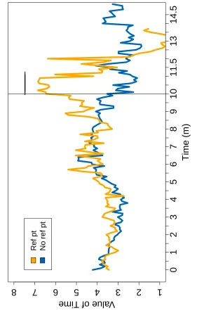
The above analysis was conducted with a particular reference point in mind. How-ever, the technique discussed can be used to not only measure the strength of loss aversion, but also to detect the location of reference dependence. Rather than divid-ing the data into pre- and post-reference point, I estimate time-use preferences in a sliding window. Displayed in Figure 2.13 is the 10% trimmed mean of the value of time in each group based on a 3-minute window for the period of time in which at least 3 individuals were active.8 The inferred preferences are relatively stable and comparable in both groups until the reference point is hit. At that point, the mean value of time among the remaining participants given the reference point sharply rises. The bar above the data denotes a statistically significant difference in group means at the 10% level according to a permutation test. Thus reference points can be identified from the data itself. Intriguingly, if I shrink the data window to 2 minutes, which increases the signal at the expense of noise, additional points of interest are revealed, shown in Figure 2.14. In particular, jumps are observed approximately halfway to and one minute before the reference point. Though not proposed be-forehand, the location of these jumps suggests that they may be benchmark effects. These timings are natural markers that could be used to set one’s pace, triggering changes in speed for those who feel they are behind.

An agent who takes advantage of benchmarks is behaving in a sophisticated fash-ion. Although there are hints of this occurring among inexperienced participants, individuals who have experience in the time allocation task may be better at pac-ing themselves. Figure 2.15 shows the distribution of completion times among

(34)

1

2

3

4

5

6

7

8 Estimated V

alues of Time

Time (m)

Value of Time

___

__

0

1

2

3

4

5

6

7

8

9

10

11.5

13

14.5

Ref pt No ref pt F

igure

2.13:

Mo

ving

a

v

erag

e

of

es

timated

v

alues

of

[image:34.612.159.450.183.628.2]

(35)

2

4

6

8

10 Estimated V

alues of Time

Time (m)

Value of Time

___

_

__

___

__

0

1

2

3

4

5

6

7

8

9

10

11.5

13

14.5

Ref pt No ref pt

F

igure

2.14:

Higher

resolution

mo

ving

a

v

erag

e

of

es

timated

v

alues

of

(36)

0 500 1000 1500

0.0000

0.0005

0.0010

0.0015

0.0020

Completion Time Distributions

Time (s)

Density

Given ref pt No ref pt Exp + ref pt

ref pt

Figure 2.15: Kernel density estimate of completion time data with experienced participants

experienced participants, which peaks before the reference point is hit. Further-more, the mean value of time shown in Figure 2.16, which accounts for changes in ability, is generally higher among those who are experienced, and peaks near the halfway point. These are not definitive markers of sophistication; they could stem from convexities in subjective cost due to fatigue or boredom from task repetition. Nonetheless, they are also consistent with forward-thinking agents, and suggest that reference dependence in time has the possibility to influence time allocation even outside of the loss regime.

(37)

2

4

6

8

10 Estimated V

alues of Time

Time (m)

Value of Time

0

1

2

3

4

5

6

7

8

9

10

11.5

13

14.5

Ref pt No ref pt Exp + ref pt

_

___

__

___

_

___

__

F

igure

2.16:

Mo

ving

a

v

erag

e

of

es

timated

v

alues

of

time

with

e

xper

ienced

par

(38)

0 5

10 15

Time Bef

ore First Completion Time (m)

Value of Time

−15

−13

−11

−9

−8

−7

−6

−5

−4

−3

−2

−1

0

F

igure

2.17:

Mo

ving

a

v

erag

e

of

es

timated

v

alues

of

time

with

e

xper

ienced

par

ticipants

relativ

e

to

firs

t

stag

e

completion

(39)

2.5 Conclusion

People often have beliefs about how long tasks will take to complete and become discontent if their expectations are violated. According to theories of reference-dependent preferences (e.g. Bell, 1985; Loomes and Sugden, 1986; Gul, 1991; Kőszegi and Rabin, 2006), people will try to avoid falling too far behind these expectations even if it means forgoing monetary payoffs. I conducted a real-effort experiment to test the theory’s predictions, finding support. Most directly, values of time more than doubled after participants exceeded the reference point based on external information, and work speed increased at the cost of reduced monetary earnings. Participant task completion times tended to cluster near the reference point. Those who fell behind were distinctly more dissatisfied, but not if they had prior experience in the task, suggesting that their reference points incorporated varied kinds of information. These findings strengthen the case for expectations-based reference dependence and the practical expansion of its domain to expectations in time.

My results apply to literatures on labor supply choices. I find evidence that the quantity and quality of labor supply are influenced by workers’ beliefs independent of a link to pecuniary outcomes. Theories of reference-dependent preferences predict that among workers with flexible daily hours, stopping probabilities are related to income earned in a given day. Several studies show this pattern (Camerer et al., 1997; Chou, 2002; Fehr and Goette, 2007; Doran, 2014; Leah-Martin, 2015), but observed levels of variation in earnings are not fully explained by a fixed earnings target (Camerer et al., 1997; Farber, 2005; Farber, 2008; Farber, 2015). Reference points assumed to be based on expectations in both time and money may, however, be able to account for this by admitting flexibility in response to contextual variation (Kőszegi and Rabin, 2006; Crawford and Meng, 2011). My study provides a check on these assumptions, and the results help justify use of the theory. My quantitative estimates of the strength of time-based loss aversion also accord with the closest figures in the empirical literature based on an alternative structural model, further validating a reference dependence approach.

(40)

(41)

C h a p t e r 3

A STATISTICAL TEST FOR THE OPTIMALITY OF

DELIBERATIVE TIME ALLOCATION

We are often tasked with choosing from multiple options. A subtle but essential part of the choice we make in selecting a job candidate or a consumer product is when to stop deliberating and pick an option. Such decisions involve an inverse relationship between speed and accuracy; we can make judgments that are fast but error-prone, or slow but high quality. Over the last half century, research in psychology and neuroscience has indicated a class of mathematical models of the deliberative process – diffusion models – that seem to well describe neural and behavioral data. However, while these models generate a speed-accuracy tradeoff, their applications are often agnostic as to how agents actually negotiate this tradeoff. One prominent hypothesis is that an agent’s stopping criterion optimally balances the costs and benefits of spending time.

Do people optimally balance the costs and benefits of time spent and accuracy attained? When conditions change, does behavior change commensurately? The answers to these questions are important because they inform us about how we can best generalize, predict, and influence a person’s behavior across various contexts. If people are behaving optimally, we can predict their behavior precisely using op-timization models even when task demands move outside of their original confines. If, on the other hand, people are not behaving optimally, then alternative models will furnish better predictions, and there may be room for interventions to improve the efficiency of decision making. For instance, time limits could prevent people from spending excess time on chronic deliberation between similar courses of action where deliberating yields little return.

(42)

In this paper, I propose a flexible way to test expected utility maximization in stochastic time allocation settings. This test can be applied in a variety of scenarios spanning perceptual tasks or value-based decision making. In tandem, I conduct experiments in the perceptual domain to investigate optimality according to the most well-known of diffusion models, the drift diffusion model. The experiments include both simple decisions, in which the agent knows the difference in values between better and worse choices, as well as more complex decisions, in which the value difference is uncertain. The latter involves the first test of new theoretical results by Fudenberg, Strack, and Strzalecki (2015) characterizing the optimal decision rule for the uncertain-difference drift diffusion model.

I find that when the value difference is known, a substantial fraction of participants do not appear to respond optimally to changes in task difficulty. Furthermore, when the value difference is uncertain, although the optimal decision rule provides an improvement over the standard fixed threshold assumption, participants do not appear to be sensitive to changes in monetary incentives. Thus there is still significant room for improvement in understanding the process of deliberation.

3.1 Background

(43)

of evidence accumulation processes that fit the model’s structure (Hanes and Schall, 1996; Shadlen and Newsome, 2001; Gold and Shadlen, 2002; Ratcliff, Cherian, and Segraves, 2003; P. L. Smith and Ratcliff, 2004).

Part of the DDM’s original motivation was its formal analogy with efficient sta-tistical algorithms. Importantly, the DDM was built as the continuous-time limit of the sequential probability ratio test (SPRT; A Wald, 1947) and is often theoret-ically characterized as inheriting its optimal stopping properties. For instance, it attains the speed-accuracy frontier (Abraham Wald and Wolfowitz, 1948; Arrow, Blackwell, and Girshick, 1949); that is, it achieves the highest accuracy for any given response time, and the quickest response time for any given accuracy level. Therefore questions of optimality bear upon the core identity of the model. We would like to understand how far the DDM’s optimality extends in practice.

To be more specific, in a two-alternative forced choice, the key outcomes about which decision makers are thought to care are time spent and performance attained. The former is penalized due to objective or subjective costs of time, and the latter is rewarded by association with some payoff. In the special but commonly encountered case that occurs when the rewards from the correct and incorrect options are fixed, performance reduces to accuracy, the probability of choosing the correct option. There are then two natural criteria for optimality based on these central elements.

The first criterion is to minimize a weighted sum of error rate and decision time, which is known as the Bayes Risk (Abraham Wald and Wolfowitz, 1948):

min

x∈X BR(x;y) = E R(x;y)+ψDT(x;y),

wherexandyare choice variables and fixed parameters, respectively, that determine the outcomes. The optimal choice depends on the free preference parameterψthat determines how much importance is placed on time relative to performance, and which may include a sizeable subjective component that is not directly observable. Thusψis interpretable as the subjective flow cost of time. The Bayes Risk expression is a special case of expected utility maximization when the reward depends only on whether the response is correct; more generally, the decision maker is assumed to solve maxx∈XE[r ewar d(x;y) −cost ×time(x;y)]. This is generally considered the most appropriate optimization criterion.

(44)

which is the Reward Rate (Gold and Shadlen, 2002):

max

x∈X RR(x;y)=

1−E R(x;y)

DT(x;y)+T0+D+E R(x;y)×Dp

,

whereT0is the time required for sensory and motor processing,Dis the time interval

between a correct response and the following stimulus, andDpis the additional time delay which penalizes an incorrect response on top ofD. This expression is relatively more common in psychology and ecology due to its origins in reinforcement rate analysis, but remains rarely used outside of those fields. The optimal choice here does not require the specification of any free parameters.

If the environment is homogeneous in difficulty, then the SPRT (and DDM) maxi-mizes any reward criterion based on error rate and decision time that is monotonically nonincreasing in decision time (Rafal Bogacz, E. Brown, et al., 2006). Thus the BR and RR optimal solutions happen to coincide perfectly. However, this is not the case in general. Because Reward Rate maximization is parameter-free, empirical tests of optimal choice have focused almost exclusively on this criterion (Simen et al., 2009; Rafal Bogacz, Hu, et al., 2010; Starns and Ratcliff, 2010; Starns and Ratcliff, 2012; Zacksenhouse, R Bogacz, and Holmes, 2010; Balci et al., 2011; Karşılar et al., 2014; Drugowitsch, Moreno-Bote, et al., 2012; Drugowitsch, DeAngelis, Klier, et al., 2014; Drugowitsch, DeAngelis, Angelaki, et al., 2015). Optimality in the Bayes Risk sense has thus been empirically neglected despite its theoretical importance.

(45)

That is, suppose one has data from two sets of problems, one with uniformly low difficulty and one with uniformly high difficulty. A person’s ability is likely lower among the high difficulty problems. The optimal decision rule in each set will be based on one’s ability and preference (for time versus accuracy). If we have reason to believe their preferences are the same across these sets (or at least hold some specific relation to each other), then the estimated decision rule in conjunction with the estimated ability in each set should imply the same preference across sets. This is the core of what is tested. While estimates of ability and decision rule will vary due to task difficulty, they should jointly indicate the same inferred preference if people are indeed optimally balancing the costs and benefits according to expected utility maximization.

Formally, as long as preferences can be identified using a type of likelihood estima-tion, consistency can be assessed using a likelihood ratio test where the restriction comes from the specified relation between preferences. In particular, if preferences are believed to be the same across multiple conditions, the restricted likelihood is based on equality between the preference parameters. Alternatively, weaker re-strictions based on inequalities can be made if one only wants to assume ordinal relationships between conditions.

This method is in the spirit of economic tests of revealed preference; it attempts to rationalize behavior under some specified theory without making any claims about the intrinsic reasonableness of possible preferences beyond basic consistency. This constitutes a relatively minimal standard for rationality – consistency is necessary but not sufficient, and failure to reject the null hypothesis of consistency is not definitive evidence that the agent is behaving optimally.

(46)

3.2 Variation in Difficulty

The choices we make often vary in their difficulty level. Some decisions are quick and obvious, while others are protracted and unclear. Can people optimally adjust their deliberative behavior according to the difficulty of decision problems? This ability is important for students taking their SATs or radiologists assessing the results of medical scans, all of whom must allocate time appropriately across easy and hard cases. I study this question in a common perceptual judgment paradigm, the random dot motion task, in which behavior and brain activity have been shown to fit the structure of the drift diffusion model.

Methods

In each trial of the random dot motion task, 100 white dots are displayed on a screen. As illustrated in Figure 3.1, a large fraction of them are “noise dots” moving in random directions (depicted as empty circles), while the remaining few are “signal dots” moving in a consistent direction (depicted as filled circles) –– either all to the left or all to the right. The agent must determine in which direction the signal dots are moving. This is a common task in perceptual decision making experiments (e.g. Newsome, Britten, and Movshon, 1989; Britten et al., 1992) and is straightforward enough that similar versions have been administered to a range of nonhuman animals including rats and mice (Douglas et al., 2006), pigeons (Nguyen et al., 2004), and rhesus macaques (Kim and Shadlen, 1999).

(47)

Figure 3.1: Schematic diagram of the random dot motion task stimulus

Essays on Timing and Economic Behavior

Rahul B. Bhui

ACKNOWLEDGEMENTS

ABSTRACT

TABLE OF CONTENTS

OVERVIEW

FALLING BEHIND: TIME AND EXPECTATIONS-BASED

REFERENCE DEPENDENCE

oppor

tunity

cos

t

(

π

)

oppor

tunity

cos

t

×

loss

a

v

ersion

(

λ

×

π

)

ref

erence

point

t

t

mar

ginal

benefit

per

tr

ial

w

a

(

t

)

ti

m

e

1

2

3

4

5

6

7

8

Estimated V

alues of Time

Time (m)

Value of Time

___

___

___

__

0

1

2

3

4

5

6

7

8

9

10

11.5

13

14.5

2

4

_point