A study of the application of paper spread function data to the prediction of physical dot areas for offset lithography

Rochester Institute of Technology

RIT Scholar Works

Theses

Thesis/Dissertation Collections

12-6-1986

A study of the application of paper spread function

data to the prediction of physical dot areas for offset

lithography

Paul Lewis

Follow this and additional works at:

http://scholarworks.rit.edu/theses

This Thesis is brought to you for free and open access by the Thesis/Dissertation Collections at RIT Scholar Works. It has been accepted for inclusion

in Theses by an authorized administrator of RIT Scholar Works. For more information, please contact

[email protected].

Recommended Citation

A

STUDY

OF

THE

APPLICATION

OF PAPER

~3F'h:Fr,U

F

'-I

I

,IC-'

1 Uhl

D(YU)

TO

THE

:

F'RED I CT I ON

Dr

F·HY

~'. T

U,L.

DDT

(:)r.:[

~,

~;

FDI:;:

DFFSET L

I

THOGRAF'H'!

'

b

y

F·

a.u.l E.. Lel,AJi s

B ..

S.

Vi~qinja

Pol

y

technic Institute

(197(3)

A

thesi

s

5ubmjtted

in

pa~ti2l

fulfillment

of th

e

~equi~ement5

for the

deg~ee

of

Ma

ster

of

Science

in

the

Cente~

for

Im

aging

Science in

the

Colle

ge

of

Graphic Arts

and

Photog~aphy

of

the

R

oche

~

ter

Institute of Technology

.Julle~

19136

Si

~lni

:

,tuT':o'

crf

tho:::~ {1Llthol~

_._

..

_

.

_

__

____________

~g!Jl.E.:..b~wi~

___ _

Cente~

fo~

Imaging Science

College of Graphic Arts and Photography

Rochester Institute of Technology

Rochester, New York

CERTIFIC

A

TE OF APPROVAL

M.S. DEGREE THESIS

The M.S. Degree Thesis of Paul E. Lewis

has been e

x

amined and approved

by the thesis committee as satisfactory

for the thesis requirement for the

Master of Science degree

Mr. Joe H. Altman, Thesis Advisor

Mr. Peter G. Engeldrum

Dr. Ronald Francis

---THESIS

RELE

ASE

PERMISSION FORM

RO

CHESTER INS

TITUTE OF TECHNOLOGY

COLLEGE OF GRAPHIC ARTS

AND PHOTOGRAPHY

Title

of thesis

B §IYQY

QE

I~~ BEEbl~BIIQ~

QE

EBE~B §EB~Bg

EY~~IIQ~

Q010

TO THE

EB~Ql~I!Q~

QE

E~Y§!~Bb

QQI

BB~B§

EQB

QEE§~I bII~99B8E~Y

D"

.

l

.

tE

~

E~~l

~~ ~~~i5, p~efe~

rep~oduction

is made.

A

STUDY

OF

THE

APPLICATION

OF

PAPER

SPREAD

FUNCTION

DATA

TO

THE

PREDICTION

OF

PHYSICAL

DOT

AREAS

FOR

OFFSET

LITHOGRAPHY

by

PAUL

EUGENE

LEWIS

Submitted

to

the

Center

for

Imaging

Science

in

partial

fulfillment

of

the

requirements

for

the

Master

of

Science

degree

at

the

Rochester

Institute

of

Technology

ABSTRACT

This

investigation

was

aimed

at

establishing

a

relationship

between

the

optical

spread

function

of

four

common

printing

stocks

(cast

coat,

enamel

gloss,

enamel

dull

and

ledger)

and

a

Yule

Neilsen

n

value

in

predicting

physical

dot

Area,

for

offset

lithographic

printing.

Using

an

offset

press

each

paper

stock

was

printed

with

a

test

target

containing

common

screen

frequencies

at

percent

dot

areas

from

5-90"/.

and

solid

ink

patches

adjacent

to

each

tint.

Using

planimetry

and

macrodensi

tometry

exact

n

values

were

calculated

for

comparison

with

the

measured

spread

function

of

that

same

paper

stock.

No

relationship

between

the

optical

spread

functions

of

the

printing

stocks

and

a

Yule

Neilsen

n

value

was

found.

Coated

stocks

(i.e.,

cast

coat,

enamel

gloss

and

enamel

dull)

behaved

differently

than

uncoated

stock

with

respect

to

n

VITA

Prior to entering the

graduate

program

in

Imaging Science,

I

worked

in

photo-finishing

laboratories for

six

years.

I

was

awarded

a

graduate

assistantship

by

the

Imaging

Science

Department

and

worked

for

two

consecutive

years

with

the

United

States

Navy

summer

training

program.

The

second

year

with

the United

States

Navy

summer

program

I

taught

color

theory

and

automated

printing.

In

addition,

I

worked

for

the

R.I.T.

photo-finishing

laboratory

as

a

technical

associate

and

laboratory

ACKNOWLEDGEMENTS

I

would

like

to

thank

the

following

people

for

sharing

their

experience,

and

donating

the

time

necessary

for

the

successful

completion

of

this

project:

Mr.

Joe

H.

Altman,

retired

Senior

Research

Associate

for

the

Eastman

Kodak

Co.,

who

as

my

thesis

advisor,

was

unbelievably

generous

with

his

time

and

effort

in

the

supervision

of

this

project;

Mr.

Peter

G.

Engeldrum,

of

the

R.I.T.

Center

for

Imaging

Science,

for

his

advice

and

enthusiasm;

Mr.

Milton

Pearson

of

the

R.I.T.

Research

Corp.,

for

his

technical

assistance;

and,

Mr.

William

Eisner

Director,

and

staff,

of

the

Technical

and

Educational

Center

of

the

Graphic

Arts

DEDICATION

This

thesis

is

dedicated

to

Ruth

and

Walter

Hess

whose

confidence

in

me

resulted

in

its

undertaking,

and

to

Claudia

whose

support

and

understanding

Table

of

Contents

SECJION

PAGE

#

Introduct

i

on

1

Exper i

mental

14

Results

27

Discussion

40

Conclusion

56

References

59

APPENDIX

A

Description

of

edge

projection

system.

62

APPENDIX

B

Controlling

program

for

Micro-densi tometer

65

APPENDIX

C

Program

that

calculates

spread

function

from

edge

gradient

data.

68

APPENDIX

D

Program

that

calculates

area

under

normalized

spread

function,

and

corrected

MTF.

71

APPENDIX

E

Materials

evaluated

in

measurement

of

system

MTF.

78

APPENDIX

F

Calculation

of

theoretical

system

MTF.

80

APPENDIX

G

Calculation

of

n

values.

84

APPENDIX

H

Linearity

comparison

of

TR927

and

M/M

densitometers.

91

APPENDIX

I

Calculation

of

dot

areas.

92

APPENDIX

J

Partial

derivatives

of

the

Yule

List

of

Tables

TABLE

CONTENTS

PAGE

1

Paper

stocks

and

basis

weights.

14

2

Parameters

describing

behavior

of

light

in

samples.

36

3

Average

basis

weight

and

thickness

for

press

sheet

and

additional

sample.

38

4-6

Analysis

of

variance

on

n

values.

41-42

7-8

Difference

in

percent

between

measured

and

predicted

areas

(cast

coat,

enamel

gloss,

enamel

dull)

and

(ledger).

46-47

9-11

Analysis

of

variance

on

para

meters

describing

sample

spread

functions.

49-50

12

Partial

derivatives

of

Yule

-Neilsen

equation

listed

in

order

List

of

Figures

FIGURE

CONTENTS

PAGE

1

Simplified

concept

of

light

inter

action

with

halftone

tint.

1

2

Repeating

rectangular

wave.

6

3

Test

pattern

layout.

18

4

Measurement

of

dot

area,

by

planimetry.

24

5-12

Graphs

of

edge

gradient,

spread

function

and

corrected

MTF

28-3'

for

all

samples.

13

Plot

of

n

value

as

a

function

of

measured

7.

dot

area

at

all

screen

frequencies.

38

14

Spread

function

comparison

for

all

Introduction

In

the

printing

industry

a

tone

scale

is

simulated

by

using

halftone

dots.

The

ability

to

reproduce

and

maintain

a

given

aim

density

(under

a

certain

set

of

press

conditions)

is

essential

to

quality

printing.

Varying

halftone

tint

density

is

accomplished

by

varying

the

dot

area

( 1 )

in

the

space

under

consideration

Maintaining

constant

tint

density

requires

a

quick

and

accurate

method

of

monitoring

the

dot

area

during

a

press

run.

In

the

printing

industry

today,

this

has

been

accomplished

to

a

great

extent

by

the

trial

and

error

application

of

an

n

value

to

the

Yule-Neil

sen

equation.

The

model

of

what

happens

to

light

as

it

interacts

(2)

with

a.

halftone

dot

pattern

is

a

very

complicated

one

Consider

a

checkerboard

pattern,

in

which

the

dot

area

is

507.,

on

a

white

paper

substrate.

It

should

absorb

less

than

507.

of

the

incident

light,

since

the

black

dots

never

totally

absorb

all

of

the

light

incident

on

them

(i.e.,

there

is

some

However,

such

a.

pattern

usually

absorbs

more

than

507.

of

the

incident

flux

and

reflectance

is

less

50%

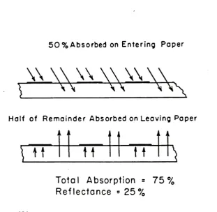
Absorbed

on

Entering

Paper

NX \\\N

\\

V,

N^

L\

I

Half

of

Remainder

Absorbed

on

Leaving

Paper

u

\

*t

ti

H

\

Total

Absorption

=75%

Reflectance

25%

Figure

(1)

Simplified

concept

of

light

interaction

with

a

halftone

tint.

(2)

Yule

and

Neilsen

conceptualized

the

interaction

of

light

with

a

halftone

reproduction

in

four

stages.

1.

Allow

one

unit

of

light

to

reach

the

reproduction.

Some

of

the

one

unit

is

reflected

back

(s),

and

(1-s)

is

not.

2.

(1-s)

is

transmitted

through

the

surface

and

dot

pattern.

As

a

result

a

fraction

proportional

to

the

dot

area

and

its

transmi ttance

is

absorbed

a*(l-Ts)

(where

Ts)

is

the

transmi

ttance

of

the

dot

and

a

is

the

dot

area).

This

is

what

is

available

to

the

paper

surface

(i.e.,

i-a*(l-Ts>

)

3.

A

fraction

of

i-a*(l-Ts)

is

absorbed

by

the

paper.

4.

That

which

is

not

absorbed

by

the

paper

is

diffused

by

it

and

after

internal

reflections

re-emerges

from

the

surface.

Here

it

again

takes

another

trip

through

the

dot

pattern,

which

again

absorbs

l-a*(l-Ts>.

(2)

According

to

Yule

and

Neilsen

the

fraction

of

incident

light

which

emerges

is

found

by

multiplying

all

the

above

events

together

and

adding

in

the

surface

reflectance.

This

results

in

the

following

equation

for

the

model

of

light

interacting

with

a

halftone

pattern

(the

equation

gives

the

reflection

of

a

macroscopic

area

of

a

halftone

pattern).

R=s+Rp(l-s) Cl-a(l-Ts) :

(1).

The

squared

term

denotes

two

trips

through

the

pattern.

Rp

is

the

reflectance

of

the

paper,

Ts

is

the

transmi ttance

of

For

practical

measurement

reasons,

equation

(1)

can

be

converted

to

contain

density

terms.

The

following

is

the

derivation

of

equation

(1)

in

terms

of

density

and

in

addition

the

reasoning

behind

its

further

transformation

from

the

Murray

-Davies,

to

the

Yule

Neilsen

equations.

Starting

with;

R

s+Rp (1-s) :i-a(l-Ts) 1

(1).

Rp

is

omitted

by

considering

the

density

of

the

paper

to

be

0. 0

(Rp=l)

thus,

R

s+(l-s)

Cl-a(l-Ts)

]

(2).

The

value

of

s

(the

surface

reflectance)

depends

on

the

gloss

of

the

paper

and

ink.

It

is

never

(according

to

Yule

and

Neilsen)

greater

than

0.04,

and

if

the

surface

is

very

glossy

it

may

be

disregarded,

leaving:

R

El-a(l-Ts) 1

(3)

If

a

1.0

equation

(3)

becomes:

Rs

Ts

or

1/2

Rs

Ts

Where

Rs

is

the

reflectance

of

the

solid

ink.

Converting

now

to

the

more

practical

density

form:

1/2

2

R

Cl-ad-(Rs)

) 1

(4)

Since

Ds

1/2

D

) D

(5).

1/2

Since

Ds/2

1/2

(-Ds/2)

1/2

=

log(Rs)

,

leaving

10

(Rs)

(-Ds/2)

1/2

By

substitution

of

10

for

Rs

in

equation

5,

we

now

arrive

at

the

Davies

equation:

D

-21ogCl-a(l-antilog

(-Ds/2) 1

(6).

(2)

Yule

and

Neilsen

substituted

a

compensating

factor

n

in

the

Murray-Davi

es

equation

to

make

the

calculated

results

more

closely

fit

the

observed

data

for

a

diffusing

substrate.

This

results

in

what

is

termed

the

Yule-Neil

sen

equation

:

D

-n

log

CI

log

(-Ds/n) 1

(7).

Equation

(7)

is

widely

used

in

the

printing

industry today

to

predict

the

density

from

the

physical

dot

area

of

a

halftone

print.

(3)

It

has

been

demonstrated

by

Pearson

that

the

value

of

n

depends

on

the

following

parameters

(listed

in

order

of

their

significance

in

contributing

to

the

value

of

n)

:

1.

The

spread

function

of

the

paper.

2.

The

halftone

screen

frequency

(v)

3.

Dot

area

(a)

4.

Solid

ink

density.

Because

the

Yule-Neil

sen

equation

is

based

on

such

a

simple

model

of

what

happens

in

a

halftone

print;

it

is

not

unless

a

correct

value

is

chosen

for

n

For

that

(4)

(5)

various

researchers

(Wakeshima

and

Kunishi

Lembeck

(6)

Ruckdeshel

and

Hauser

)

have

chosen

to

take

different

approaches

to

the

modelling

of

the

equation,

or

to

the

prediction

of

an

n

value

for

the

existing

equation.

The

Yule-Neil

sen

observation

that

light

entering

a

halftone

print

may

exit

at

another

point

has

been

(6)

characterized

by

Ruckdeshel

and

Hauser

in

terms

of

the

convolution

of

the

point

spread

function

of

paper

(i.e.,

uncoated

paper)

with

the

halftone

pattern.

This

gives

rise

to

the

following

equation:

I (x)

I(x')

)

d:

(8)

Where

indicates

the

position

of

the

incident

light,

x

represents

the

position

of

the

exiting

light,

1

)

represents

the

halftone

pattern

and

x7)

represents

the

point

spread

function.

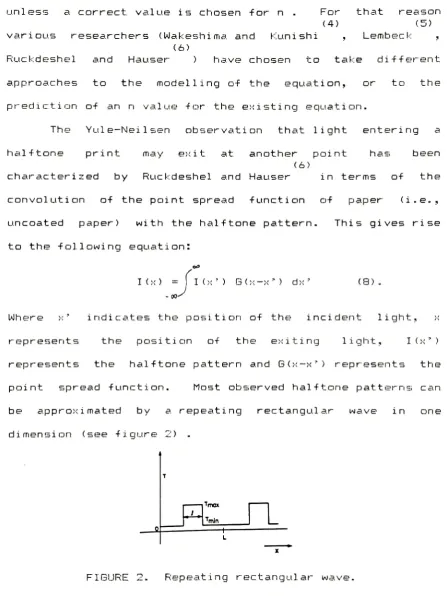
Most

observed

halftone

patterns

can

be

approximated

by

a

repeating

rectangular

wave

in

one

dimension

(see

figure

2)

,i_

Tmo

Tmln

(6)

For

this

reason

a

Fourier

series

representation

of

the

halftone

pattern

(see

equation

9)

can

be

substituted

for

I(x')

in

equation

(8).

T(x)

Tmin

+

(Tmax-Tmin)

m

1

2

*>

(-1)

mfM

2/fTmx

-

+

^>

sin

cos

L

/H"

mv=i

m

2L

L

(6)

(9)

Ruckdeschel

and

Hauser

have

also

reported

that

a

normalized

Gaussian

function

fits

observed

data

quite

well

for

an

uncoated

paper

spread

function,

G(x-x'),

and

is

of

the

form:

Gg(x-x')

exp[-(x-x')

/6

1

/fT6~

(10)

If

the

transmission

of

the

ink

layer

is

T(x)

and

the

incident

light

intensity

is

Io,

then

the

light

intensity

pattern

returning

from

the

paper

can

be

represented

as:

J (

x

)

T (

x)

f

la

oo-s

T(x' )G(x-x'

)dx

(11)

They

further

state

that

the

average

reflection

of

a

length

of

image

having

dimension

2x

becomes:

X

R

l/2x

/

J (x)dx

(12)

Substitution

into

equation

(11)

of

the

normalized

Gaussian

(i.e.,

equation

(10)

)

for

G

and

the

Fourier

series

representation

of

the

halftone

pattern

(i.e.,

equation

(9)

>

for

T

yields

the

light

intensity

pattern

for

a

screen

Ruckdeschel

and

Hauser

equation

for

the

of

a

screen

halftone

(see

equation

(13)

).

R

Cl-Ca(l-\/l

Rd) :

Ca(l-Ca)

\/Rd)

x

+

S

El-Cad-\/Rd)

1

(13)

Where

1 /L

line

repetition

frequency,

Ca

area

coverage

(i.e.,

1-1/L),

Rd

one

way

dot

transmi ttance

and

S

the

series

raitio

resulting

from

the

integration

of

equation

(11)

(see

equation

(14)

).

sin

(m-TTl/L)

m

exp[-(mTT6/L)

1

S

(14)

;in

(m-fTl/L)

m

Setting

equation

(13)

equal

to

the

Yule

-Neilsen

(i.e.,

equation

(7)

)

in

which

n

2,

an

improved

number

for

n

can

(6)

n

2.

log

\/pd)

1

1/n

log

(Rd)

)]

Ca

(1-Ca)

(1

vW

log

1

+

Cl-Ca(l

/Rd)]

1/n

log

El-Cad

-(Rd)

)

1

(15)

(6)

According

to

Ruckdeschel

and

Hauser

equation

(8)

may

be

simplified

for

screens

in

which

the

transmi ttance

of

the

dot

approaches

zero

(i.e.,

Rd=0)

and

for

small

area,

coverages

where

Ca

and

1

/L

both

approach

zero.

Under

this

condition

S

becomes

approximately

exp

"1T6/L)

where

i

s

the

paper

spread

function

width.

This

results

in

the

following

equation

for

the

improved

prediction

of

n:

n

2-exp

(-TT6*/L)

(16).

For

G

0.

1mm

the

values

of

n

show

a

good

fit

at

low

area

coverages

on

uncoated

paper.

For

high

and

middle

fractional

areas,

respectively,

equation

(8)

reduces

to

the

following

equati one:

n

2-CS/El+Ca(s-l)

11

(17)

n

(6)

Ruckdeschel

and

Hauser

based

on

their

argument

(presented

above)

and

experimental

results,

have

reported

the

following

information.

For

Xerox

4024

DP

paper,

the

Yule

Neilsen

equation

is,

in

principal,

adequate

in

approximating

the

relationship

between

average

reflection

density

and

area

coverage.

However,

since

n

becomes

increasingly

dependent

on

area

coverage

in

shadow

and

highlight

areas,

the

Yule-Neilsen

equation

should

not

be

used

for

prediction

in

these

areas.

Tone

reproduction

properties

as

affected

by

light

scattering

properties

can

be

specified

by

the

spread

function

di

stance.

The

distance

was

obtained

by

measuring

the

reflectance

profile

of

a

blackened

razor

edge

placed

in

close

contact

with

the

paper

substrate.

However,

no

reference

to

the

illumination

of

the

paper

substrate

was

given.

(7)

Yule,

Howe

and

Altman

have

reported

in

detail

about

a

device

for

measuring

the

spread

function

of

papers.

This

(8)

device

is

very

similar

to

that

of

F.C.

Eisen

The

very

important

difference

is

in

the

edge

that

is

projected.

Yule,

Howe

and

Altman

chose

to

use

a

low

contrast

edge

made

on

a

high

resolution

photographic

plate.

A

luminance

ratio

between

the

two

sides

of

this

edge

could

be

selected

so

that

it

is

within

the

linear

operating

range

of

the

instrument's

They

also

proposed

that

with

such

a

device

the

direct

measurement

of

the

spread

function

could

be

made

on

any

paper

stock.

The

basis

of

this

method

is

the

fact

that

if

a

knife

edge

is

projected

by

an

optical

system

onto

the

paper,

the

intensity

distribution

across

the

edge

is

equal

to

the

integral

of

the

line

spread

function.

E(x'

)=

f

A(x)dx

(19)

-ooJ

(7)

Yule,

Howe

and

Altman

have

suggested

that

if

the

spread

function

is

Gaussian

than

only

a

single

number

describing

its

width

is

an

adequate

description.

They

also

point

out

that

if

the

spread

function

of

the

instrument

is

not

narrow,

(measured

by

scanning

a

internal

ly diffusing

medium)

this

system

spread

function

should

be

removed

from

the

data.

Based

on

spread

function

measurements

made

on

their

scanning

device

and

the

printing

of

a

halftone

screen

test

target

on

four

papers

(baryta

coated,

titanium

dioxide

(7)

coated,

cast

coated,

and

uncoated)

Yule,

Howe

and

Altman

have

reported

the

following

results.

Reflection

densities

of

halftone

tints

were

highest

for

papers

with

the

widest

spread

functions

and

where

high

screen

frequencies

(i.e.,

greater

than

133

lines/in.)

were

used.

There

is

a

definite

correlation

between

the

width

of

the

spread

function

and

the

difference

between

the

equivalent

and

actual

dot

area.

Also,

the

change

in

tone

scale

due

to

light

spreading

is

screen

period.

This

causes

papers

with

wide

spread

functions

to

produce

higher

highlight

contrast,

darker

middletones

and

flatter

shadows.

It.

may

be

argued

that

the

Yule-Neilsen

model

is

too

simple

an

explanation

of

what

happens

to

light

in

a

halftone

print.

However,

the

Yule-Neilsen

equation

has

proved

(3)

adequate

in

predicting

the

relationship

between

reflection

density

and

physical

dot

area,

provided

the

correct

n

value

can

be

found.

The

principle

factors

in

contributing

to

n

are

the

following,

ranked

in

their

order

of

(3)

importance

:

1.

Paper

spread

function

2.

Halftone

screen

frequency

(v)

3.

Dot

area

(a)

4.

Solid

ink

density

(Ds)

Paper

spread

function

can

be

measured

using

a

device

similar

(7)

to

that

described

by

Yule,

Howe

and

Altman

Screen

frequency

does

not

change

as

a

result

of

the

offset

(9)

lithographic

printing

process

The

percent

dot

area

of

the

halftone

tint

can

be

measured

accurately

by

use

of

a

(9)

planimeter

Using

a

reflection

densitometer,

the

solid

ink

density

of

a

halftone

dot

can

be

determined

by

measuring

a

large

enough

area

of

printed

solid

ink

adjacent

to

the

(9)

halftone

tint

under

consideration

The

objective

of

this

research

(using

the

above

measured

optical

spread

function

of

four

common

printing

stacks

(cast

coated,

enamel

gloss,

enamel

dull

and

ledger)

and

a

Yule

Neilsen

n

value

in

predicting

physical

dot

area

lithographic

printing.

By

establishing

this

relationship,

n

values

can

be

determined

for

paper

stacks

prior

to

offset

lithographic

printing

by

measurement

of

their

optical

spread

functions.

Since

the

Yule

-Neilsen

equation

affords

quick

and

accurate

dot

area

calculation,

provided

the

correct

n

value

is

used,

dot

gain

could

then

be

monitored

during

a

EXPERIMENTAL

PAPER

SAMPLES

Table

(1)

lists

the

four

paper

stocks

used

in

this

experiment

along

with

their

basis

weights.

PAPER

STOCK

BASIS

WEIGHT

(GRAMS /SQUARE

METER)

cast

coat

(MFG)

190

enamel

gloss

(MFG)

95

enamel

dull

(MFG)

103

ledger

(MFG)

93

Table

(1).

Paper

stocks

and

basis

weights.

APPARATUS

Paper

edge

gradient

measurements

were

made

on

a

Xerax

scanning

reflection

Macro/Micro

densitometer

located

in

the

Microdensi

tometry

Laboratory

of

the

Rochester

Institute

of

Technology.

The

following

is

a

general

description

of

the

components

of

this

instrument:

1.

A

focusable

head

which

contains

the

following:

a)

A

pellicle

mirror

and

ground

glass

for

focusing

the

instrument

on

the

sample.

b)

A

NA

lens

for

the

collection

of

reflected

flux

from

the

sample.

c)

A

PMT

(photomul

tipl ier

tube)

is

used

for

detection

of

the

reflected

flux.

apertures.

e)

A

cylinder

containing

a

variety

of

filters

that

can

be

placed

between

the

PMT

and

its

incident

flux.

2.

The

signal

from

the

PMT

is

conducted

by

shielded

cable

to

a

housing

containing

the

following

components:

a)

An

analog

to

digital

converter

for

digital

signal

readout

from

the

PMT.

b)

Gain

controls

for

the

calibration

of

the

instrument.

c)

A

logging

circuit

for

digital

density

readings.

3.

A

scanning

stage

is

located

directly

beneath

the

instrument

head

and

contains

the

following

components:

a)

A

flat

surface

upon

which

the

sample

is

placed.

b)

Stepping

motors

which

control

the

X-Y

movement

of

this

stage.

The

movement

of

the

stage

and

collection

of

data

is

controlled

by

a

Wang

computer

interfaced

to

the

instrument.

The

following

modifications

have

been

made

to

this

(10)

instrument

since

its

use

by

Brian

T.

Pridham

:

1.

An

RCA

1P21

photomul

ti

pi

i

er

tube

was

installed

replacing

the

original

Hamamatsu

R446.

This

tube

is

more

sensitive,

allowing

greater

range

in

the

measurement

of

reflected

flux.

2.

The

scanning

stage

(originally

flat

white)

has

been

painted

flat

black

to

eliminate

reflection

from

the

stage

back

through

the

sample.

3.

A

special

illuminating

system

for

the

projection

of

a

low

contrast

edge

has

been

mounted

on

the

scanning

stage.

This

edge

was

made

from

a

Kodak

High

Resolution

Plate

with

a

transmission

ratio

from

light

to

dark

of

10:1

(see

appendix

A

for

detailed

description).

4.

A

Kodak

Wratten

#58

filter

was

mounted

between

the

PMT

and

its

incident

flux.

This

replaces

the

narrow

banded

(530nm,

14nm

bandpass)

green

filter.

This

increased

the

operating

range

and

signal

to

noise

ratio

of

the

i

nstrument

EXPERIMENTAL

PROCEDURE

Sample

Measurement

on

Xerox

Macro/Micro

Densitometer:

From

a

500

sheet

batch

of

each

stock

(i.e.,

cast

coated,

enamel

gloss,

enamel

dull

and

ledger)

edge

gradient

measurements

were

made

on

the

following:

1.

The

actual

press

sheet

containing

the

printed

halftone

test

target.

2.

An

additional

sheet

of

the

same

stock

for

comparison

to

the

press

sheet

measured

above.

The

procedure

for

edge

gradient

measurements

is

as

follows:

1.

The

optical

system

of

the

reflection

mi

crodensi

tometer

was

focused

on

the

paper

sample.

2.

The

projection

system

was

then

aligned

with

the

optical

system

of

the

densitometer.

projection

focus

positions

and

the

scan

with

the

steepest

edge

gradient

was

selected

as

of

the

paper

sample.

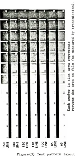
Printing

of

Halftone

Paper

Samples:

A

ByChrome

Percentage

Scale

on

Film

was

used

to

make

the

printing

plate

from

which

the

test

pattern

was

printed.

This

percentage

scale

on

film

consisted

of

the

following:

1.

Halftone

dot

screens

of

150,

133,

120,

110,

100,

85

and

65

lines/inch.

2.

Each

of

the

above

screens

has

a

range

of

percent

dot

areas

from

5-907..

The

paper

stocks

were

printed

on

a

Heidelberg

M0ZP

19

X

offset

lithographic

press

using

Marathon

Hard

Dry

Black

ink.

From

the

printed

halftone

test

pattern

n

values

were

calculated

for

the

following

tints,

on

all

four

paper

stocks

(see

figure

3

for

test

pattern

layout):

1.

Line

screens

of

150,

133,

100

and

65

lines/in..

+

0uj M"J

OS

o!J

o!

K

Z

coZ

esZ

Z

oZ

-3

'"-J

"-!

""-<

LU Ul

DATA

COLLECJION

Edge

Gradient

Measurements:

The

stepping

motor

on

the

Xerox

Macro/Micro

densitometer

is

computer

controlled.

A

scanning

program

was

written

to

take

advantage

of

this

feature.

The

program

finds

the

projected

edge

on

the

instrument

stage,

backs

off

and

then

scans

the

edge

averaging

10

readings

at

each

sample

position

(see

appendix

B

for

program

listing).

Because

the

sample

positions

are

fixed

at

.0127mm

apart,

a

scanning

aperture

of

1

X

was

selected.

This

is

equivalent

to

(11)

sampling

at

the

Nyquist

Interval

According

to

Shannon's

sampling

theorm

the

sampling

interval

/^X

should

be

the

(11)

following

:

AX

^

l/2Umax

(20)

The

maximum

spatial

frequency

(i.e.,

Umax)

that

can

be

imaged

by

the

selected

scanning

aperture

(i.e.,

1

X

is

40

cycles/mm.

Substitution

of

this

value

for

Umax

in

the

above

equation

allows

for

the

fixed

stepping

increment

of

For

the

purposes

of

establishing

a

relationship

between

the

spread

function

of

each

sample

and

a

Yule

-Neilsen

n

value,

a

quantitative

description

of

the

behavior

of

incident

light

in

each

sample

is

needed.

The

following

paragraphs

describe

the

three

quantitative

values

used

and

how

they

were

Corrected

Spread

Function

Width:

From

the

reflection

edge

gradient

the

derivative

(i.e.,

slope)

between

each

step

was

calculated

by

a

computer

program

using

equation

(21)

(see

appendix

C

for

computer

program

listing).

Ders(I)

(Edge ( I )

-Edge

(1+1 ))/. 0127

(21).

Where

Edged)

is

an

array

containing

the

reflectance

edge

gradient

data

and

Ders(I)

is

an

array

containing

the

calculated

derivative

between

consecutive

edge

gradient

sample

positions.

By

definition,

the

array

Ders

contains

the

uncorrected

sample

spread

function.

This

array

was

then

normalized

(i.e.,

each

value

for

Ders ( I )

was

divided

by

the

value

at

Ders(I)max.)

resulting

in

the

uncorrected

normalized

sample

spread

function.

This

uncorrected

normalized

sample

spread

function

contains

the

convolution

of

both

the

paper

and

instrument

spread

functions.

The

width

of

the

convolutions

of

two

functions

is

approximately

the

sum

of

the

(11)

two

widths

Therefore,

the

width

of

the

scanning

aperture

(i.e.,

was

subtracted

from

the

width

of

the

uncorrected

spread

function.

This

was

used

as

the

corrected

spread

function

width.

Area

Under

Uncorrected

Spread

Function:

The

uncorrected

normalized

sample

spread

function

was

then

truncated

at

a.

point

on

either

side

of

the

actual

edge

discrete

Fourier

Transform

DFT

(see

appendix

D

for

computer

program

containing

DFT).

Equati

on

(22)

shows

the

definition

of

the

Fourier

Transform

using

the

uncorrected

normalized

sample

spread

function,

unssf.

-(i2/ftvx>

UNSSF (v)

unssf

(x)

exp

dx

(22).

Where

UNSSF

(v)

Fourier

Transform

of

the

normalized

sample

spread

function

unssf

(x)

and

v

spatial

frequency

(i.e.,

cycles/mm).

A

computer

program

using

a.

Fast

Fourier

Transform

calculates

discrete

Fourier

Transform

values

of

UNSSF

(v)

(see

appendix

D

program

listing).

The

criterion

used

to

truncate

the

spread

function

is

as

foil

ows:

1.

Approaching

the

edge

the

spread

function

was

truncated

at

the

first

point

where

the

derivative

approaches

zero

and

previous

derivatives

are

no

greater

than

points

well

ahead

of

the

projected

edge.

2.

After

passage

of

the

edge

the

spread

function

was

truncated

at

the

first

point

where

the

derivative

approaches

zero

and

subsequent

derivatives

are

no

greater

than

points

well

behind

the

projected

edge.

The

area

under

the

uncorrected

normalized

spread

function

is

equal

to

the

integrated

reflectance

across

the

projected

edge.

According

to

the

Central

Ordinate

property

of

Fourier

(11)

Transforms

;

the

area

under

this

uncorrected

normalized

equal

to

the

central

ordinate

of

its

Fourier

Transform.

Therefore,

this

quantitative

value

was

used

for

its

ease

in

comparison

of

relative

differences

in

the

integrated

reflectance

across

the

projected

edge

between

different

paper

samples.

Spatial

Frequency

at

407.

Corrected

MTF:

Because

of

the

difficulty

in

finding

a.

material

that

would

be

an

ideal

diffuse

reflector

with

no

internal

scatter

and

high

reflectance,

the

actual

system

(i.e.,

edge

progection

system

and

Xerox

Macro/Micro

densitometer)

spread

function

could

not

be

measured

(see

appendix

E

for

materials

tried).

The

Fourier

Transform

of

the

uncorrected

normalized

sample

spread

function

UNSSF

contains

the

Fourier

Transform

of

both

the

paper

sample

and

the

system.

To

find

the

Fourier

Transform

of

just

the

paper

sample,

the

theoretical

MTF

(Modulation

Transfer

Function)

of

the

system,

SYSMTF,

was

removed

from

UNSSF

in

frequency

space

by

division.

The

following

paragraphs

describe

how

SYSMTF

was

calculated

and

removed

from

UNSSF

resulting

in

the

corrected

MTF.

The

theoretical

MTF

of

each

lens

in

the

system

(i.e.,

.08

NA

projection

lens

and

NA

collection

lens)

were

(12)

calculated

using

the

Hufnagle

formula

for

a

diffraction

limited

lens

at

530nm

(i.e.,

peak

transmission

wavelength

of

the

Wratten

#58

filter).

This

formula

was

used

instead

of

the

actual

formula

since

its

accuracy

is

actual

values

and

affords

much

easier

MlF

I

he

formula

i

s

as

follows:

4

Ta(w)

1

1.25(w/w0)

+

0.25(w/w0)

(23).

where

w

radius

frequency

and

wO

2NA/

.

00053mm.

The

Fourier

Transform

of

the

scanning

aperture

and

its

resultant

MTF

were

calculated

by

the

sine

(,025v)

(24)

where

v

spatial

frequency

(cycles/mm),

scanning

aperture

width

in

mm

and

sinc(.025v)

the

following:

sin

CiT.025v)

sinc(.025v)

(25).

"fT

025v

Because

an

optical

system

can

be

considered

a

linear

system,

the

MTF

of

the

entire

system

SYSMTF

can

be

calculated

by

the

product

of

the

individual

MTF's

frequency by frequency

(see

appendix

F

for

calculations).

The

corrected

MTF

was

obtained

by

complex

division

in

frequency

space

in

the

manner

described

by

equation

(26")

(see

appendix

D

for

computer

program).

Corrected

MTF(v)

(26)

UNSSF (v)

SYSMTF

(v)

The

frequency

at

which

the

corrected

MTF

0.4

is

the

value

reported

as

Spatial

Frequency

at

407.

corrected

MTF.

Calculation

of

Exact

n

Value:

From

the

printed

samples

the

following

measurements

were

made

and

applied

to

the

Yule

Neilsen

equation

to

obtain

the

exact

n

value.

1.

In

order

to

measure

by

planimetry

the

desired

tint

areas

the

following

procedure

was

used:

a)

Photomicrographs

were

made

on

Polaroid

film

type

52

using

a

Nikon

OPT I PHOT-POL

microscope.

b)

The

following

magnifications

were

used

to

get

four

to

six

dots

on

a

sheet

of

film.

Screen

freq.

lines/in.

Magnification

150,

133

200 X

100

160X

65

100X

c)

Concentric

circles

were

used

to

find

the

center

of

each

dot.

The

centers

were

connected

by

fine

tip

ink

pen

d)

The

dots

and

areas

inside

the

connected

concentric

circles

were

measured

by

planimetry.

The

measured

area

resulting

from

the

connection

of

the

centers

of

the

dots

was

used

as

the

unit

area.

Percent

dot

area

was

obtained

through

the

division

of

the

combined

measured

dot

areas

by

the

unit

area

(see

figure

4).

2.

A

K&E

Compensating

Polar

Planimeter

was

used

to

measure

the

dot

and

unit

areas.

3.

Tint

density

was

measured

on

a

Macbeth

TR

927

reflection

densitometer

(using

the

green

Wratten

#61

filter).

This

filter

was

used

because

its

transmi ttance

measure

the

edge

gradients

of

the

4.

Solid

ink

densities

were

also

measured

on

this

instrument,

with

the

Wratten

#61

filter.

5.

The

Yule

Neilsen

equation

was

used

with

the

above

measured

areas

and

densities

to

calculate

an

exact

n

value

(using

iteration)

for

the

sample

tint

in

question

(see

appendix

G,

calculation

of

n

values).

_UnL_ax.a.

Figure (4)

Measurement

of

Percent

dot

area

by

planimetry.

LINEARITY

OF

THE

MACBEJH

AND

XEROX

M/M

DENSITOMTTERSl

To

that

the

low

contrast

edge?

(mentioned

in

the

apparatus

section)

with

its

transmission

ratio

of

10:1

would

be

within

the

linear

range

of

Xerox

M/M

densitometer

and

that

both

instruments

were

operating

in

a

linear

range,

the

following

procedure

was

used:

range

to

cover

107.

transmission

(i.e.,

reflection

density

of

1.0

or

greater)

was

measured

on

both

instruments.

2.

The

density

measurements

from

the

Macbeth

TR

927

were

plotted

against

the

percent

maximum

reflectance

readings

taken

on

the

Xerox

M/M

densitometer.

The

results

showed

a

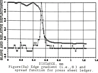
RESULTS

Figures

5-12

contain

graphs

of

the

reflection

edge

gradient,

uncorrected

normalized

spread

function

and

corrected

MTF's

for

the

press

sheet

and

additional

sample

of

each

paper

stock

(i.e.,

cast

coat,

enamel

gloss,

enamel

dull

O.i

0.8

11

1-

14

DISTANCE,

mm

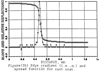
Figure

(5a)

Edge

gradient

(i.e.,n)

and

spread

function

for

press

sheet

cast

coat

m

ted

""ill

L

^^Skno-(

11

"

i

'

I

LAJ&

*\

mTttlllMlJ,,,

J

\

' ' ' '

O.i

04

0.1

0.8

11

tl

14

DISTANCE,

mm

m

DQfl

Is

is

S

58*

ari^****"***3

^tHH+^H3^;

^

^

i

( m

ad^

iw

W-

A

Y

1

O.I

04

0.0

0.8

1

?.S

14

DISTANCE,

mm

Figure

(6a)

Edge

gradient

(i.e.,

a)

and

spread

function

for

press

sheet

enamel

^loss

0Q0

oy

=3

KM

<H4

s3?

I^Wriri"^

ifcgfrf^

i

-hi

-\

A

AooT1

a

l]

k

AuLiiiua

;

VV\r

0.1

04

0.0

0.8

11

1.S

DISTANCE,

mm

Figure(6b)

Edge

gradient

(i.e.,D)

and

spread

function

for

enamel

gloss.

o.s

04

0.0

0.8

D

1.1

14

DISTANCE,

mm

Figure

(7a)

Edge

gradient

(i.e.,D

)

and

spread

function

for

press

sheet

enamel

dull

m

(3

m

ii

3'

2^

yW

^

i

miHlumPfr

Um

M

!

1 '

0.1

04

0.0

0.8

DISTANCE,

mm

Figure(7b)

Edge

gradient

(i.e.,0)

and

m

Hi**

DBS

|2

DGfl

S3

2

<l\l>

^JU

'h

*

w

!

fem

uw

* ' '

'

0.1

04

0.0

0.8

11

tl

DISTANCE,

mm

Figure(3a)

Edge

gradient

(i.e.,D)

and

spread

function

for

press

sheet

ledger

14

DISTANCE,

mm

Figure

(8b)

Edge

gradient

(i.e.,n)

and

o '

-P^n

\

s,

\

\

2

o

1-1.1

0

7.1

10

11.1

II

17.0

10

U.I

10

SPATIAL

FREQUENCY

Figure

(9a)

Corrected MTF

for

press

sheet

cast

coat

7.1

HO

12.1

tl

17.0

10

U.I

SPATIAL

FREQUENCY

s

-e

-3

5

0"

o-

_-7.1

10

11.1

11

17.1

10

U.I

U

SPATIAL

FREQUENCY

Figure

(10a)

Corrected

MTF

for

press

sheet

enamel

gloss

0 '

\

**

e

-\,

3"

2

o-0

I

10

HI

10

II

SPATIAL

FREQUENCY

Figure(lOb)

Corrected

MTF

for

enamel

gloss.

4

2

LW^I

I

I

I

1

I

I

SPATIAL

FREQUENCY

Figure

(11a)

Corrected

MTF

for

press

sheet

enamel

dull

4

2

SPATIAL

FREQUENCY