KNOTS, SATELLITES AND QUANTUM GROUPS
H. R. Morton
Department of Mathematical Sciences, University of Liverpool Peach Street, Liverpool L69 7ZL
Keywords: satellite; Homfly polynomial; skein; annulus; quantum invariant
1. Introduction
These notes are an expanded version of a series of lectures given in ICTP Trieste and at Universidad Complutense, Madrid in April and May 2009.
They are primarily an account of knot and link invariants derived from the Homfly polynomial by the use of satellites. They are based mainly on work by myself and former students at Liverpool University. Much of this can be found in greater detail through the Liverpool University knot theory publications list, including the doctoral theses of Aiston, Lukac and Hadji. I refer readers also to an extended expository article11 where a similar approach, focused more on satellite invariants for the Jones polynomial, is adopted. This article contains earlier work on the Homfly invariants, which culminated in two papers with Aiston.2,13
More recent papers are those on the Murphy operators9,10 and work with Lukac and Hadji3,7,14, where the technique of using the meridian maps has been developed and refined. The latest paper with Manchon15gathers together results about the Homfly skein of the annulus, which is the prime tool for organising satellite invariants.
1.1. Setting the scene
We are all able to tie a knot in a piece of rope. The pictures in figure 1 show some examples.
What exactly do we mean though when we say that a piece of rope is knotted?
Fig. 1.
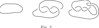
[image:2.595.197.396.265.323.2]as in figure 2. Compare what happens in the three cases.
Fig. 2.
In the first case we get a simple, or ‘unknotted’ circle, while in the second case we have a circle with what appears to be a knot in it.
Let us say that the rope isknottedif no possible manipulation of it will result in the unknotted circle. We do not allow cutting and rejoining.
The third example can clearly be undone by a little manipulation to form the simple circle, so again the rope is unknotted.
We model this notion of a knot mathematically by referring to a closed curve inR3as a knot, with the special case of the simple circle, lying say as the unit circle in a plane, known as thetrivial knotorunknot. Knot theory in the mathematical sense is then the study of closed curves in space.
We call two knotsequivalentif one can be manipulated, without passing one strand through another, to become the other knot. I give a more formal technical description of this below, but essentially anything is allowed which could be done with a rather stretchable piece of rope. The one manoeuvre which must be excluded is the analogue of the bachelor’s technique for ignoring knots on a piece of cotton – pull it so tight that you can hardly see it! Using this technique on a curve with no physical thickness would get rid of any knot.
We would like to know for a start if there are any knots which are not equivalent to the trivial knot. If so, are there lots of different knots, and how might we distinguish between them?
It is easy to imagine that you have been given two knots and by a little patient work you manage to manipulate one to look like the other, e.g. the first and third knots in figure 2. What happens though if you find that even after a lot of trying you can’t make them look the same – does it follow that the knots are inequivalent, or have you just not been dextrous enough? There is clearly a problem here, and something else will be needed, as there is no way that failure to manipulate can show that it is actually impossible to do so.
It should be realised that the question of how the rope is knotted isn’t an intrinsic question about the rope alone, but rather a matter of how the rope is placed in space. Every closed loop of rope looks the same to an ant inside the rope. Some of the techniques developed for the study of knots have proved fruitful in other ‘placement problems’, i.e. in studying the different ways in which one particular geometric object, here a closed curve, may lie inside a larger one.
1.2. Background
The idea of looking at knotted and unknotted closed curves goes back to Gauss and beyond. Kelvin had some idea of trying to relate different types of atoms to knotted curves in the ether; this was taken up by a Scottish physicist Tait, who set out to enumerate all possible different knots in the hope of tallying them against different atoms. His lists of knots soon showed that the task of systematically enumerating all knots was hopelessly complicated; among other problems there are infinitely many. It is still true today that no practical framework exists for producing a comprehensive list, although Thistlethwaite has devised a fairly good means of handling the simpler knots. Various mathematicians in the 1920s and 1930s developed methods to show up a number of general properties shared by all knots, using some very elegant geometrical techniques and exploiting the growing interplay between algebra and this style of geometry. From this period has come the Alexander polynomial, and interpretations of it, as well as group theoretic invariants. Much more recently knot theory and theoretical physics have again had close contacts.
Definition 1.1. Aknotis a simple closed curveK⊂R3or inS3.
We shall only deal with tame knots, e.g. smooth or polygonal curves, and we assume thatK has a solid torus neighbourhoodV with
(V, K)∼= (S1×D2, S1× {0}).
This is like insisting on using a piece of rope, although one whose exact thickness will not matter.
It is often convenient to deal with S3−intV = extK, the exterior of K, which is a compact 3-manifold with boundary ∂(extK) = ∂V ∼=
torusS1×S1.
From the point of view of topological invariants there is not much dif-ference betweenS3−K, extK andS3−V.
Definition 1.3. Knots K0 and K1 are homeomorphic if there exists a homeomorphismh:R3→R3 such thath(K0) =K1.
Ifhis orientation preserving we can deformK0toK1through a family of knotsKt =ht(K0). We shall callK0 and K1 equivalentwhen they are related in this way. (The termambient isotopicis also used.)
Conversely a 1-parameter sliding of a neighbourhoodV ofK0to one of
K1 throughR3 can be extended to such a family htof homeomorphisms, and models quite well the physical notion of equivalence by manipulation of a closed loop of rope.
We then have the result, by composing with a reflection if necessary, that two knotsK0andK1 are homeomorphic if and only ifK0 is equivalent to
K1or its mirror-image.
Remark 1.1. Some knots, for example the trefoil, are not equivalent to their mirror image, while others such as the figure-eight knot are.
1.3. Knot diagrams and moves
For our subsequent analysis we concentrate on tame knots, i.e. knots equiv-alent to finite polygonal curves or equally to regular smooth curves.
Diagrams connected by a sequence of Reidemeister’s moves, seen in figure 4, represent equivalent knots.
The converse is also true.
Theorem 1.1 (Reidemeister). If two diagrams represent equivalent
I R
II R
[image:5.595.248.342.159.264.2]III R
Fig. 4. Reidemeister’s moves
1.4. Links and linking number
We may enlarge our scope slightly and look, as Gauss did, not just at a single closed curve but at several at once.
Definition 1.4. Alinkofrcomponents is a collectionL=L1∪L2∪. . .∪Lr ofrclosed non-intersecting curves.
Whenr= 1 we have a knot. In the caser= 2 we can very simply associate an integer with a link, which is the same for every equivalent link. This is called thelinking numberof the two components.
To define the linking number lk(L1, L2) we must first choose an orien-tation of each of the components, which we note on a diagram of the link by drawing arrows on the curves. Now look at one diagram of the link and consider only the crossings whereL1 crosses overL2. Each of these cross-ings ci can be given a sign εi = ±1, according to a conventional choice. The sum of these signsPεi is unaltered when the diagram is changed by Reidemeister moves. For crossings ofL1overL2 are not affected by moves I and III, while if there are any involved in a move of type II they occur as a pair with opposite sign, so that the sum is unchanged.
Reidemeister’s theorem holds also for links. We may then set lk(L1, L2) =Pεi for any choice of diagram.
Proposition 1.1. lk(L2, L1) =lk(L1, L2).
Proof. To calculate lk(L2, L1) we must count the crossings ofL2over L1 in some diagram. Start with a diagram in which we count the crossings
this diagram is identical to the sum calculating lk(L1, L2) in the original diagram.
1.5. Framed links
Framed links are made from pieces of ribbon rather than rope, so that each component has a preferred annulus neighbourhood. Combinatorially they can be modelled by diagrams inS2 up toR
II andRIII, excluding RI, by use of the ‘blackboard framing’ convention. The ribbons are determined by taking parallel curves on the diagram.
Reidemeister moves II and III on a diagram give rise to isotopic rib-bons. Any apparent twists in a ribbon can be flattened out using Reide-meisterI.
Oriented link diagrams D have awrithe w(D) which is the sum of the signs of all crossings. This is unchanged by movesII andIII.
For a framed knot the writhe is sometimes called its ‘self-linking num-ber’, which is independent of the orientation of the diagram. Generally a framing of a link is determined by a choice of writhe for each component.
1.6. Satellites
A satellite of a framed knotK is determined by choosing a diagramQ in the standard annulus, and then drawingQon the annular neighbourhood ofKdetermined by the framing, to give the satellite knotK∗Q. We refer to this construction asdecorating K with the pattern Q(see figure 5).
[image:6.595.138.440.495.571.2]Q= K= K∗Q=
Fig. 5. Satellite construction
It is often possible to use satellites with some fixed choice of patternQ
The Conway polynomial∇(K) is not useful in this context, since
∇(K∗Q) =∇(K′∗Q)
for every choice ofQ, if∇(K) =∇(K′).
This limitation does not hold in general. In particular the extension of the Conway polynomial known as the Homfly polynomial will often give useful extra information when applied to satellites.
Remark 1.2. The use of satellites is sometimes known ascabling. I prefer to reserve the term ‘cable’ for satellites where the patternQ is based on some (p, q) torus knot.
2. Homfly invariants
In 1984 V.F.R.Jones constructed a new invariant of oriented linksVL(t)∈
Z[t±1
2], which turned out to have the property that
t−1VL+−tVL− = (
√
t−1/√t)VL0
where the links
L+ = , L−= , L0=
differ only as shown. This was quickly extended to a 2-variable invariant
PL(v, z)∈Z[v±1, z±1], with the property that
v−1PL+−vPL− =zPL0.
The name ‘Homfly polynomial’ has come to be attached to P, being the initial letters of six of the eight people involved in this further development. The polynomialP contains both the Conway/Alexander polynomial, and Jones’ invariant, and can be shown to contain more information in general than both of these taken together. We have
P(1, z) =∇(z)
P(1, s−s−1) = ∆(s2)
P(s2, s−s−1) =V(s2)
P(s, s−s−1) =±1
Given the existence of V and P we can then make some calculations. For example, the unlink with two components has
P = v −1−v
z ,
V(s2) =−(s+s−1),
while the Hopf link with linking number +1 has
P =vz+ (v−1−v)v2z−1,
V(s2) =s3−s−(s+s−1)s4=−s(1 +s4).
The Hopf link with linking number−1 has
P =−v−1z+ (v−1−v)v−2z−1, V(s2) =−s−1(1 +s−4).
This illustrates the general feature that for the mirror image L of a link
L, (where the signs of all crossings are changed), we have PL(v, z) =
PL(v−1,−z) and soV
L(s2) =VL(s−2). It is thus quite possible to useV in many cases to distinguish a knot from its mirror-image, while there will be no difference in their Conway polynomials. It is worth noting that although there are still knots which cannot be distinguished from each other byP
in spite of being inequivalent, no non-trivial knot has so far been found for whichP = 1, or evenV = 1.
The original Homfly polynomial is invariant under all Reidemeister moves, but there is a convenient version which is an invariant of a framed oriented link
In its most adaptable form, PL(v, s), it lies in the ring
Λ =Z[v±1, s±1,(sr−s−r)−1], r >0.
Its defining characteristics are the local skein relations.
(1) − = (s−s−1)
(2) = v−1 , = v .
These relate the invariants of links whose diagrams differ only locally as shown.
They are enough to allow its recursive calculation from simpler diagrams in terms of the value for the unknot.
The local nature of the skein relations between invariants allows us to make a useful simplification in studying them.
Compare for example three patternsQ± andQ0.
Q+= ,Q−= ,Q0= .
The framed Homfly invariants ofK∗Q± andK∗Q0 then satisfy
P(K∗Q+)−P(K∗Q−) = (s−s−1)P(K∗Q0).
Since K∗Q− is the unknot for any K, this relates the invariants of the Whitehead doubleK∗Q+ ofK and those of its reverse parallel.
More generally, consider the linear spaceC of Λ-linear combinations of diagrams in the annulus (up toRII, RIII) and impose the local relations
(1) − = (s−s−1)
(2) = v−1 , = v .
Decorating K by an elementPaiQi of C gives a well-defined Homfly invariantPaiP(K∗Qi) since the skein relations are respected when the Homfly polynomials of the satellites are compared.
We could summarise our calculation above by saying that in the skein Cwe have
= + (s−s−1)v−1 ,
and hence
P(K∗Q+) =P(unknot) + (s−s−1)vP(reverse parallel).
For example, any of the twist patterns
is a linear combination of the reverse parallel and the trivial pattern, so the Homfly polynomial of any twisted double can be found from the reverse parallel.
We will return to look at more details of C later. For now, I will look at a further skein formulation which results in interesting models of certain algebras.
3. General Homfly skein theory
For a surfaceF with some designated input and output boundary points the (linear) Homfly skein ofF is defined as linear combinations of framed oriented diagrams in F, up to Reidemeister moves II and III, modulo the skein relations
(1) − = (s−s−1) ,
(2) = v−1 , = v .
It is an immediate consequence that
= δ ,
whereδ=v −1−v
s−s−1 ∈Λ. The coefficient ring Λ is taken asZ[v
±1, s±1], with
denominators{r}=sr−s−r, r≥1.
We have already met the skein of the annulus, C.
In the skein ofR2 orS2every diagramD is equivalent to a multiple of the trivial diagram . Explicitly,
D=P(D)
whereP(D) is the framed Homfly polynomial ofD.
As a general rule, geometric operations induce linear maps on the corre-sponding skeins. For example, given a framed knotKthere is a linear map
The skein of the rectangle withminputs at the top and moutputs at the bottom is denoted byHm. Elements are represented by combinations of diagrams in the rectangle made up ofmarcs joining the input and output points, and possibly some further closed curves. Such diagrams are known asm-tangles.
A simple example of anm-tangle is anm-braid, while another important
m-tangle is the tangle
T(m)= .
3.1. Composition
Putting one m-tangle above another defines an associative product with identity.
Theorem 3.1. The set of invertible tangles consist of them-braids, which form the braid groupBm.
Artin’s braid groupBmhas a presentation in terms of elementary braids, {σi}, i= 1, . . . , m−1 satisfying the braid relations
σiσj =σjσi, |i−j|>1,
σiσi+1σi=σi+1σiσi+1,
where
σi = i i+1 .
Tangle composition induces a product in the skein Hm. This skein is spanned by a finite set ofm-braids. One such spanning set consists of them! ‘totally descending’ braids in which themarcs of the tangle are numbered from the bottom left, and each crossing is met first as an overcrossing on going along the arcs in order. These braids are sometimes termed ‘positive permutation braids’, and they each realise one of the permutations of the endpoints.
Then Hm forms a finite-dimensional algebra, with a presentation on generators{σi}, i= 1, . . . , m−1 satisfying the braid relations
σiσj =σjσi, |i−j|>1,
and the quadratic relations σ2
i = (s−s−1)σi + 1, which result from the skein relation
σi−σ−1i = (s−s−1)Id.
The resulting algebra is also known as the Hecke algebraHm(z), when
z = s−s−1 = {1} and the coefficients are extended to Λ. The Hecke algebraHm can be also seen as the group algebra of Artin’s braid group
Bm generated by the elementary braidsσi, i = 1, . . . , m−1, modulo the further quadratic relationσ2
i =zσi+ 1.
In the special casez= 0 the Hecke algebra reduces to the group algebra of the symmetric group,C[Sm], withσibecoming the transposition (i i+1).
3.2. Closure
The closure map fromHmtoC is the Λ-linear map induced by considering the closure ˆT of a tangleT in the annulus (see figure 6). The image of this map is denoted byCm.
ˆ
T =
[image:12.595.241.351.400.471.2]T
Fig. 6. The closure map
4. The skein of the annulus
The skein C of the annulus has been used formally for some time as a parameter space for the Homfly satellite invariants of a knot.
It has a product structure induced at the level of diagrams by placing one annulus outside another. This defines a bilinear product under which C becomes an algebra. This algebra is clearly commutative (lift the inner annulus up and stretch it so that the outer one will fit inside it).
Q1Q2:=
Q2
Q1
=Q2Q1
Fig. 7. The productQ1Q2
Turaev17showed thatCis freely generated as an algebra by the elements
Am, which are the closures of the m-braidsσm−1· · ·σ2σ1 ∈Hm, and the elements A∗
m, with the reverse orientation. The identity element in the algebra is represented by the empty diagram in the annulus.
So the patternQ+ for the Whitehead double is a linear combination of 1 andA1A∗1 in this notation.
The linear subspace Cm spanned by the closures of m-tangles has a linear basis of monomials in{Ai}with total weightm, whereAihas weight
i. There are p(m) of these, where p(m) is the number of partitions of m. ThusC3 is spanned byA3
1, A1A2andA3.
Although the satellite invariants of a knotKbehave additively under ad-dition of patterns, there is no relation between the invariants with patterns
Q1, Q2 and Q1Q2. It may then happen that there are p(m) independent invariants of a knot arising from decorations inCm.
In the interests of relating these to other invariants it is good to work with a rather different basis forCm, and indeed for the whole skeinC, which has the advantage of behaving well when the framing of the knot is changed. For example when an extra twist is added to the framing of a knot K
to formK′ the satelliteK′∗A2
1becomes K∗QwithQ=v−2A21+zv−2A2 in the skeinC2 so thatP(K′∗A2
1) =v−2P(K∗A12) +v−2zP(K∗A2). The two basis elementsQ1=A21+sA2andQ2=A21−s−1A2are much better for framing changes, in the sense thatP(K′∗Q1) =v−2s2P(K∗Q1) whileP(K′∗Q2) =v−2s−2P(K∗Q2)
The framing change map is illustrated in figure 8 by its effect on the 2-parallel element (A1)2.
Fig. 8. The framing change map on a 2-parallel
A further important central element ofHmis represented by the tangle
T(m)=
consisting of an oriented meridian curve aroundmparallel strings. Closely related to the elementsT(m)are the meridian mapsϕ, ϕ:C → C in the skein of the annulus.
4.1. Meridian maps
The meridian map ϕ : C → C is induced by including a single meridian curve around a diagram Q in the thickened annulus to give the diagram shown in figure 9.
ϕ(Q) =
Q
Fig. 9. The meridian map
The map ϕ is given similarly, using the opposite orientation on the meridian curve.
WhenQis the closureQ= ˆT of anm-tangleT thenϕ(Q) is the closure ofT(m)T.
WhileCmis also invariant under the framing change map, this map has fewer distinct eigenvalues thanϕform≥6. The eigenvectors forϕare also eigenvectors for the framing change map, and indeed the basis given above forC2 consisted of eigenvectors forϕ.
4.2. Partitions
Partitions are widely used in descriptions of irreducible representations of the symmetric groups.
A partition λ of m into k parts λ1 ≥ λ2 ≥ . . . ≥ λk > 0 can be represented combinatorially by aYoung diagram withm cells arranged in
krows. Successive rows have λ1, λ2, . . . , λk cells starting from a fixed left-hand end.
Theorem 4.1 (Hadji, Morton). There is a basis for the skeinC consist-ing of eigenvectorsQλ,µ of the meridian mapϕ. Hereλandµrun through
the set of all partitions, and the corresponding eigenvaluessλ,µare all dis-tinct.
The basisQλ,µis thus very natural, and it shows up in many different ways.
For example the basis vectors are then also eigenvectors for any other linear endomorphism of C which commutes with ϕ. These include ϕ and the framing change map.
A further example is given by drawing a given knotKas the closure of a 1-tangle in the annulus.
Decorate this with a patternQto get a diagram forK∗Qin the annulus,
inducing a mapTK :C → C. NowTK commutes withϕ,
ϕ(Q)
=
Q
so TK(Qλ,µ) =a(K, λ, µ)Qλ,µ.
Theorem 4.2 (Morton). The eigenvaluesa(K, λ, µ)∈Λ are integralin
Λ, and are the ratio of the Homfly invariants P(K∗Qλ,µ)
P( ∗Qλ,µ).
4.3. Branching rules in C.
The basisQλ,µforCalso behaves well under the product operation, namely the product of two basis elements is always a non-negative integer combi-nation of basis elements. These can be found explicitly by combinatorial formulae from classical work with partitions.
Besides the identity element in C, which is represented by the empty diagram, and forms the basis element Qλ,µ with |λ| = |µ| = 0, the sim-plest basis elements are the single oriented core curves A1 and A∗1. These representQ1,φ with|λ|= 1,|µ|= 0 and Qφ,1 respectively.
The branching rules for these can be summarised as
Qλ,µ
=A1Qλ,µ=
X
ρ∈λ+ Qρ,µ+
X
ν∈µ−
Qλ,ν.
Here λ+ is the set of partitions given from the Young diagram ofλby adding one further cell, andλ− is the set of partitions given by removing a single cell.
5. Symmetric functions and the skein of the annulus
the subspaces Cm spanned by the closures of directly oriented m-tangles. We writeQλ:=Qλ,φ for the spanning basis elements.
An algebraic model of C+ that fits particularly well with these basis elements{Qλ} and also connects with the ideas of quantum group repre-sentations is that of symmetric functions.
5.1. Symmetric functions
We consider polynomials inN commuting variablesx1, . . . , xN which are unchanged by permutation of the variables. The most familiar are the ele-mentary symmetric functions
em=
X
i1<i2<...<im
xi1xi2. . . xim.
These appear as the coefficients of the polynomial
E(t) = N
Y
i=1
(1 +xit) = 1 +e1t+· · ·+emtm+· · ·
Thecomplete symmetric functions are the coefficients of
H(t) = N
Y
i=1 1 1−xit
= 1 +h1t+· · ·+hmtm+· · ·
The generating series for these two sets of functions satisfy the relation
E(t)H(−t) = 1.
Other familiar symmetric functions are the power sums Pm = xm1 + · · ·+xm
N.
A classical result says that every symmetric integer polynomial in
x1, . . . , xN is an integer polynomial in{em} and also in{hm}. Indeed the polynomial is independent of the number of variablesN for large enough
N. For example p2=e21−2e2 forN >1.
There is an extensive body of literature about symmetric functions. They occur in the representation theory of symmetric groups and the re-lated representation theory of unitary groups. One substantial reference is the book of Macdonald8.
The irreducible representations correspond to certain symmetric func-tions called the Schur functions. The Schur functions sλ(x) of degree m
form a basis for all degree msymmetric polynomials in x= (x1, . . . , xN), and they correspond directly with the partitions λ of m. By the general result above each Schur function can be expressed as a polynomial in the elementary symmetric functions{em}, or the complete symmetric functions {hm}. The functionsemandhmthemselves are Schur functions, correspond-ing to the partitions ofminto a single column or row respectively.
In the skein of the annulus a choice of elements to represent the complete symmetric functions {hm} can be made in such a way that the resulting Schur polynomial sλ represents the basis elementQλ7. The interpretation of C+ as symmetric functions based on this choice of representatives for {hm} then leads to a natural role for {Qλ} as the Schur functions. It al-lows the known formulae for products of Schur functions to tell us how to write a product of basis elementsQλQρas a sum of basis elements. It also suggests a relation to the irreducible representations of the unitary groups. It is striking that the elements representing the power sums also play a significant role in satellite constructions and have satisfying geometric rep-resentatives,10
5.2. Construction of the basis elements
The elementshmandemcan be constructed readily in terms of the simplest idempotents of the Hecke algebraHm.
The element hm ∈ Cm, which is taken to represent the complete sym-metric function of degree m, is the closure of the element α1
mam ∈ Hm
where
am=
X
π∈Sm sl(π)ω
π
is one of the two basic quasi-idempotent elements of Hm. Here ωπ is the positive permutation braid associated to the permutation π ∈ Sm with lengthl(π), which is the writhe of the braidwπ. The scalarαm is given by the equationamam=αmam.2,7,9Using the other quasi-idempotent
bm=
X
π∈Sm
(−s)−l(π)ω π
Aiston’s view of the elements Qλ is in a more 3-dimensional context of combinations of diagrams in a solid torus, rather than an annulus. We show below a diagrammatic view of a linear combinationeλof 3-dimensional braids, whose endpoints lie on the cells of a Young diagramλ, rather than in the conventional straight line. In this illustration m = 9 and λ is the partition 4,3,2.
eλ =
Hereeλshould be regarded as an element of the Homfly skein ofD2×I, with endpoints at the top and bottom on the templateλ, and with some implicit choice of parallel for each strand to determine a framing. The white boxes, following the rows ofλ, contain the braid combinationaj when the box has length j, while the grey boxes, following the columns, similarly contain combinations bj. The whole combination will be denoted by eλ. (The notation eλ is used in1 for a closely related element of the Hecke algebraH|λ|given by making a specific arrangement of the|λ|endpoints in a straight line.) In either context the elementeλcan naturally be composed with itself, and satisfies the relatione2
λ =αλeλ for some scalar αλ ∈Λ1. Aiston defines the elementQλ by
Qλ= 1
αλ ˆ
eλ,
where the closure ofeλis an element of the skeinC.
In defining Qλ in this way we have to ensure that the coefficient ring includes denominatorsαλ. There is an explicit formula
αλ=
Y
x∈λ
sc(x)s
h(x)−s−h(x)
s−s−1
forαλ as a product over the cellsxof λ.
total number of cells immediately to its right and immediately below it in the Young diagram.
Thus the denominators in Qλ are indeed of the formsk −s−k, where the largest value ofkis the largest hook length of any cell. This occurs for the cell in position (1,1), at the top left ofλ.
One striking feature2 of the elements e
λ is their ‘internal stability’, namely that if any tangle T is inserted inD2×I between the white and the grey boxes, as shown schematically here, the resulting element of the skein is just some scalar multipletλeλof eλ.
T
= tλeλ
The fact thate2
λ=αλeλ for someαλ ∈Λ is an immediate consequence of this, although we need to know also that αλ 6= 0 in order to construct
Qλ.
An important case is when T is the complete right-hand curl on |λ| strings. The resulting scalar fλ ∈Λ is known as the framing factor forλ. When the invariantP(L;. . . , Qλ, . . .) is calculated with one component of the linkLdecorated byQλ, and the framing on that component is increased by 1, keeping the decorations of all other components unchanged, then the value of the invariant is multiplied byfλ. This can be readily seen because the two invariants to be compared can be calculated from diagrams which differ only in havingeλwith or without the full curl inside it as one part of the complete diagram. A direct skein theory calculation2gives a cell-based formula
fλ=v−|λ|snλ, wherenλ= 2
X
x∈λ
c(x),
twice the sum of the content of the cells.
plac-ingT(m) inside e
λ results in a multiplesλeλ. Then the closure ofeλ is an eigenvector of the meridian map with eigenvaluesλ, and can therefore be identified with one of the basis elementsQλ,µ, up to a scalar. This is the argument adopted by Lukac7 to identify his element Qλ, originally con-structed in terms of Schur functions as a determinant of a matrix with entries drawn from the elements{hk}, with Aiston’s element constructed from the idempotenteλ.
6. Unitary quantum invariants
Quantum groups give rise to 1-parameter invariantsJ(K;W) of an oriented framed knotKdepending on a choice of finite dimensional moduleW over the quantum group, following constructions of Turaev and others2,17,19. This choice is referred to ascolouring K byW, and can be extended for a link to allow a choice of colour for each component.
Fix a natural number N. When we colour K by a finite dimensional moduleW over the quantum groupsl(N)q, its invariantJ(K;W) depends on one variables. The invariantJ is linear under direct sums of modules and all the modules over sl(N)q are semi-simple, so we can restrict our attention to the irreducible modulesVλ(N). Forsl(N)q these are indexed by partitions λ with at most N parts, without distinguishing two partitions which differ in some initial columns withN cells.
To help in our comparison between Homfly satellite invariants and quan-tum invariants of K we write P(K;Q) for P(K∗Q) and more generally
P(L;Q1, Q2, . . . , Qk) for the Homfly polynomial of a linkLwhen its com-ponents are decorated byQ1, . . . , Qk respectively.
Theorem 6.1 (Comparison theorem). (1) The sl(N)q invariant for
the irreducible moduleVλ(N) is the Homfly invariant for the knot
deco-rated by Qλ withv=s−N, suitably normalised as in.6 Explicitly,
P(K;Qλ)|v=s−N =xk|λ| 2
J(K;Vλ(N))
wherek is the writhe ofK, and x=s1/N.
(2) Each invariant P(K;Q)|v=s−N is a linear combination of quantum in-variants PcαJ(K;Wα).
(3) Each J(K;W)is a linear combination of Homfly invariants X
djP(K;Qj)|v=s−N.
• In the special case when N = 2 we can interpret quantum invariants ofK in terms of Kauffman bracket satellite invariants, using the skein of the annulus based on the Kauffman bracket relations. This simpler skein is a quotient of the algebraC. More generally thesl(N)qinvariants depend only on a quotient of the algebraC for eachN.
• The 2-variable invariantP(K;Q) can be recovered from the specialisa-tionsP(K;Q)|v=s−N for sufficiently many N.
• If the patternQis a closed braid on mstrings then we only need use partitions λ ⊢ m, since Cm is spanned by {Qλ}λ⊢m. Conversely, to realiseJ(K;Vλ(N)) withλ⊢mwe can use closedm-braid patterns.
6.1. Basic constructions of quantum invariants
A quantum group G is an algebra over a formal power series ring Q[[h]], typically a deformed version of a classical Lie algebra. We writeq=eh, s=
eh/2when working insl(N)q. A finite dimensional module overGis a linear space on whichG acts.
Crucially, G has a coproduct ∆ which ensures that the tensor product
V ⊗W of two modules is also a module. It also has a universal R-matrix
(in a completion of G ⊗ G) which determines a well-behaved module iso-morphism
RV W :V ⊗W →W ⊗V.
This has a diagrammatic view indicating its use in converting coloured tangles to module homomorphisms.
W ⊗ V
V ⊗ W
RV W
A braid β on m strings with permutation π ∈ Sm and a colouring of the strings by modules V1, . . . , Vmleads to a module homomorphism
Jβ:V1⊗ · · · ⊗Vm→Vπ(1)⊗ · · · ⊗Vπ(m)
using R±1Vi,Vj at each elementary braid crossing. The homomorphism Jβ dependsonly on the braidβ itself, not its decomposition into crossings, by the Yang-Baxter relation for the universalR-matrix.
When Vi = V for all i we get a module homomorphism Jβ : W →
W, where W = V⊗m. Now any module W decomposes as a direct sum
L
(Wµ⊗Vµ(N)), where Wµ ⊂ W is a linear subspace consisting of the
weight subspaces of each type are preserved by module homomorphisms, and soJβdetermines (and is determined by) the restrictionsJβ(µ) :Wµ →
Wµ for eachµ, whereµruns over partitions with at mostN parts. If a knot (or one component of a link) K is decorated by a pattern T
which is the closure of anm-braidβ, then its quantum invariantJ(K∗T;V) can be found from the endomorphism Jβ of W = V⊗m in terms of the quantum invariants ofK and the restriction maps Jβ(µ) :Wµ → Wµ by the formula
J(K∗T;V) =XcµJ(K;Vµ(N)) (1)
with cµ = trJβ(µ). This formula follows from lemma II.4.4 in.18 We set
cµ= 0 whenW has no highest weight vectors of typeµ.
More generally the methods of Reshetikhin and Turaev allow the quan-tum groups G = SU(N)q to be used to represent oriented tangles whose components are coloured byG-modules asG-module homomorphisms. One additional feature is needed, namely the use of the dual moduleV∗defined by means of the antipode inG, (an antiautomorphism ofG which is part of its structure as a Hopf algebra). When the components of the tangle are coloured by modules the tangle itself is represented by a homomorphism from the tensor product of the modules which colour the strings at the bottom to the tensor product of the modules which colour the strings at the top, provided that the string orientations are inwards at the bottom and outwards at the top. The dual moduleV∗ comes into play in place of
V when an arc of the tangle coloured byV has an output at the bottom or an input at the top.
For example, the (4,2)-tangle below, when coloured as shown, is repre-sented by a homomorphismU ⊗W∗→U⊗X∗⊗X⊗W∗.
U
V W X
U X* X W*
U W*
to ensure consistency. The final result is a definition of a homomorphism which is invariant when the coloured tangle is altered by RII and RIII. When applied to an orientedk-component link diagram Lregarded as an oriented (0,0)-tangle it gives an element J(L;V1, . . . , Vk)∈Λ =Q[[h]] for each colouring of the components ofLbyG-modules, which is an invariant of the framed oriented linkL.
The construction is simplified in the case of sl(2)q by the fact that all modules are isomorphic to their dual, and so orientation of the strings plays no role.
The quantum group invariants based on sl(3)q also admit a combi-natorial simplification due to Kuperberg to allow an easier diagrammatic calculation of them. At the same time the quantum group itself is straight-forward enough to make it possible to work directly with some of the smaller dimensional modules,12,16
7. Manifold invariants
Following work of Reshetikhin and Turaev, in response to ideas of Witten, there are increasingly sophisticated ways to construct invariants of oriented 3-dimensional manifolds based on quantum groups, and correspondingly on knot invariants such as the Homfly satellite invariants. The basic principles come from the original paper of Reshetkhin and Turaev, adapted at various times to give easier details in special cases, notably the case of the quantum
SU(2) invariants, as for example in11.
7.1. Surgery presentation
The strategy is to present the manifold M by surgery on a framed link L
withkcomponents. This means thatM is given by removing a neighbour-hood ofM fromS3to give a manifold with ktorus boundary components and then reattaching a solid torus to each of thekboundary tori in a way determined by the framing. The resulting manifoldM =M(L) depends on the choice ofL. Any other linkL′which also determines the same manifold
M is related toLby a sequence of Kirby moves and their inverses. These can be summarised as operations on framed link diagrams re-garded in some way as a satellite of the unknotU0with framing 0. Then we can replace a linkL=U0∗QbyU±1∗A1Q, whereU±1is the unknot with framing±1 andA1Qis the decorationQwith one extra parallel strand.
7.2. Manifolds with boundary
The whole setting of manifold invariants is extended to include manifolds with boundary, regarded as cobordisms between two subsets of their bound-ary components. The wider setting envisages a standard vector space for each boundary component, associating a vector space to the incoming and outgoing boundary, with a linear map between them determined by the manifold itself, in such a way that pasting together manifolds corresponds to composition of linear maps. This is sometimes termed a ‘modular func-tor’ or ‘topological quantum field theory’ (TQFT).
Associated to the empty boundary component is the 1-dimensional space of scalars. A closed manifold then produces a linear map from scalars to scalars, in other words a scalar.
The exterior of a link L, with k torus boundary components thought of as the incoming boundary, and empty outgoing boundary, fits in to this general scheme. We could take the skein C (or C+) as the linear space associated to a torus and use the Homfly satellite invariants ofLto provide a linear map from thek-fold tensor product ofCto the scalars. One difficulty in trying to extend this to give a TQFT is that there is no immediate candidate for handling outgoing torus boundaries and hence no scope for gluing manifolds together along torus boundary components.
All the same, it suggests that what might be needed when attaching a solid torus to a boundary component would be to find an invariant for a solid torus, regarded as having empty incoming boundary and a torus as outgoing boundary. According to the proposed scheme we would need a linear map from the scalars to the linear spaceC, which simply means the choice of one preferred element Ω, say, of C. The resulting scalar for the manifold given by attaching a solid torus to each boundary component of the exterior ofLwould then be the evaluation of the satellite invariant of
Lwhere each component is decorated by Ω, givingP(L: Ω, . . . ,Ω) as the invariant of the manifoldM(L).
Although it isnotpossible to find such a universal element Ω to carry through this plan it turns out thata restricted version of this idea, sketched below, can be made to work.
7.3. Evaluation of knot invariants
s−N, s
N(s) =s.
For the trivial knotU write
δ(Q) =P(U;Q)∈Λ.
Nowδ(Q1Q2) =δ(Q1)δ(Q2). There is a nice formula
δ(Qλ) =Y x∈λ
v−1sc(x)−vs−c(x)
sh(x)−s−h(x) . (2)
SincesN(δ(Qλ)) =J(U;Vλ(N)) is the ‘quantum dimension’ of the mod-uleVλ(N) it is common to callδ(Q) the quantum dimension ofQ∈ C.
It follows from (2) thatsN(δ(Qλ)) = 0 ifλhas more thanN rows. It is then also true thatsN(P(L;. . . , Qλ, . . .)) = 0 ifλhas more thanN rows.
To find the sN evaluation of a Homfly satellite invariant we then only need to know its value for decorations with at mostN rows. This can be simplified further, as decorations byλandλ′ give the same sN evaluation whenλandλ′ differ by a number of columns with exactlyN cells in each. For example in calculating thes2 evaluation (to get the Jones polyno-mial) we only need to use decorations with one row.
7.4. Level invariants for manifolds
Following Witten, Reshetikhin and Turaev we can use quantum group in-variants to get a sequence of manifold inin-variants, along the general lines proposed above.
ChooseN ≥2 and a further positive integerl, termed thelevel. Write
ΩN,l= X
λ∈(N−1,l)
δ(Qλ)Qλ,
where (N−1, l) is the finite set of partitions with at mostN−1 rows and at mostl columns.
Takes∈Cto satisfys2(l+N)= 1.
Theorem 7.1. The evaluationsN(P(L; ΩN,l, . . . ,ΩN,l))∈C is an
invari-ant of the manifold M(L), up to a normalising factor depending on the linking numbers ofL.
context, having chosenN, the Young diagram of the partitionλ∗dual toλ is the complement of the diagram ofλin an N×λ1 rectangle.
The amended definition for ΩN,l is
ΩN,l= X
λ∈(N−1,l)
δ(Qλ∗)Qλ.
SincesN(δ(Qλ∗)) =sN(δ(Qλ)), the result above is unaltered.
The main technical fact needed about ΩN,l is that the product
SΩN,l=δ(S)ΩN,l
for anyS∈ C+, modulo elements of an ideal which contribute 0 to thes N evaluation whens2(N+l)= 1.
Proof.
To show Kirby move invariance, when we changeL=U0∗QtoU±1∗
A1Q, decorate the components of the diagramQin the annulus by ΩN,lto determine an elementS∈ C+.
We need to compareP(U0;S) andP(U±1;SΩN,l). NowP(U0;S) =δ(S) and
P(U±1;SΩN,l) =P(U±1;δ(S)ΩN,l) =δ(S)P(U±1; ΩN,l),
after evaluation.
The factorsc±=P(U±1; ΩN,l) are dealt with by the normalisation.
Remark 7.1. When evaluating invariants under sN with the additional restriction thats2(l+N) = 1 it is possible to replace C+ as the decorating space by the finite dimensional space spanned by{Qλ}, λ ∈ (N −1, l) in a straightforward way, since the space can be interpreted as a Verlinde algebra, given by factoring out a suitable ideal fromC+.
In fact this space can be interpreted as the ring of polynomi-als in e1, . . . , eN−1 modulo the ideal generated by the polynomials
hl+1, . . . , hl+N−1written as polynomials in the elementary symmetric func-tion, settingeN = 1, em= 0, m > N.
In the caseN= 2 we only have to use polynomials ine1=A1as decora-tion when evaluating satellite invariants, in other words linear combinadecora-tions of parallels of our given link will provide all the satellite invariants needed.
References
2. Aiston, A. K. and Morton, H. R.: Idempotents of Hecke algebras of typeA,
J. Knot Theory Ramifications 7(1998), 463–487.
3. Hadji, R. J. and Morton, H. R.: A basis for the full Homfly skein of the annulus.Math. Proc. Camb. Phil. Soc.141(2006), 81–100.
4. Kawagoe, K.: On the skeins in the annulus and applications to invariants of 3-manifolds.J. Knot Theory Ramifications 7(1998), 187–203.
5. Labastida, J. M. F. and Mari˜no, M.: A new point of view in the theory of knot and link invariants.J. Knot Theory Ramifications11(2002), 173 –197.
6. Lukac, S. G.: Homfly skeins and the Hopf link. PhD. thesis, University of Liverpool, 2001.
7. Lukac, S. G.: Idempotents of the Hecke algebra become Schur functions in the skein of the annulus.Math. Proc. Camb. Phil. Soc.138(2005), 79–96.
8. Macdonald, I. G.: Symmetric functions and Hall polynomials. Clarendon Press, Oxford. Second edition, 1995.
9. Morton, H. R.: Skein theory and the Murphy operators. J. Knot Theory Ramifications11(2002), 475–492.
10. Morton, H. R.: Power sums and Homfly skein theory. In Geometry and Topology Monographs, Volume 4: Invariants of knots and3-manifolds (Kyoto 2001), (2002), 235–244.
11. Morton, H.R. : Invariants of links and 3-manifolds from skein theory and from quantum groups. InTopics in Knot Theory; Proceedings of the NATO Sum-mer Institute in Erzurum 1992, NATO ASI Series C 399, ed. M.Bozh¨uy¨uk. Kluwer 1993, 107–156.
12. Morton, H. R.: Mutant knots with symmetry.Math. Proc. Camb. Phil. Soc.
146(2009), 95–107.
13. Morton, H.R. and Aiston, A. K.: Young diagrams, the Homfly skein of the an-nulus and unitary invariants. InProceedings of Knots96, ed.Shin’ichi Suzuki, World Scientific, Singapore. (1997), 31–45.
14. Morton, H. R. and Lukac, S. G.: The Homfly polynomial of the decorated Hopf link.J. Knot Theory Ramifications12(2003), 395–416.
15. Morton, H. R. and Manchon, P. M. G.: Geometrical relations and plethysms in the Homfly skein of the annulus.J. London Math. Soc.78(2008), 305–328.
16. Morton, H.R. and Ryder, H. J.: Mutants andSU(3)q invariants. In Geom-etry and Topology Monographs, Vol.1: The Epstein Birthday Schrift, ed. C. Rourke, I. Rivin, C. Series, University of Warwick (1998), 365–381.
17. Turaev, V. G.: The Conway and Kauffman modules of a solid torus. Zap. Nauchn. Sem. Leningrad. Otdel. Mat. Inst. Steklov. (LOMI) 167, 1988, Issled. Topol. 6, 79–89 (Russian), English translation: J. Soviet Math. 52 (1990),
2799–2805.
18. Turaev, V. G.: Quantum invariants of knots and 3-manifolds. De Gruyter Studies in Mathematics, 18. Walter de Gruyter and Co., Berlin, 1994. 19. Wenzl H.: Representations of braid groups and the quantum Yang-Baxter