Models of visual feature detection and spike coding in the nervous system

Models of Visual Feature Detection and Spike Coding in the

Nervous System

Thesis by Thomas

M.

Annau

In Partial Fulfillment of the Requirements for the Degree of

Doctor of Philosophy

California Institute of Technology Pasadena, California

1996

Acknowledgements

A very significant part of my scientific education at Caltech was the result of discussions with graduate students and postdocs from various research groups, including the Hopfield group, the Allman lab, the Konishi lab and the Bower lab. While by no means an exhaustive list, I would especially like to thank the following people (in alphabetical order): Ron Benson, Buster Boahen, Carlos Brody, Allan Dobbins, Andreas Herz, Rich Jeo, Dave Kewley, Mike Lewicki, Sanjoy Mahajan, Jamie Mazer, Marcus Mitchell, Dave Perkel, Bill Press, Alex Protopapas, Sam Roweis, and Erik Winfree.

Abstract

We propose mathematical models to analyze two nervous system phenomena. The first is a model of the development and function of simple cell receptive fields in mammalian primary visual cortex. The model assumes that images are composed of combinations of a limited set of specific visual features and that the goal of simple cells is to detect the presence or absence of these features. Based on a presumed statistical character of images and their visual features, the model uses a constrained Hebbian learning rule to discover the structure of the features, and thus the appropriate response properties of simple cells, by training on a database of photographs. The response properties of the model simple cells agree qualitatively with neurophysiological observation.

Contents

Acknowledgements

Abstract

1 Introduction

. . .

1.1 Notatioil

. . .

1.1.1 Signals defined

. . .

1.1.2 Fourier analysis

. . .

1.1.3 Statistical analysis

. . .

1.1.4 Linear filtering

. . .

1.1.5 Vector representation

. . .

1.2 The threshold function

. . .

1.2.1 The detection of digital signals in the presence of noise

2 A Model of Visual Feature Detection

. . .

2.1 Introduction

. . .

2.1.1 The primary stages of mammalian visual processing

. . .

2.1.2 Models of simple cell receptive fields

. . .

2.1.3 Chapter outline

. . .

2.2 Statistical signal models of images

. . .

2.2.1 The prototypical model

. . .

2.2.2 The standard model

. . .

2.2.3 The features model

. . .

2.3 The optimal innovations estimator for the features model

. . .

2.3.1 The first stage

. . .

2.3.2 The second stage

. . .

2.3.3 The third stage

. . .

2.3.4 The fourth stage

. . .

. . .

2.4 Fitting the features model to real images 34

. . .

2.5 Lighting level variation and sensor noise 37

. . .

2.6 Results 39

. . .

2.7 Discussiorl 44

3 A Model of Spike Rate Coding 47

. . .

3.1 Introduction 47

. . .

3.1.1 Spike rate coding 47

. . .

3.1.2 Chapter outline 48

. . .

3.2 The IFC as an amplitude quantizer 48

. . .

3.2.1 Amplitude quantization 49

. . .

3.2.2 The ideal uniform quantizer 50

. . .

3.2.3 The sigma delta quantizer 60

. . .

3.2.4 The integrate-and-fire circuit 69

. . .

3.2.5 The soma as an IFC 73

. . .

3.3 The effect of integrator leak 75

. . .

3.3.1 Below threshold 76

. . .

3.3.2 Above threshold 76

. . .

3.3.3 Transitioning between above and below threshold 78

. . .

3.4 Discussion 80

List

of

Figures

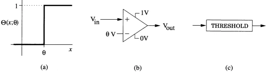
1.1 The threshold function. (a) A graph of the threshold function. (b) The threshold function implemented with a high gain amplifier configured as a comparator. (c) The function block with which the threshold function will be represented in block diagrams.

. . .

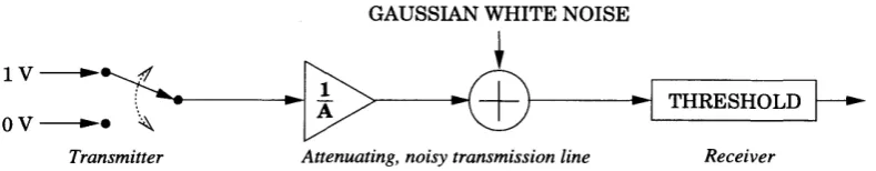
6 1.2 A schematic diagram illustrating the use of a threshold function to suppress

noise introduced by transmitting a signal down an attenuating, noisy trans- mission line.

. . .

7 1.3 A graph of the probability distributions p(Dolz) and p ( D l l z ) .

. . .

7 1.4 The use of threshold functions as repeaters. Attenuation reduces the signal

voltage as it travels down the noisy transmission line, but the repeaters peri- odically reset the voltage to their best estimate of the originally transmitted value. This can be used to limit the error introduced by noise regardless of what distance the signal travels.

. . .

9

2.1 Schematic representations of the receptive fields of two typical simple cells in primary visual cortex. The dark coloration represents the part of the receptive field responsive to illumination which is darker than background, the light coloration represents responsiveness to lighter than background illumination. The receptive field on the left is therefore responsive to a n oriented step change in illumination; the one on the right is responsive to an oriented line. Based on a figure in [Miller, 19951.

. . .

12 2.2 The prototypical statistical signal model. Independent, white, stochastic in-

novations processes drive corresponding innovations filters which are summed together to produce the observed process.

. . .

14 2.3 The standard model. One white, Gaussian innovations process drives the

2.4 The optimal innovations estimator for the standard model. Given the observed process of the standard model, the optimal estimate of the innovations process

. . .

is the linear filter Ho. 17

2.5 An image analyzed in the context of the standard model. Left: A sample real image. Rzght: The image passed through the innovations estimator derived from the average power spectrum of a database of photographs (refer to (2.5)). 17 2.6 The features model. The standard model is augmented with Poisson impulse

innovations processes and their corresponding innovations filters which have impulse responses in the shape of various visual features.

. . .

19 2.7 The observed process of the first stage. A single binary innovations process,

the innovations process of the standard model, and no innovations filters.

. .

20 2.8 The optimal innovations estimator of the first stage. A threshold function.

.

21 2.9 The observed process of the second stage. The binary innovations process il

is passed through an innovations filter GI, then added to the white Gaussian

. . .

innovations process io to produce the observed process. 22 2.10 The optimal innovations estimator of the second stage. The estimator is a

linear matched filter followed by a threshold acting as a nonlinear classifier. 25 2.11 The geometric illustration of the matched filter in two dimensions. The space

shown is the vector space of a two dimensional z[k], so that the abscissa is z[k] and the ordinate is z[k - 11. The circles mark the equiprobability contours at one standard deviation of p(z [k]

I

D o ) and p(z[k]

I

Dl )

.

The vector h l represents the matched filter; applying the filter is equivalent to projecting z onto h l . The dotted line is the graph of p(z[k]

I

D o ) = p(z[k] (D l ) , which also marks the decision plane defined by applying the threshold function to the output of the

. . .

matched filter. 25

. . .

1X

2.13 The geometric illustration of the why the matched filter developed in Sec- tion 2.3.2 does not work when the Gaussian process is correlated (nonwhite). The elipses mark the equiprobability contours at one standard deviation of

p(z[k]lDo) and p(z[k] ID1). The dotted line is the graph of p(z[k] IDo) =

p(z[k]

1

D l )

,

and the dashed line is the decision boundary that would be formed if a matched filter were applied directly; since these two lines do not coincide, the matched filter is not optimal. This situation may be transformed into the one shown below in Figure 2.14 by first passing z through a whitening filter,

. . .

after which a matched filter may be applied. 27

2.14 The geometric illustration of using a matched filter after applying a whitening filter to the situation illustrated in Figure 2.13. After the whitening filter is applied, it is the same geometric scenario shown in Figure 2.11.

. . .

28 2.15 The innovations estimator of the third stage. The generalized matched filter

is a whitening filter followed by a postwhitened matched filter. . . 29 2.16 The observed process of the fourth stage, the complete bandlimited features

model. This is a bandlimited version of Figure 2.6.

. . .

29 2.17 The optimal innovations estimator for the fourth stage, the complete bandlim-

ited features model. The observed process is whitened, then processed by a bank of matched filters. The largest matched filter output is selected by the

WINNER TAKE ALL block and is then passed through a threshold function.

.

32

2.18 The geometric illustration of the optimal innovations estimator for a features model with three feature generators. The axes represent the components of the two dimensional, postwhitened, observed process

ii.

As before, the circles mark the equiprobability contours at one standard deviation of p(E[k] ID,). The dashed lines are the decision boundaries formed by the winner-take-all operation, and the dotted lines are the decision boundary formed by the action

. . .

of the threshold function. 33

2.19 Adding lighting level variation and sensor noise to the model. The sum of the innovations processes passed through their corresponding innovations filters is multiplied by a statistically independent, non-negative gain term representing lighting level variation and is then summed with a white, Gaussian noise

. . .

X

2.20 Countering the effects of lighting level variation by estimating the light level and dividing it out. Sensor noise is smoothed by the filter Q whose spa- tial frequency response is adjusting according to the estimated lighting level (represented by the arrow between the light level estimator and the filter Q ) . 38 2.21 Left: An image from MIT Media Lab face database Right: The normalized,

smoothed and whitened image. Because the post-whitened image has nega- tively valued pixel amplitudes, the luminance values were chosen such that grey represents a pixel amplitude of zero, black represents the most negative amplitude value and white the most positive. This convention is also used in

. . .

the figures below. 40

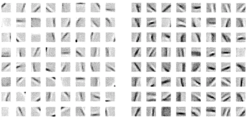
2.22 Left: The receptive fields of 64 simulated simple cells after training on a set of 250 randomly selected images from the MIT face database. Each receptive field has a dimension of 8 x 8 pixels. The images have been smoothed to elim- inate pixelation, and as in Figure 2.21, grey represents zero pixel amplitude. Right: A set of 64 receptive fields which were automatically centered in their pixel blocks during training to avoid translational redundancy.

. . .

41 2.23 Control cases to ensure that the simulated simple cell receptive fields represent

features in the data, not artifacts. Left: Result of training on images whose pixels were randomly scrambled. Right: Result of training on images whose pixels were scrambled, then passed through a

&

filter so that they have the power spectrum of real images. Neither case produced the type of receptive fields shown in Figure 2.22, as would be expected.

. . .

41 2.24 Left: A 128 x 128 section of the IEEE standard image, "Lena," which was not

used in training. Center: Result of reconstructing the image from simulated simple cell responses (see text for explanation). Right: The normalized,

. . .

smoothed and whitened image, shown for comparison. 42

xi

2.26 The subband statistical signal model. The white, Gaussian innovations pro-

cess of the standard model is augmented by a bank of innovations processes which switch between a white Gaussian source and zero driving a bank of innovations filters which divide the spectrum into frequency bands.

. . .

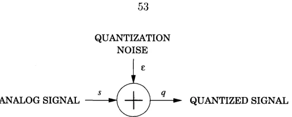
3.1 Block diagram of the amplitude quantizer. A continuously valued signal s

is passed into a quantizer which converts it into a quantized signal q whose amplitudes belong to a countable set of quantized levels.

. . .

3.2 Block diagram of the integrate-and-fire circuit (IFC) used in the context of

neural transmission. The analog valued dendritic current s is transformed by the IFC, a model of somatic spike rate encoding, into the quantized spike train q. The axon carries the spike train q to its destination, the target cell's dendrite, which is modeled as a linear filter H. The filter H has a low pass

. . .

response, which serves to convert q into an estimate of s.

3.3 Left: The output of a n ideal quantizer with step size A of one (solid line), plot- ted with the identity function for comparison (dashed line). Right: A sample waveform s (dashed line) plotted along with its quantized representation q (solid line).

. . .

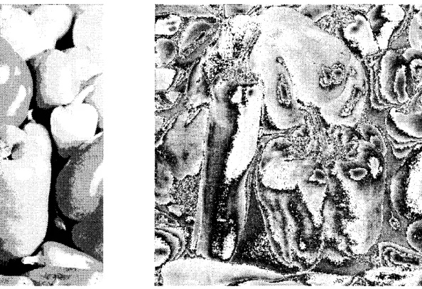
3.4 Left: Various effects of quantization are illustrated below by quantizing the pixel luminance values of an image. Each of the 512 horizontal scan lines of the image will be treated as if it were a one second long, time varying signal and independently quantized. Right: The IEEE standard image "peppers"

. . .

which is the actual image used for the illustrations.

3.5 Block diagram of the equivalent model of quantization as the addition of

quantization noise E .

. . .

3.6 Graph of the value of quantization noise E as a function of quantizer input

. . .

for an ideal uniform quantizer with step size A = 1.

3.7 Left: Result of passing luminance amplitudes of each scan line of the image in Figure 3.4 through a five level uniform quantizer, illustrating the distorting effects of signal-dependent quantization noise E . Right: The quantization noise E itself, obtained by subtracting the original signal s from its quantized

3.8 Block diagram of the noise added prior to quantization. A continuously valued signal s is summed with a zero mean, Gaussian white noise source before being fed into the quantizer. The noise may be artificially added or inherent background noise in a physical system.

. . .

56 3.9 The distribution of quantization error t[k] for a uniform quantizer with step

size A = 1 with three different standard deviations of the additive Gaussian

A A

noise source n: Left: a, = E , Middle: a, = 7 , Right: an =

.

Each graph displays the distributions for three representative values of the signal amplitude s [k]: 0.25 (dash-dotted line), 0.5 (dashed line), and 0.75 (solid line). In the graph on the left, the quantization error is systematically dependent on the signal amplitude, but by the graph on the right, the quantization error is approximately statistically independent of the signal amplitude.

. . .

57 3.10 Left: Result of first adding zero mean, Gaussian white noise n with stan-

dard deviation

-$

before passing the scan lines of the image through a five level uniform quantizer, then subtracting the noise n so that the only noise remaining is signal-independent quantization noise E . Quantization noise in this case is well approximated by the addition of a white noise source uni- formly distributed on the interval

[-

$

,

$).

Right: The quantization noise E itself, obtained by subtracting both signal s and noise n from the quantized imageq . . . 58 3.11 Block diagram of the equivalent model of the combination of the additive

. . . . noise source and quantization as the addition of quantization error e. 59 3.12 Graphs of the mean of quantization error elk] of an ideal uniform quantizer

with step size A = 1 as a function of signal amplitude s[k] for three different

A A A

...

X l l l

3.13 Graphs of the correlation of noise n [ k ] and quantization noise elk] of an ideal uniform quantizer with step size A = 1 as a function of signal amplitude s [ k ] for three different noise levels: Left: on =

&,

Middle: on =

+,

Right: on =

$.

The solid line represents the correlation value, and the dotted line is drawn at 0:. For the graph on the right, the correlation is well approximated

as zero with respect to 0:.

. . .

61

3.14 Left: Result of adding zero mean, Gaussian white noise n with standard deviation

$

before passing the scan lines of the image through a five level uniform quantizer, illustrating the sum of the signal s and quantization error e. While the quantization error has a complicated relationship with the signal,

to second-order it is a statistically independent white noise source. Right: The quantization error itself, obtained by subtracting the signal s from the quantized signal q.

. . .

62 3.15 Left: Result of passing the quantized image from Figure 3.14 through a spa-

tiotemporal linear filter designed assuming both a temporal oversampling ratio and a spatial oversampling ratio of four. This reduces the power of the quantization error in the resulting image by a total factor of sixteen times. Right: Result of passing the quantized image from Figure 3.7 through the

same filter, illustrating that signal-dependent quantization error cannot be significantly reduced with linear filtering. . . 62 3.16 Block diagram of the sigma delta quantizer. A signal s plus additive Gaussian

white noise n is integrated, quantized with an ideal uniform quantizer, then differentiated.

. . .

63 3.17 Block diagram of the equivalent model of the sigma quantizer with the quan-

tizer replaced with an additive quantizer noise source E , just as in Figure 3.5. 63 3.18 An alternative block diagram of the equivalent model shown in Figure 3.17.

3.19 A schematic diagram of the power spectra of the noise n and the differentiated quantization noise i. The white noise has a flat power spectrum, while the upper bound on the quantization noise power spectrum grows as w2.&-. If the signal is bandlimited below the point where the two power spectra cross, the quantization noise (which is the sum of n and

i)

is guaranteed to be less than twice the power of the noise n.

. . .

3.20 Block diagram of the integrate-and-fire circuit.

. . .

3.21 Result of passing each horizontal scan line of the "peppers7' image through an

IFC. The image has virtually no noise, and consequently the IFC encoding generates a high level of signal dependent distortion, seen most evidently in

. . .

the encoded image's vertical banding patterns.

3.22 Left: Result of first adding zero mean, Gaussian white noise n before passing each horizontal scan line of the image from Figure 3.4 through a n IFC using the design rule from the last section. Right: Same as the image on the left, but using less noise. See text for details.

. . .

3.23 Left: Result of temporally integrating each horizontal scan line from the IFC

encoded image on the right in Figure 3.22 with a low pass filter whose cutoff frequency is at the bandwidth of s , thus reducing the power of quantization error. Right: Result of doing the same with the image from Figure 3.21, illustrating that a linear filter provides little reduction for signal dependent

. . .

quantization error.

3.24 R.esult of spatiotemporally integrating the image IFC encoded image on the left in Figure 3.22, exploiting the correlation redundancy of neighboring scan . . . lines to reduce quantization error even further than in Figure 3.23.

3.25 The circuit model of the soma. A variable current source provides the input signal s

+

n. When v reaches the threshold voltage E

+

A, the switch closes momentarily setting v back to E and simultaneously, a delta function spike

. . .

is produced in the output signal q (not shown).

xv

3.27 A graph of spike rate as a function of the level of a constant input. The relevant parameters are A = l , g = 0.2. The solid line shows the true spike rate for a leaky integrator SDM and the dotted line shows the equivalent model approximation. Soon after threshold, the approximation is very accurate. 77 3.28 Top left: Result of using an IFC with a leaky integrator to encode the "pep-

pers" image, which was offset so that all luminance values were above thresh- old, then the same amount of noise was added as for the image on the right in Figure 3.23. The leak parameter g was 0.2, and the signal amplitudes ranged between 0.2A and 0.6A. Top right: Result of passing the same im- age through the leak approximation by subtracting O.lA from the luminance values before passing it through a nonleaky IFC. Note that the two images appear qualitatively similar. Bottom left: The result of subtracting the two top images to quantify their similarity. The difference can be mostly charac- terized as noise, but a faint outline of the peppers is visible, representing the error in the approximation of the equivalent model. The difference is most noticeable at the lowest signal levels (for example, the long pepper on the left is the most visible). Bottom right: The difference passed through the same spatiotemporal integration filter used in Figure 3.24.

.

.

. . . .

.

. . . .

79 3.29 Result of averaging repeated trials of using a leaky IFC to encode a 6Hz

Chapter 1 Introduction

This introductory chapter begins with definitions of the mathematical notation to be used in the course of the thesis. We then present the threshold function, a unifying theme of this thesis, and an example of its use in the detection of digital signals in the presence of noise. This example introduces some of the issues and ideas used in the remaining chapters, whose contents are briefly summarized below:

Chapter 2 describes a model of the development and function of simple cells receptive fields in mammalian primary visual cortex in which a threshold function is used to detect the presence of specific visual features.

Chapter 3 describes a model of neuronal spike rate coding in which a threshold nonlin- earity is used to encode somatic current into a series of axonally transmitted voltage spikes.

Chapter 4 concludes the thesis with a discussion of the common themes of the two models.

1.1

Notation

This section introduces the notational conventions used throughout the remainder of the thesis. Since the primary mathematical concern is the characterization and manipulation of signals, we first define a signal, then present basic analyses to be performed on signals, including Fourier and statistical techniques, and finally introduce linear filtering and vector representations of signals. Futher development of these topics can be found in [Oppenheim et al., 19831, [Papoulis, 19911, [Oppenheim and Schafer, 19891.

1.1.1

Signals defined

A signal is a function of time and/or N-dimensional space. The value of the function is

signal, then s ( x , y) is the signal's amplitude at spatial coordinates (x, y). We use one spatial dimensional signals in derivations for the sake of clarity, but all results can be easily extended to the two-dimensional case.

We will analyze two types of signals, analog and digital, which are classified by their characteristic amplitude values. The amplitude of an analog signal can assume a continuum of values, whereas that of a digital signal can only assume one of a discrete set of values. The most common digital signal is the binary signal, which can only assume one of two amplitude values; unless otherwise specified, all digital signals discussed are assumed to be binary. One of the themes of this thesis is the interconversion between digital and analog signals.

A type of analog signal which arise frequently is the Gaussian process, a signal whose amplitudes are distributed as a Gaussian probability distribution. Another signal which arises in different contexts in the next two chapters is the impulse process, a sum of shifted, non-overlapping Dirac delta functions:

C

6(t - ti), where ti

#

t j if

i

#

j

i

1.1.2

Fourier analysis

A temporal signal x represented as a function of time t can also be represented as a function of frequency in radians per unit of time w by use of the Fourier transform:

where j =

a.

We follow the convention of using capital letters to designate the Fourier transform of a signal. The frequency representation of a signal can be converted back to the time representation with the inverse Fourier transform:

Similarly, a one-dimensional spatial signal s represented as a function of spatial position x can also be represented as a function of spatial frequency w, in radians per unit of space.

A signal s is bandlimited if its Fourier transform is zero for all frequencies w of magnitude

3

signal can be completely represented by amplitude samples spaced T units apart, where T

5

g.

We use the notational convention x[k] to denote these samples, where sample index k is an integer:

A signal of particular interest is the Kronecker delta function, 6[k], which is the bandlimited

analog of the Dirac delta function:

Note that by the definition above, the Kronecker delta function is a binary signal.

1.1.3

Statistical analysis

We will use statistics as a powerful method for characterizing signals and their interrelation- ships. An important statistic is the cross correlation between two signals x and y, denoted

Rxy(7):

where (-) denotes statistical expectation. The function Rxx(t) is known as the autocorrelation of signal x.

If the two signals are bandlimited such that 0,

2

fly, the cross correlation can be represented by samples at intervals of T

<

&:

The Fourier transform of cross correlation is called the cross-power spectrum SXy(w).

00

Sxx(w) =

1

1

R X x ( r ) cos w r d r 0

A white signal has autocorrelation Rxx(t) = 6(t) and power spectrum Sxx(w) = 1. A white bandlimited signal x has an autocorrelation Rxx [k] = 6[k] and a power spectrunl which is constant for frequencies under its bandlimit and zero elsewhere:

(

0 otherwise

1.1.4

Linear filtering

A linear filter performs a particular linear operation which maps signal x to signal y. A linear filter is completely represented by its impulse response, which is itself a signal. If h, is the impulse response of a given filter, the result of applying the filter to the signal x to produce the signal y is computed by an operation known as convolution:

where

"*"

denotes the convolution operator. Convolution of two signals is equivalent to the multiplication of their Fourier transforms:

For sampled signals, convolution is computed by a discrete sum:

A filter of particular interest is the finite impulse response or FIR filter. The impulse

response of an FIR filter is nonzero only in a specific time interval.

1.1.5

Vector representation

This technique allows the application the concepts and methods of linear algebra to signal analysis. We will use boldface type to designate the vector representation of signals.

A bandlimited FIR filter whose impulse response h is nonzero in the range a

<

k

5

b may be entirely represented by the N-dimensional vector h , where N = b - a

+

1. The elements of the vector h are composed of the amplitude samples of the impulse response:

These definitions allow convolution with a bandlimited FIR filter to be expressed as a dot product:

1.2

The threshold function

As mentioned in the beginning of this chapter, the threshold function is a common theme in the models of the next two chapters. In this section, we begin with its definition and a discussion of two of its most important properties, then illustrate its use in the detection of digital signals in noise.

The threshold function O (x; 6 ) outputs a one if its real valued input x is at least as large as the threshold value 6 , zero otherwise.

definitions of the previous section, this function takes an analog amplitude as input and returns a binary amplitude.

Figure 1.1: The threshold function. (a) A graph of the threshold function. (b) The thresh- old function implemented with a high gain amplifier configured as a comparator. (c) The function block with which the threshold function will be represented in block diagrams.

-

Before discussing its application, we highlight its two most important properties: THRESHOLD

The threshold function has only two possible values. The threshold function is non-invertible transformation; in information theoretic terms, 0 ( x ; 0) conveys at most one bit, regardless of how much information was conveyed by z. The threshold function can be used to eliminate information which is irrelevant to a particular task, and for this reason, it is a computationally powerful tool.

The threshold function has a simple electronic implementation. The threshold function can be implemented with a high gain amplifier configured as a comparator, as illustrated in Figure l . l b . The high gain amplifying the differential input signal drives the amplifier's output to one of its two saturating voltages. Although the amplifier gain would have to be infinite to realize the threshold function exactly, it can be made large enough in practical situations to be considered effectively infinite. In the nervous system, the threshold function can be implemented by a particular neuronal ion channel, the voltage sensitive sodium channel. Either implementation is physically compact, making the threshold function an attractive building block when designing computing hardware, whether silicon- or carbon-based.

The threshold function will be represented in block diagrams with the symbol shown in

[image:21.616.105.538.144.262.2]

1.2.1

The detection of digital signals in the presence of noise

One of the primary uses of the threshold function is for the detection of digital signals in the presence of noise, which has application in insuring the accuracy of digital signal transmission along a noisy, attenuating electrical transmission line. This is not only a standard situation in modern electronic communications, but also in the nervous system, as is discussed in Chapter 3. In Chapter 2, we show that it also has application to the detection of visual features in images.

GAUSSIAN WHITE NOISE

I

THRESHOLD -+

0V-• %

Transmitter Attenuating, noisy transmission line Receiver

Figure 1.2: A schematic diagram illustrating the use of a threshold function to suppress noise introduced by transmitting a signal down an attenuating, noisy transmission line.

A schematic diagram of the transmission scenario is shown in Figure 1.2. At any par- ticular time, the amplitude of the transmitter's signal is either one volt or zero volts. As the signal is travels along the transmission line, its power is attenuated and it is corrupted by the electrical noise, resulting in uncertainty at the receiver as to which amplitude was actually transmitted. The goal of the receiver is to estimate, with as little error as possible, which voltage was sent by the transmitter. As will be shown, this can be accomplished with the threshold function.

Figure 1.3: A graph of the probability distributions p(D01.t) and p(Dllz).

[image:22.619.127.522.248.325.2] [image:22.619.138.514.546.664.2]

8

D l denote that a one was transmitted:

We model the attenuation with a gain of

i,

where A is the level of attenuation, and the effects of noise are represented by the addition of a zero mean, Gaussian random variable of variance 02. The probability distributions of the received voltage amplitude z given the two different possibilities, Do and D l , are shown in Figure 1.3:

In order to minimize the error of estimation, the receiver must choose the more likely scenario, Do or D l , given x. If D l is more likely given x, the receiver should assume that a one was transmitted:

Assume s = 1 if p(D1 1x)

>

p(Do ( 2 ) By Bayes' theorem, this is equivalent to

If we assume that one and zero voltage transmissions are equally likely, then p ( D o ) =

p(D1) =

$.

Since the additive Gaussian noise has the same variance for both distributions

p(zlDo) and p(xlD1), (1.22) is equivalent to

Note that the receiver will inevitably make some errors in its estimation of the transmitted signal. Due to the overlap of the two probability distributions p(x

1

D o ) and p(zl D l ), there are two types of errors. An error of type I occurs when values of x due to Do are rnisclassified as signifying a one was sent (this is also known as a false alarm). Similarly, when values of z due to Dl are misclassified as signifying a zero was sent, this is a type I1 error. The total error rate is their sum, and for our classification scheme this is

By performing the classification as described above, this probability was minimized. How- ever, type I and type I1 errors can be weighted asymmetrically if their consequences are not equivalent. In this case, the threshold level may shift from one half to minimize a weighted error probability. This point is discussed in Chapter 2 in the context of feature detection.

NOISE NOISE NOISE

. - - - . - . _THRESHOLD

}---

Figure 1.4: The use of threshold functions as repeaters. Attenuation reduces the signal voltage as it travels down the noisy transmission line, but the repeaters periodically reset the voltage to their best estimate of the originally transmitted value. This can be used to limit the error introduced by noise regardless of what distance the signal travels.

10

given enough repeaters regardless of how far the signal must travel to reach its destination. Repeaters are commonly used in electrical communication, and as is pointed out in Chapter 3, in the axonal transmission lines of the nervous system.

Chapter

2

A

Model of Visual Feature Detection

2.1

Introduction

This chapter describes a model of the development and function of simple cell receptive fields in mammalian primary visual cortex. The model assumes that images are composed of combinations of a limited set of specific visual features and that the goal of simple cells

is to detect the presence or absence of these features. Based on a presumed statistical character of images and their visual features developed below, the model uses a constrained Hebbian learning rule to discover the structure of the features, and thus the appropriate response properties of simple cells, by training on a database of photographs. The response properties of the model simple cells agree qualitatively with neurophysiological observation.

2.1.1

The primary stages of mammalian visual processing

We begin with a brief review of the focus of our modeling efforts: the structure and func- tion of the primary stages of mammalian visual processing (for a complete discussion see [Wandell, 19951). The luminance intensities of an incoming visual image are transduced by the photoreceptor array of the retina. Since the dynamic range of their output is limited, the receptors automatically adjust the scale of their photosensitivity to match the ambient light level. Retinal circuitry then enhances image contrast by computing the differential between each photoreceptor's output and the outputs of its neighbors; this is known as the center-surround organization of the retina. The resulting image is relayed through the tha-

lamus to the visual area of cortex. In the first area of cortical visual processing, labeled V1 in primates, there are a class of cells known as simple cells which respond to certain

Figure 2.1: Schematic representations of the receptive fields of two typical simple cells in primary visual cortex. The dark coloration represents the part of the receptive field responsive to illumination which is darker than background, the light coloration represents responsiveness to lighter than background illumination. The receptive field on the left is therefore responsive to an oriented step change in illumination; the one on the right is responsive to an oriented line. Based on a figure in [Miller, 19951.

The goal of our modeling efforts is to offer an information theoretic argument as to why simple cells are tuned for a specific spatial frequency and orientation and to propose a mechanism for developing their specificities based on sensory experience with the visual world. Much work has already been done on this topic, which will be summarized next, and the final section of this chapter includes a discussion of our model in the context of the literature.

2.1.2

Models of simple cell receptive fields

In the following brief survey of previous modeling of simple cell receptive fields, we divide the models into two categories: phenomenological and functional. A phenomenological model of simple cell receptive fields proposes a mechanism which produces patterns which resemble simple cell receptive fields independent of any functional role; in other words, the model is able to replicate the phenomena without providing a n argument for its purpose. In a functional model of receptive fields, the mechanism for the generation of receptive fields is based on their proposed function. Our model falls into the latter category.

13

tractive weight decay. Analysis of this type of model in [Miller and Mackay, 19941 has shown that the resulting receptive fields arise from modes of the correlation structure of the random input. While such models may provide explanations of prenatal development, their use of random input is unrealistic for animals experiencing a sensory world. Furthermore, development is treated as a separate issue from functional operation.

Of the functional models that have been proposed, the most significant is the recent work of [Olshausen and Field, 19961. These authors propose that the computational purpose of simple cells is to form an efficient linear basis for representing images. Their measure of efficiency is "sparseness," meaning that any particular image should be represented with as few basis coefficients as possible. Their model is trained on a database of real images using various nonlinear measures of sparseness, and the resulting receptive fields qualitatively resemble those of real simple cells. As this model is the most similar in the literature to our own, we return to discuss it further in the final section.

2.1.3

Chapter outline

The remainder of this chapter is divided into six sections. Since the simple cell receptive field model is based on assumptions about the statistical character of images, the first section is both a general introduction to the statistical modeling of images and an exposition of our specific statistical model of images as being composed of visual features. In the second section, we establish the theoretical basis for our model of the function of simple cells by deriving the optimal detection strategy for visual features, assuming their form is known. The section concludes by describing the model in terms of specific neurobiological mechanisms. In the third section, the specific form of the features is assumed to be unknown, and a constrained Hebbian learning rule is derived to determine the form of features from example images. This Hebbian rule serves as our model for the development of simple cell receptive fields. In the fourth section, the model is elaborated to accommodate variation in lighting conditions and sensor noise. The fifth section contains results from training on a database of photographs, and the model simple cell receptive fields are shown to be qualitatively similar to those observed experimentally. The last section discusses the model in terms of its relation to the work of other authors, the mathematical techniques used, and its potential for further application.

14

tioned in that section, all derivations below use one-dimensional spatial signals to simplify notation, but the results naturally generalize to the two dimensions of real images.

2.2

Statistical signal models of images

Perhaps the most powerful and successful technique for describing the highly complex struc- ture of images is to model an image as if it were the output of a stochastically driven process. This section begins with the introduction of the prototypical structure of statistical signal models, followed by two specific models. The first is the standard model, which forms the basis for the methods of classical linear signal processing. After presenting it, we demon- strate its limitations as a model of real images. We then propose a more detailed model of real images, the features model, which will be fully developed in following sections as a basis for explairiing the development and function of simple cell receptive fields.

2.2.1

The prototypical model

The prototypical statistical signal model is that one or more independent, white, stochastic signal sources known as innovations processes are passed through corresponding linear in- novations filters and then summed together to produce the observed process; the observed process is the image seen by the observer. The model is illustrated in schematically in Fig- ure 2.2, and the notational conventions which will be used to describe the various parts of the model are summarized in the table below.

Innovations processes Innovations filters

WHITE STOCHASTIC PROCESS

WHITE STOCHASTIC PROCESS

Observed process Signals

Using this notation, the equations describing the model can be written as follows. Each of the innovations processes im is passed through an innovations filter to generate signal :,s

zm

G m

Sm

S m

x

where

"*"

denotes convolution and x is one-dimensional spatial position. The observations process x is the sum of all of the signals :,s

Innovations process m (a white, stochastic process)

Spatial frequency response of innovations filter m (a linear filter) Impulse response of innovations filter m (a linear filter)

Signal rn (innovations process m passed through innovations filter m )

Observed process (sum of the signals, the image seen by the observer)

For any particular model of this structure, two items must be specified based on our a priori hypotheses about the mechanisms underlying image generation: the number of innovations processes and filters and the stochastic nature of the individual innovations processes. The spatial frequency response or impulse response functions of the innovations filters may then be adjusted so that the model best fits a representative set of real image data.

The innovations processes are the sources of information in the image, and therefore an important statistical signal processing operation is to optimally estimate the innovations processes given the observed process. Optimality is defined in the minimum mean squared error sense,

i.

e. the optimal estimator produces the minimum mean squared error between its estimate of an innovations process and the true innovations process. The optimal inno- vations estimator can be used to perform many fundamental signal processing tasks such as redundancy reduction, noise suppression, and in the context of the proper image model, feature detection.

For each of the two models considered below (the standard model and the features model), we are therefore interested in specifying the following:

16

The stochastic nature of the individual innovations processes.

How to adjust the spatial frequency response or impulse functions of the innovations filters to best fit real image data.

The optimal innovations estimator.

2.2.2

The standard model

The standard model is the simplest possible form of the prototype outlined in the last section. It has one white Gaussian innovations process io with unit variance and a single innovations filter Go, as illustrated in Figure 2.3.

Innovations process Innovations filter

Figure 2.3: The standard model. One white, Gaussian innovations process drives the linear innovations filter Go.

WHITE GAUSSIAN PROCESS

-

As discussed in the previous section, the model must be fit to real image data by adjusting the frequency response of the innovations filter, Go(jwx). The power spectrum of images predicted by the standard model is

-

The innovations filter Go(jw,) can therefore be fit using the estimated power spectrum of real images

sZz

(w,) :

- Go

As has been reported in the literature [Field, 19941, by using a database of photographs to estimate S,,, one finds that Go(jwx) is approximately proportional to

5 .

The final task is to specify the optimal innovations estimator. For the standard model, the estimator is a linear filter, as illustrated in Figure 2.4. The filter has the form

Observed process

Observed process Innovations estimate

e

Figure 2.4: The optimal innovations estimator for the standard model. Given the observed process of the standard model, the optimal estimate of the innovations process is the linear filter Ho.

While the standard image model has been successfully used in many applications, it has a significant limitation: the signals it describes lack the semantic content of real images. We hypothesize that an important aspect of real images is that they contain visual features, which we define with the following:

D E F I N I T I O N A feature i s a specific spatial pattern which can be described as being present

o r absent i n a n y given image location.

By this broad definition, a feature may be something as simple as a line segment or as complex as a human face.

Figure 2.5: An image analyzed in the context of the standard model. Left: A sample real image. Right: The image passed through the innovations estimator derived from the average power spectrum of a database of photographs (refer to (2.5)).

18

more detailed model which supplements the standard model with stochastic processes which explicitly add features.

2.2.3

The features model

Central to the definition of a feature is the idea that a binary judgment can be made about whether it is present or absent at any given image location. The features model therefore augments the standard model with a set of M Poisson impulse innovations processes to generate M distinct visual features. Recalling the definition from Section 1.1.1, an impulse process is the sum of uniquely shifted Dirac delta functions:

i,(x) =

C

b(x - xj), where x j

#

xk if j

#

k _(2.6) j

In a Poisson impulse process, the positions of the impulses are statistically independent. Although in the prototype statistical signal model asserts that the innovations processes be white, we relax this slightly for the Poisson process to allow a nonzero mean. If the mean of a particular Poisson process is A, its power spectrum is white plus a DC term:

When passed through a linear innovations filter Gm, an impulse process produces a series of shifted images of the impulse response of G,:

The feature is thus only present in the image at spatial locations {xj}. In the features model, the impulse responses of the additional innovations filters define the characteristic form of each feature. Referring to the examples of features mentioned in the previous section, the inlpulse response of an individual filter might be as simple as a line segment or as complex as a human face. We denote the combination of an impulse process and its corresponding innovations filter as a feature generator. The more feature generators the model uses, the less necessary the white Gaussian innovations process.

Innovations processes Innovations filters

WHITE GAUSSIAN PROCESS

POISSON IMPULSE PROCESS

POISSON IMPULSE PROCESS

POISSON IMPULSE PROCESS

Figure 2.6: The features model. The standard model is augmented with Poisson impulse in- novations processes and their corresponding innovations filters which have impulse responses in the shape of various visual features.

-

generating that feature. Due to the binary nature of the impulse innovations processes, the optimal estimator involves the use of a nonlinear classifier. It is our hypothesis that the simple cells of visual cortex act as such estimators.

In accordance with our discussion in Section 2.2.1, there are two important aspects to specify in the model. First, in the next section we derive the form of the optimal innovations estimators which serve as feature detectors. Second, in the following section we specify a method for fitting the model's parameters, and thus the parameters of the innovations estimators, to real image data.

2.3

The optimal innovations estimator for the features model

Go

In this section, we derive the optimal innovations estimator for the features model in four stages of increasing complexity. In the first stage, the optimal innovations estimator is derived for a features model reduced to the Gaussian innovations process and a single impulse innovations process with no innovations filters. The second stage adds an innovations filter for the impulse process, the third stage adds the innovation filter for the Gaussian innovations process, and in the fourth stage the estimator is derived for the complete features model. Much of the mathematical development outlined below is well known in detection theory, which is discussed in detail in [McDonough and Whalen, 19951.

One important practical difference between the rnodels discussed in this section and the

Observed process

-

f \

+

J

-

Gl

-

-

-

GM -\

20

features model as originally described is that all signals are assumed to be baridlimited due to physical constraints. The images are therefore represented by discrete samples of their luminance amplitude, known as pixels, and the impulse innovations processes are bandlimited impulse processes composed of shifted Kronecker delta functions:

C

6[k - ki], where ki

#

i$i if i

#

j

i

We make a series of five constraining assumptions about the innovations processes and filters for the purpose of mathematical tractability. The utility of these assumptions is demonstrated in the results section by using the model on real image data.

2.3.1

The first

stage

The first stage of deriving the optimal innovations estimator begins with only one of the bandlimited, binary valued innovations processes, i l , whose two amplitude values are zero and one. The probability of a sample with amplitude one (il [k] = 1) is parameterized by A, and the probability of zero (il[k] = 0) is thus 1 - A. The parameter X must be known a priori. Each sample of il is chosen independently, so that knowledge of il[k] does not bias the probability distribution of il[k

+

11.

The observed signal is the sum of this innovations process and the Gaussian innovations process, io. We assume for now that io has a variance of one, and so each sample of the observed process z is therefore a sum of il[k] and an independently drawn, zero mean, Gaussian random variable io[k] of variance one:

Innovations processes

-

WHITE GAUSSIAN PROCESS

Observed process

1

21

Given z[k], the receiver must estimate il[k] with minimum error. This is the same scenario as the communications problem posed in Section 1.2.1; as before, the threshold function 0 ( x ; 8 ) serves as the optimal estimator. This scenario is diagrammed in Figure 2.7.

Ubserved process Innovations estimate

THRESHOLD

+

Figure 2.8: The optimal innovations estimator of the first stage. A threshold function.

Paralleling the discussion in Section 1.2.1, we denote il[k] = 0 by Do and il[k] = 1 by Dl. The value of 8 should be set so that O (il [k]

+

io [k]; 8 ) will be one when

and zero otherwise. Unlike the derivation in Section 1.2.1 p(D1)

#

p ( D o ) ; in fact, p(D1) = X

and p ( D o ) = 1 - A. The conditional probability distributions for z[k] are therefore

The optimal 8 satisfies the equation

Using Bayes' rule and substituting the Gaussian probability distributions above:

Solving for 8,

2.3.2

The second stage

The next stage of complexity is to pass the innovations process il through the innovations filter G1 to produce s l . Estimating il will therefore involve examining multiple pixels of z. In order to constrain the number of pixels N that must be examined, we constrain G1 to have a finite impulse response, which is the same as constraining visual features to have a finite spatial extent in the image.

A S S U M P T I O N 1 The impulse response of each feature generator is only nonzero for N pixels,

where N is a finite number.

The observed process z of the second stage is the sum of sl and the Gaussian innovations process:

z [ k ] = sl [k]

+

i o [ k ]

where sl is defined in (2.1).

Innovations processes

WHITE GAUSSIAN PROCESS

1

0-

Innovations filter

Figure 2.9: The observed process of the second stage. The binary innovations process il is passed through an innovations filter G I , then added to the white Gaussian innovations process io to produce the observed process.

The optimal innovations estimator has two parts. The first is a linear filter H1 called a matched filter, which maximizes the ratio of its response to the signal s , to its response

which is a filter whose impulse response is the spatial reversal of the impulse response of G1. The derivation for this result can be found in [McDonough and Whalen, 19951. We present a geometric argument, using a vector representation of signals1. Using N-dimensional vectors, where N is chosen to be the length of the impulse response of the filter G I , the vector representation of G1 is

Using this, (2.18) may be rewritten as

~ [ k ] = g i

.

il [ k ]

+

io [ k ] (2.21)

Ignoring for the moment other possible values for il [ k ]

,

the estimator should distinguish the following two cases:

If the estimator can accurately distinguish these two cases, it can estimate the value of

i [ k - N

+

11. Since it must make this estimation based on the observed process z , note that the observed vector in the two cases is

24

where hl is an N-dimensional vector whose elements are the elements of g in reverse order ( h l is the vector representation of the matched filter):

Just as in the previous section, Dl is more likely to have occurred when

Making a Bayesian substitution, the two sides of (2.25) are equal at the classification bound- ary:

Since the probability of d[k - N

+

11 being one is A, p(D1) is also X and p ( D o ) = 1 - A. Furthermore, because io is white, the probability distributions of the two cases are that of uncorrelated, multivariate Gaussian random vectors:

1 -(z[k] - h l )

.

(z[k] - h l )

p(z[kllD1) = 7 exp

(27r) -5 2

Making the appropriate substitutions in (2.26) and solving:

1 1 - X

hl z[k] = -hl

.

hl

+

ln-

2 X

If 8 is set to

which combines passing the observed process through the matched filter (hl

-

z[k]) and the threshold operation. The innovations estimator is illustrated schematically in the block diagram of Figure 2.10 and geometrically in Figure 2.11.

Figure 2.10: The optimal innovations estimator of the second stage. The estimator is a linear match,ed filter followed by a threshold acting as a nonlinear classifier.

Figure 2.11: The geometric illustration of the matched filter in two dimensions. The space shown is the vector space of a two dimensional z[k], so that the abscissa is z[k] and the ordinate is z[k - 11. The circles mark the equiprobability contours at one standard deviation of p(z[k] (Do) and p(z[k]

I

Dl). The vector hl represents the matched filter; applying the filter is equivalent to projecting z onto hl. The dotted line is the graph of p(z[k]

1

Do) = p(z[k]

1

Dl), which also marks the decision plane defined by applying the threshold function to the output of the matched filter.

Observed process

Returning to the earlier caveat of ignoring other values of i[k], there are two cases which are of concern. The first is values of i[k] in which the one value is not the last element of

-

-

the vector. For example,

26

The classifier should assign this to the Do case, since a single feature should not be detected at multiple locations. The second case of concern is more than one occurrence of a feature within a single il[k], which would appear as multiple amplitude one elements. For example,

This case should be classified as D l , since the feature is actually present. In order to simplify these two cases, we make the following assumption:

ASSUMPTION 2 T h e impulse response of each feature generator i s orthogonal t o all spatial

translations of itself of more t h a n K, pixels, where K

<<

N .

By this assumption, the inherent structure of the feature's pattern causes the classifier to act correctly in both situations. If it results in significant misclassifications for shifts of less than K the results of the detector can be averaged and subsampled.

2.3.3

The third stage

The next stage of complexity is to add the innovations filter Go for the white, Gaussian innovations process of the standard model, as illustrated in Figure 2.12. The observed process x of the third stage is the sum of sl and so:

Innovations processes Innovations filters

WHITE GAUSSIAN PROCESS

-

1

- Q

EzT)

Observed p r o c e s ~

0-

The matched filter of the last section is not the optimal estimator for il given this observed process because the samples of so[k] are correlated and the mathematical derivation relied on the assumption of a white Gaussian process. See Figure 2.13 for a geometrical illustration of this point.

Figure 2.13: The geometric illustration of the why the matched filter developed in Sec- tion 2.3.2 does not work when the Gaussian process is correlated (nonwhite). The elipses mark the equiprobability contours at one standard deviation of p ( z [k]

I

D o ) and p ( z [k]

1

Dl ) .

The dotted line is the graph of p(z[k]

1

D o ) = p(z[k]

1

D l ) , and the dashed line is the decision boundary that would be formed if a matched filter were applied directly; since these two lines do not coincide, the matched filter is not optimal. This situation may be transformed into the one shown below in Figure 2.14 by first passing z through a whitening filter, after which a matched filter may be applied.

The optimal estimator for the third stage is the generalized matched filter, which is a linear filter best understood as a combination of two filters: a whitening filter and a matched filter. The whitening filter W is designed to transform the present problem into the matched filter problem by converting the signal so into a white, uncorrelated process. Its form is thus:

We will use the tilde to denote signals after they have passed through the whitening filter. For example, the signal so after it has passed through the whitening filter is go:

28

Also note that the variance of So is now one by definition.

The result of passing the observed process z through the whitening filter is

z [ k ] = So[k]

+

Sl [k]

Since

so

is a white Gaussian process, the matched filter from last section applies. The difference is that the matched filter must now match the impulse response of G1 after passing through W:

Figure 2.14: The geometric illustration of using a matched filter after applying a whitening filter to the situation illustrated in Figure 2.13. After the whitening filter is applied, it is the same geometric scenario shown in Figure 2.11.

This is illustrated geometrically in Figure 2.14. The generalized matched filter is formed from the chaining together of the whitening filter and the matched filter:

The value of 0 is

The complete optimal innovations estimator can therefore be written as

Figure 2.15: The innovations estimator of the third stage. The generalized matched filter is a whitening filter followed by a postwhitened matched filter.

Observed process -- Innovations estimate

2.3.4

The fourth

stage

THRESHOLD

The fourth stage is the complete features model with all innovations processes and their innovations filters. Aside from the white, Gaussian innovations process i o of the standard model, there are M bandlimited Poisson, impulse innovations processes i l . . . ~ , as illustrated in Figure 2.16.

-*

Innovations processes Innovations filters

WHITE GAUSSIAN PROCESS

-

Observed process

*

The observed process of the complete features model is the sum of all innovations pro- cesses passed through their innovations filters:

In order to simplify the design of the optimal innovations estimator, we assume that there is no exact spatial coincidence of features:

ASSUMPTION 3 N o more than one feature is initiated at any given spatial location,.

Mathematically stated, this assumes that at most one of the binary innovations processes has an amplitude of one at any given sample index:

We denote the event that im [ k ] = 0 for all m as Do, and that im [ k ] = 1 as Dm. The probabilities of these events must sum to one:

Based on Assumption 3, the optimal innovations estimator must solve the following equation for m at every pixel:

By making a Bayesian substitution, this is the same as maximizing

In order to solve this equation, the probabilities p ( D m ) of i m [ k ] being one must be specified. In the first three stages, there was only a single necessary a priori parameter A. However,

with M impulse innovations processes, there are potentially M a priori parameters to set. We limit it to a single parameter with the following assumption: