Simplification of Gibbs Free Energy Equation for Predicting the Gas Composition of Steam Gasification of Pattukku Coal Char

Article

Simplification of Gibbs Free Energy Equation for

Predicting the Gas Composition of Steam Gasification

of Pattukku Coal Char

Takdir Syarif

_{, Hary Sulistyo}

_{, Wahyudi Budi Sediawan}

_{, and Budhijanto}

1 Chemical Engineering Department, Faculty of Industrial Technology, Moslem University of Indonesia

Jl. Urip Sumoharjo Km. 05 Makassar, Indonesia

2 Chemical Engineering Department, Engineering Faculty, Gadjah Mada University

Jl. Grafika 2 Yogyakarta 55281, Indonesia

*E-mail: [email protected] (Corresponding author)

Abstract. One of the method to utilize coal as a source of fuel is to convert the coal into a

synthetic gas through the process of gasification. The composition of the gas formed greatly depends on the gasification agent and the process conditions. Currently, some researchers have developed a mathematical model based on thermodynamics to predict the gasification gas composition, based on Gibbs free energy. The equations used to calculate the Gibbs free energy are relatively complex. This study proposes simpler equations to predict the gas compositions in the form of correlation of component’s Gibbs free energy and temperature. The simpler equations proposed were then tested by the experimental data of steam gasification of Pattukku coal char. Base on the result of the experimental and calculation showed if the temperature of gasifier increase by 100 o_{C, the} volume of gas will increase by approximately 1.5 times. The largest average of error obtained for model 1 is 22.95% while from model 2 is 23.45 %. The calculation showed that the proposed model could quantitatively be applied to predict the gas composition of steam gasification of Pattukku coal char.

Keywords: Experimental data, gasification, Gibbs free energy, Pattukku coal char,

thermodynamic model.

ENGINEERING JOURNAL Volume 21 Issue 7

1.

Introduction

Coal is largely available energy source in Indonesia. The deposits can be found in Sumatra, Kalimantan, Sulawesi, and West Papua. Unfortunately, those coals belong to low-grade energy resources (sub-bituminous) [1]. So in order to utilize it, upgrading is needed. One of the methods to upgrade the quality of the coal as an energy source is gasification to produce synthetic gas [2]. Gasification is a thermal process that converts raw materials containing carbon into the flammable gas. In the coal gasification, coal or charcoal was reacted with gasification agents such as oxygen, steam or CO2 [3, 4]. The composition of the formed gas depends greatly on the gasification agent and the operating conditions [5]. When gasification using CO2 is run at a temperature of 900°C, the gas produced will be dominated by the CO and CO2 [6, 7]. Whereas when using the steam, then the most widely produced gas is H2 and CO2.

In the design and operation of the gasification process, the understanding of the influence of raw material and other operating parameters are required. For this reason, mathematical equations or modeling that could be used to perform the optimization of the process is of importance [8, 9, 10, 11]. Some researchers already proposed modeling the process of gasification by using the equilibrium approach. Sharma [12], used thermodynamic modeling and kinetics of the reduction reaction of char in the biomass downdraft gasifier. Zainal et al., [13]; Sharma [14], used the equilibrium model for predicting the distribution of the various types of gas. Florin et al., [15] studied the influence of thermodynamic equilibrium in the formation of hydrogen through gasification of biomass with steam. Jarungthammachote and Dutta [16], developed a thermodynamic equilibrium model based on the equilibrium constants to predict the gas composition in a downdraft gasifier.

In the calculation process, some researchers have used the NASA polynomial equation to the calculation of [17].

(1)

The equation is considered relatively complex because it has seven parameters. Therefore, this study aims to find simpler equations. The study includes laboratory experiments to generate gas composition data of the char gasification process at different temperature and thermodynamics analysis to develop a simple model for predicting the gasification gas composition. The char studied were obtained from Pattukku coal pyrolysis product. In addition, the study also aims to observe the influence of the temperature on the gas volume of gasification products.

2.

Gasification Model

The process of gasification usually performed at high temperatures. So in this study, the reaction is assumed to be spontaneous. According to Bell et al., [6], if the residence time in the gasifier is longer than the reaction time, then the product will be out of a gasifier in a state of equilibrium. Thus, the equilibrium thermodynamic approaches could be used in predicting the gasification gas composition. A nonstoichiometry model is one approach that could be used in the determination of the composition of gasification products when the reaction mechanism is unknown [18, 19]. This model uses a Gibbs free energy minimization approach through Lagrange multiplier and does not require reactions formula in the calculation process.

In the equilibrium, total Gibbs free energy of a system is minimum [20]. Consequently,

(2)

At a certain temperature and pressure, the total Gibbs free energy of a single phase in system with multi-components was defined by [21]:

(3)

T Gg T Fg T Eg T Dg T Cg T Bg Ag T R

G

i i i

i i

i i i o

ln . .

. .

. .

4 3

2   

 

 

0



dG

m

i i

t

i P

T t

n

G

n

G

1

,





_









where are the total Gibbs free energy of a system and ni is mole of each species in the gas product, m is the number of components in the gas product.

The value of is known as the chemical potential μi that can be expressed as :

(4)

Equation (4) can also be expressed in the form of:

(5)

If all the gasses are considered as ideal gasses then fugacity ratio could be replaced by number of mole of the species:

(6)

The combination of Eq. (6) and Eq. (3) results in:

(7)

Equation (7) could be partially differentiated against the number of mole of each species i. It is obtained that:

(8)

In order to get , the value of

(9)

for all i = 1, 2, 3, ...., nm (Eq. (8)). So the minimization of can be conducted by solving simultaneous Eqs. of (9) for all i.

P T t

G

n

G



































f

f

T

R

G

.

.

ln



 o _oi

i i P P T R

G . .ln





































n

n

T

R

G

.

.

ln

3.

Mass Balance

To calculate the number of moles of each component, the constraints of mass balance can be utilized. Based on the concept of mass balance, the mass of each element is conserved. The mass balance of component i can be written as follows:

(10)

4.

Lagrange Multiplier

To solve Eq. (9) using constraint in Eq. (10) the Lagrange Multiplier method is applied. In this method of minimization of Gt with the constraint of Eq. (10) can be done by simultaneously solving Eqs. (9) and (10):

(11)

The solution gives the value of n1, n2,...., nm, 1, 2, ..., k.

The simultaneous equations formed from Eq. (11) in the form of mole fraction (yi) are as follows:





4

0

ln

.

4











_y

T

R

G

_

_

(12a)

 

0

ln

.











_y

T

R

G

_

_

(12b)

 

2

0

ln

.

2









y

T

R

G

_





2

0

ln

.

2











_y

T

R

G

_

_

(12d)





2

0

ln

.

2











y

T

R

G

_

_

(12e)





n a U m i i ij

j . 0, 1,2,3,...

Equation (10) and Eqs. (12a) to (12e) can be solved simultaneously by using Newton-Raphson method.

5.

Model Formulation of

To simultaneously solve Eqs. (10) and (12a) to (12e), the correlation between and temperature (T) are needed. For the purpose, NASA polynomials are available. However, the polynomials are relatively complex. In this study two types of simpler correlations for are proposed, which are as the following:

5.1. Model 1

By definition in the literature [20]:

(13)

By integration Eq. (13), will be retrieved:

(14)

where

(15)

If used the Cpi average, integration of Eq. (15) will be:

(16)

Substitution Eq. (16) into Eq. (14) will be:

(17)

By completing Eq. (17), will be retrieved:

(18)

Furthermore, Eq. (18) can write in the simpler model as follows:

(19)

T

R

G

.



T

R

G

.



T

R

G

.



RT

H

T

RT

G



















 

















T

RT

H

RT

G

RT

G











dT

Cp

H

H





i R i

i H Cp T T

H   

 ,

































T

T

R

Cp

dT

T

R

H

T

Cp

RT

G

RT

G

1

1

2 , ,

























































T

T

R

Cp

T

T

RT

H

T

Cp

RT

H

T

Cp

RT

G

RT

G

R R i R i R R i R i R o R i o

i , , ,

_ln



















T

T

b

a

RT

G

where

5.2. Model 2

Based on the relationship between versus in the literature [11], the equation of as

function of can be expressed in the form:

(20)

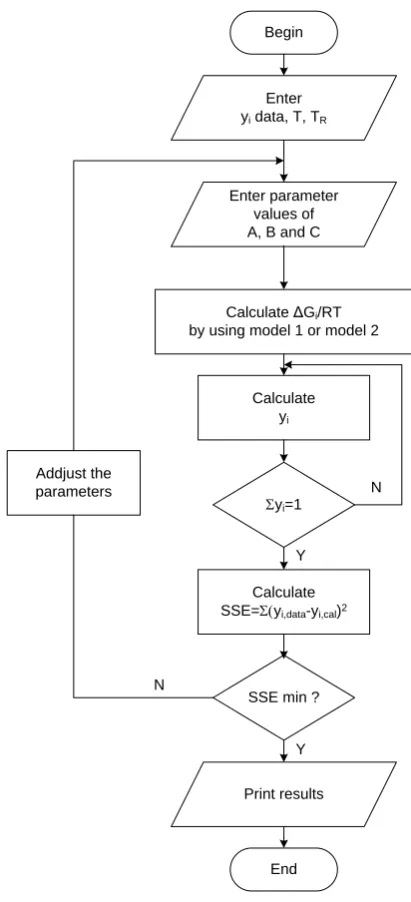
The parameters a1, b1, or a2, b2 in Eqs. (19) and (20) can be obtained by curve fitting in which the value of Sum of Square of Error (SSE):

(21)

is to be minimized. The calculation flow chart is as in Fig. 1.

R R i R i

R o

R i

RT H T Cp RT

G

a₁  ,   ,

R R i

RT

H

b





RT

G



T T_R

RT

G



T TR



















T

T

b

a

RT

G

i

_exp

2 2





















i i data

calculate i

data i

y

y

y

SSE

1

2 _

Fig. 1. Calculation flow chart of the model.

6.

Experimental Setup

6.1. Preparation of Char

The raw material used in the research is char produced by pyrolysis of Pattukku coal obtained

from Lappariaja area, district of Bone South Sulawesi. The pyrolysis was conducted in a quartz

tubular reactor with a diameter of 3.5 cm and a height of 55 cm at 450

_{C and 1 atm. A schematic}

diagram of the pyrolysis equipment is shown in Fig. 2.

One hundred grams of Pattukku coal with a particle size of 3.35-4 mm were fed to the reactor.

Before the process started, nitrogen gas was flowed from the bottom of the reactor to eliminate

the existing air in the reactor. The Pyrolysis was started by switching on the electric furnace to

heating the reactor. The pyrolysis experiment was carried out at fixed temperature (450

_{C) with a}

heating rate of 30

_{C/minutes. After the temperature reached 450}

_{C, the temperature controller}

was turned on and the isothermal process was held for 60 minutes. After that, the reactor was left

Begin

Enter yi data, T, TR

Calculate ΔGi/RT

by using model 1 or model 2

Calculate yi

Syi=1

End

N

Y

Print results Enter parameter

values of A, B and C

Calculate SSE=Syi,data-yi,cal)2

SSE min ? N

Y Addjust the

until the temperature reached 30

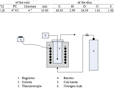
_{C. The elemental composition of proximate and ultimate}

analysis of the coal and the char obtained are presented in Table 1.

Table 1. Proximate and Ultimate analysis results.

Fig. 2. The schematic diagram of the pyrolysis apparatus.

6.2. Gasification Process

The schematic diagram of the gasification equipment is presented in Fig. 3. In the gasification

process, 10 g of char was fed into the gasifier for each experiment. Before the process started,

nitrogen was flowed from the bottom of the reactor to remove oxygen from the reactor. The

experiment was started by switching on the electric furnace to increase the temperature of the

gasifier. After the desired temperature was reached, steam flowed from the bottom of the reactor

at the rate of 5 mL/minute. The non-condensed gas product was collected continuously in a tank

containing water after it passed through the condenser. The volume of the gas collected at the

various time was measured. Gasification process was carried out for 60 minutes, in which every 15

minutes, samples were taken for analysis. The concentration of CH

, CO, H

and CO

were

measured with gas chromatography.

3

4

2 ₅

1

6

Proximate analysis (%) of the coal

VM FC Moisture Ash 38.28 47.92 4.7 10.80

Ultimate analysis (%) of the char

C H O N S

68.93 2.99 24.39 1.81 1.88

Fig

. 3. The schematic diagram of the experimental apparatus.

7.

Result and Disscussion

7.1. Effect of Temperature on the Gas Volume

In this study, the gasification process was run until 60 minutes in a three different temperatures, i.e. 600, 700, and 800 °C. Data obtained include the amount of gas produced and the composition of the four main gasses CH4, CO, H2, and CO2. The volume of gas produced at any time was presented in Fig. 4.

4

8

6

5 ₇

9

10

2 1

11 12

5 ₇

3 ₁₃

14

14

1. Water tank 8. Condenser

2. Pump 9. Condensate tank 3. Nitrogen tank 10. Sampling gas

4. Thermocouple 11. Water tank 5. Coil heater 12. Water reservoir 6. Reactor 13. Steamer

Fig. 4. The relationship between the volume of gas and time at gasification temperature of 600, 700, and 800 °C.

Figure 4 shows the gas volume varies with time at gasification temperature of 600, 700, and 800 °C. It is seen that in general, the volume of gas produced will increase each time and a significant increase occurs until 45 minutes and then the gas volume will be steady.

Furthermore, Fig. 4 also shows that the increase of the temperature results in the increase of the volume of gas produced. The total volume of gas produced at a temperature of 600, 700, and 800 °C is 1701, 2305, and 3483 mL respectively. This significant volume increase shows that the reactor temperature significantly affects the rate of the gasification process. The increase was caused by the reaction between char and steam that are endothermic. So by adding heat into the reactor, the reaction will shift toward products.

7.2. Effect of temperature on the gas composition

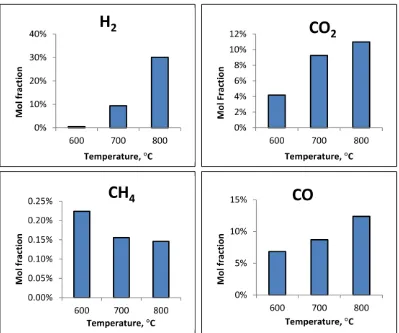
Figures 5 show the effect of the gasifier temperature on the gas compositions. As shown in Fig. 5, the mol fraction of CH4 decreases with the increase of the temperature. At a temperature of 600 °C, mole fraction of CH4 was 0.224% and decreased to 0.156% at a temperature of 700°C. While at a temperature of 800°C mol fraction was 0.146%. It is caused by methanation reaction that is exothermic.

The mole fraction of H2 increases with the increase of the temperature because the reaction between char and steam to produce hydrogen (water gas reaction) is endothermic. So the higher temperature will shift the equilibrium reaction to produce more hydrogen. This indicates that the temperature of the gasifier has an important role in the composition of gas produced by gasification.

From Fig. 5, it seems that the mole fraction of CO increases with the increase of the temperature. At a temperature of 600 °C, mole fraction of CO was 6.83% and increased to 8.7% at a temperature of 700 °C and 12.39% at a temperature of 800 °C. However, the increase of mole fraction of CO from 700 °C to 800 °C was approximately two times larger than the increase of the one from 600 °C to 700 °C. In addition, the increase of mole fraction of CO2 from 700 °C to 800 °C was smaller than the one from 600 °C to 700 °C. Water-gas shift reaction is exothermic thus the reaction equilibrium will shift to produces more CO and less CO2 by increasing temperature.

500 1,000 1,500 2,000 2,500 3,000 3,500 4,000

0 10 20 30 40 50 60

V

olu

m

e

of

gas

, m

L

Time, minutes

Fig. 5. Effect of temperature on the gas composition at 600, 700, and 800 °C for 60 minutes.

7.3. Thermodynamic Analysis

To generalize the experimental result, thermodynamics equilibrium model was applied. Since the temperature was relatively high, the reaction rates were assumed to be fast, so the equilibrium was attained. The gas composition was approximated by thermodynamics equilibrium approach as in Eqs. (10), (12), (13) and (14).

To get the values of the parameters in the equation, curve fitting method was applied. The gas compositions obtained from the calculation were compared to the gas composition from the laboratory experiment. The values of the parameters chosen were the ones that give the minimum value of the sum of squares of errors between the calculated and experimental data (Eq. (16)).

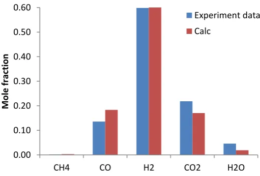
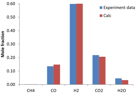
The values of the parameters obtained for model 1 and model 2 are presented in Table 2. Meanwhile, the comparison of calculated results and the experimental values was presented in Figs. 6a-6c and 7a-7c.

Table 2. The parameter values of model 1 and 2.

Component

The equation parameter

Model 1 Model 2

a1 b1 a2 b2

CH4 -17.4685 3.1156 -19.4312 24.001

CO -19.5351 -19.8290 -45.1244 28.4406

H2 10.9054 -5.2005 9.3508 -15.3774

Fig. 6a. Comparison of mole fraction from thermodynamics model and experimental data at gasification temperature 600 °C for model 1.

Fig. 6b. Comparison of mole fraction from thermodynamics model and experimental data at gasification temperature 700 °C for model 1.

Fig. 6c. Comparison of mole fraction from thermodynamics model and experimental data at gasification 0.00

0.10 0.20 0.30 0.40 0.50 0.60

CH4 CO H2 CO2 H2O

M

ole fr

act

ion

Experiment data Calc

0.00 0.05 0.10 0.15 0.20 0.25 0.30 0.35

CH4 CO H2 CO2 H2O

M

o

le

fr

ac

tion

Experiment data

Calc

0.00 0.10 0.20 0.30 0.40 0.50 0.60

CH4 CO H2 CO2 H2O

M

o

le

fr

ac

tion

Figures 6a-6c show a comparison of mole fraction from the experimental result and mole fraction from calculation result by using model 1. It is shown from Figs. 6a-6c that the calculated gas compositions by model 1 and the experimental data were matched with the largest average error was 22.95 % at the temperature of 700 °C while the smallest average of error was 8.09 % at the temperature of 600 °C . Sum of Squares of Errors obtained from the calculation at a temperature of 600, 700, and 800 °C were 0.130, 0.522, and 0.174 respectively.

Figures 7a-7c show a comparison of mole fraction from the experimental result and mole fraction from calculation result by using model 2. It is shown from Figs. 7a-7c that the calculated gas compositions by model 2 and the experimental data were matched with the largest average error was 23.45% at the temperature of 700 °C while the smallest average of error was 8.41% at the temperature of 600 °C. Sum of Squares of Errors obtained from the calculation at a temperature of 600 °C , 700 °C, and 800 °C were 0.118; 0.569 dan 0.213 respectively.

Fig. 7a. Comparison of mole fraction from thermodynamics model and experimental data at gasification temperature 600 °C for model 2.

Fig. 7b. Comparison of mole fraction from thermodynamics model and experimental data at gasification temperature 700 °C for model 2.

0.00 0.10 0.20 0.30 0.40 0.50 0.60

CH4 CO H2 CO2 H2O

M

o

le

fr

ac

tion

Experiment data

Calc

0.00 0.05 0.10 0.15 0.20 0.25 0.30 0.35

CH4 CO H2 CO2 H2O

M

o

le

fr

ac

tion

Experiment data

Fig. 7c. Comparison of mole fraction from thermodynamics model and experimental data at gasification temperature 800 °C for model 2.

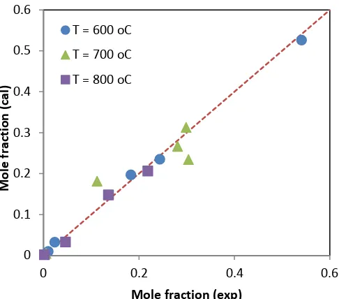
The deviations of the results of model 1 and model 2 to experimental data for all components and temperatures are presented in Figs. 8 and 9. It can be visually observed that the models 1 and 2 were matched to experimental data.

Fig. 8. The deviation of model 1 results to experimental data for all temperatures and gas components. 0.00

0.10 0.20 0.30 0.40 0.50 0.60

CH4 CO H2 CO2 H2O

M

o

le

fr

ac

tion

Experiment data

Calc

0 0.1 0.2 0.3 0.4 0.5 0.6

0 0.2 0.4 0.6

M

o

le

fr

ac

tion

(

cal

)

Fig. 9. The deviation of model 2 results to experimental data for all temperatures and gas components.

By comparing the values of the average of errors and Sum of Squares of Errors of model 1 and 2, it can be concluded that model 1 gives slightly better results than model 2. Since the complexity of model 1 and model 2 are comparable, it is suggested the use of model 1. So, for practicality model 1 is suggested to be applied.

8.

Conclusions

Based on the results of the calculation and experimental data, some conclusions could be obtained as follows:

a. Rising temperatures will increase the volume of gas product. The volume of gas will increase by approximately 1.5 times if the temperature of gasifier increases by 100 °C.

b. Gibbs free energy models proposed could be used to predict the composition of gas produced from char gasification.

c. Although an average of error and SSE value for model 2 is greater than the one of model 1, model 2 is simpler than model 1.

Acknowledgement

The authors would like to thank Ministry of Research, Technology, and Higher Education, Republic of Indonesia for funding this research through BPPDN scholarship

Nomenclature



Agi - Ggi constants in Eq. (1)

µi chemical potential species i (J/mol) Pi partial pressure species i (atm) Po _{total pressure species i (atm)} Uj number of mole element j

aij number of atom element j in species i ni mole species i (mol)

yi mole fraction species i

j Lagrange constants for element j a1 – b1 constants in Eq. (14)

0 0.1 0.2 0.3 0.4 0.5 0.6

0 0.2 0.4 0.6

M

o

le

fr

ac

tion

(

cal

)

Mole fraction (exp)

T = 600 oC

T = 700 oC

a2 – b2 constants in Eq. (15)

References

[1] Kementerian ESDM, “Indonesia: Mineral and Coal Information 2015,” Directorate General of Mining and Coal, p. 37, 2015.

[2] P. Basu, Biomass Gasification and Pyrolysis. US: Elsevier, 2010.

[3] R. Luque and J. G. Speight, Gasification for Synthetic Fuel Production: Fundamentals, Processes and Applications. Elsevier, 2014.

[4] M. Rashid Khan, Advances in Clean Hydrocarbon Fuel Processing: Science and Technology. Woodhead Publishing Series in Energy, 2011.

[5] J. Rezaiyan and N. P. Cheremisinoff, Gasification Technologies, 1st ed. Francis: CRC Press, 2005.

[6] D. A. Bell, B. F. Towler, and M. Fan, Coal Gasification and Its Applications, 1st ed, vol. 1. Elsevier, 2011. [7] S. Lin, M. Harada, Y. Suzuki, and H. Hatano, “Hydrogen production from coal by separating carbon

dioxide during gasification,” Fuel, vol. 81, no. 16, pp. 2079–2085, 2002.

[8] M. Materazzi, P. Lettieri, L. Mazzei, R. Taylor, and C. Chapman, “Thermodynamic modelling and evaluation of a two-stage thermal process for waste gasification,” Fuel, vol. 108, pp. 356–369, 2013. [9] P. Pintana and N. Tippayawong, “Predicting ash deposit tendency in thermal utilization of biomass,”

Engineering Journal, vol. 20, no. 5, pp. 15–24, 2016.

[10] C. Tangsathitkulchai, S. Junpirom, and J. Katesa, “Comparison of kinetic models for CO2 gasification of coconut-shell chars: Carbonization temperature effects on char reactivity and porous properties of produced activated carbons,” Engingeering Journal, vol. 17, no. 1, pp. 13–28, 2016.

[11] A. Farooq, M. Ghauri, and K. Shahzad, “Modeling of biomass gasification with CO2 as gasifying agent,” Sci. Int., vol. 25, no. 3, pp. 497–500, 2013.

[12] A. K. Sharma, “Equilibrium and kinetic modeling of char reduction reactions in a downdraft biomass gasifier: A comparison,” Sol. Energy, vol. 82, no. 10, pp. 918–928, 2008.

[13] Z. A. Zainal, R. Ali, C. H. Lean, and K. N. Seetharamu, “Prediction of performance of a downdraft gasifier using equilibrium modeling for different biomass materials,” Energy Convers. Manag., vol. 42, no. 12, pp. 1499–1515, 2001.

[14] A. K. Sharma, “Equilibrium modeling of global reduction reactions for a downdraft ( biomass ) gasifier,” Energy Conversion and Management, vol. 49, no. 4, pp. 832–842, 2008.

[15] N. H. Florin and A. T. Harris, “Hydrogen production from biomass coupled with carbon dioxide capture: The implications of thermodynamic equilibrium,” Energy, vol. 32, no. 17, pp. 4119–4134, 2007.

[16] S. Jarungthammachote and A. Ã. Dutta, “Thermodynamic equilibrium model and second law analysis of a downdraft waste gasifier,” Energy, vol. 32, no. 9, pp. 1660–1669, 2007.

[17] S. R. Turns, An Introduction to Combustion, 2nd ed. McGraw-Hill, 2000.

[18] B. Acharya, A. Dutta, and P. Basu, “An investigation into steam gasification of biomass for hydrogen enriched gas production in presence of CaO,” Int. J. Hydrogen Energy, vol. 35, no. 4, pp. 1582–1589, 2010.

[19] Q. Yan, L. Guo, and Y. Lu, “Thermodynamic analysis of hydrogen production from biomass gasification in supercritical water,” Energy Convers. Manag., vol. 47, pp. 1515–1528, 2006.

[20] J. M. Smith, H. C. Van Ness, and M. M. Abbott, Introduction to Chemical Engineering Thermodynamics, 7th ed. McGraw-Hill, 2005.

[21] M. J. Moran, H. N. Shapiro, D. D. Boettner, and M. B. Bailey, Fundamentals of Engineering