Nucleon electromagnetic form factors on the lattice and in chiral effective field theory

Nucleon electromagnetic form factors on the lattice and in chiral effective field theory

(QCDSF collaboration)

1_{Institut fu¨r Theoretische Physik, Universita¨t Leipzig, D-04109 Leipzig, Germany} 2_{Institut fu¨r Theoretische Physik, Universita¨t Regensburg, D-93040 Regensburg, Germany} 3_{Physik-Department, Theoretische Physik, Technische Universita¨t Mu¨nchen, D-85747 Garching, Germany}

4_{School of Physics, University of Edinburgh, Edinburgh EH9 3JZ, UK}

5_{John von Neumann-Institut fu¨r Computing NIC, Deutsches Elektronen-Synchrotron DESY, D-15738 Zeuthen, Germany} 6_{Theoretical Physics Division, Department of Mathematical Sciences, University of Liverpool, Liverpool L69 3BX, UK}

7_{Deutsches Elektronen-Synchrotron DESY, D-22603 Hamburg, Germany}

(Received 26 August 2003; revised manuscript received 2 February 2005; published 23 February 2005)

We compute the electromagnetic form factors of the nucleon in quenched lattice QCD, using non-perturbatively improved Wilson fermions, and compare the results with phenomenology and chiral effective field theory.

DOI: 10.1103/PhysRevD.71.034508 PACS numbers: 11.15.Ha, 12.38.Gc, 13.40.Gp

I. INTRODUCTION

The measurements of the electromagnetic form factors of the proton and the neutron gave the first hints at an internal structure of the nucleon, and a theory of the nucleon cannot be considered satisfactory if it is not able to reproduce the form factor data. For a long time, the overall trend of the experimental results for small and moderate values of the momentum transfer q2 _{could be} described reasonably well by phenomenological (dipole) fits

Gpeq2

Gpmq2

p

Gnmq2

n 1q

2_=m2 D

2_;

Gneq2 0

(1)

withmD0:84 GeVand the magnetic moments

p_{2:79 ;} n _{1:91 (2)} in units of nuclear magnetons. Recently, the form factors of the nucleon have been studied experimentally with high precision and deviations from this uniform dipole form have been observed, both at very smallq2 [1] and in the region above1 GeV2 [2,3].

It is therefore of great interest to derive the nucleon form factors from QCD. Since form factors are typical low-energy quantities, perturbation theory in terms of quarks and gluons is useless for this purpose and a nonperturbative method is needed. If one wants to avoid additional assump-tions or models, one is essentially restricted to lattice QCD and Monte Carlo simulations. In view of the importance of nucleon form factors and the amount of experimental data available, it is surprising that there are only a few lattice investigations of form factors in the last years [4,5].

In this paper we give a detailed account of our results for the nucleon form factors obtained in quenched Monte

Carlo simulations with nonperturbatively Oa-improved Wilson fermions. We shall pay particular attention to the chiral extrapolation and compare with formulas from chiral effective field theory previously used for studies of the magnetic moments. The plan of the paper is as follows. After a few general definitions and remarks in the next section we describe the lattice technology that we used in Sec. III. After commenting on our earlier attempts to perform a chiral extrapolation in Sec. IV, we investigate the quark-mass dependence of the form factors in more detail on a phenomenological basis in Sec. V. We find that our data are in qualitative agreement with the recently observed deviations [2,3] from the uniform dipole parame-trization of the proton form factors. In Sec. VI we collect and discuss formulas from chiral effective field theory, which are confronted with our Monte Carlo results in Sec. VII. Our conclusions are presented in Sec. VIII. The Appendixes contain a short discussion of the pion mass dependence of the nucleon mass as well as tables of the form factors and of the corresponding dipole fits.

II. GENERALITIES

Experimentally, the nucleon form factors are measured via electron scattering. Because the fine structure constant is so small, it is justified to describe this process in terms of one-photon exchange. So the scattering amplitude is given by

Tfie2uek0e; s0eueke; se

1 q2hp

0

; s0jJjp; si (3)

with the electromagnetic current

J 2

3u

_u1

3

d_{d : (4)}

momenta, ands,s0,. . .are the corresponding spin vectors. The momentum transfer is defined asqp0p. With the help of the form factors F₁q2 _{and F}

2q2 the nucleon matrix element can be decomposed as

hp0; s0jJ_{jp; si up}0_{; s}0

F1q2

i q

2MN

F2q2

up; s (5)

whereMNis the mass of the nucleon. From the kinematics of the scattering process, it can easily be seen thatq2_<0. In the following, we shall often use the new variableQ2 q2_{. We haveF}

10 1(in the proton) asJis a conserved current, while F20 measures the anomalous magnetic moment in nuclear magnetons. For a classical point parti-cle, both form factors are independent ofq2, so deviations from this behavior tell us something about the extended nature of the nucleon. In electron scattering,F₁andF₂are usually rewritten in terms of the electric and magnetic Sachs form factors

Geq2 F1q2

q2 2MN2

F2q2;

G_mq2 _F

1q2 F2q2;

(6)

as then the (unpolarized) cross section becomes a linear combination of squares of the form factors.

Throughout the whole paper we assume flavor SU2 symmetry. Hence we can decompose the form factors into isovector and isoscalar components. In terms of the proton and neutron form factors the isovector form factors are

given by

Gv

eq2 G p

eq2 Gneq2;

Gv

mq2 G p

mq2 Gnmq2

(7)

such that

Gv

m0 Gpm0 Gnm0 pnv1v (8)

with v ₍

v) being the isovector (anomalous) magnetic moment 4:713:71. In the actual simulations we do not work directly with these definitions when we calculate the isovector form factors. We use the relation

hprotonj

₂

3u

_u1

3 d_d

jprotoni

hneutronj

₂

3u

_u1

3d

_djneutroni

hprotonju u_{d djprotoni (9)}

and compute the isovector form factors from proton matrix elements of the current u _{ud dinstead of} evaluat-ing the proton and neutron matrix elements of the electro-magnetic current separately and then taking the difference. Similarly one could use the isoscalar current u _u

dd for the computation of isoscalar form factors, but we have not done so, since in the isoscalar sector there are considerable uncertainties anyway due to the neglected quarkline disconnected contributions.

TABLE I. Simulation parameters, numbers of gauge field configurations used (# configs.) and masses.

cSW cV Volume # configs. am% aMN

6.0 1.769 0.1320 0:331 163_{32 O450 0.5412(9) 0.9735(40)} 6.0 1.769 0.1324 0:331 163_{32 O550 0.5042(7) 0.9353(25)} 6.0 1.769 0.1333 0:331 163_{32 O550 0.4122(9) 0.8241(34)} 6.0 1.769 0.1338 0:331 163_{32 O500 0.3549(12) 0.7400(85)} 6.0 1.769 0.1342 0:331 163_{32 O700 0.3012(10) 0.7096(48)}

6.0 1.769 c0:1353 0.5119(67)

6.2 1.614 0.1333 0:169 243_{48 O300 0.4136(6) 0.7374(21)} 6.2 1.614 0.1339 0:169 243_{48 O300 0.3565(8) 0.6655(28)} 6.2 1.614 0.1344 0:169 243_{48 O300 0.3034(6) 0.5963(29)} 6.2 1.614 0.1349 0:169 243_{48 O500 0.2431(7) 0.5241(39)}

6.2 1.614 c0:1359 0.3695(36)

6.4 1.526 0.1338 0:115 323_{48 O200 0.3213(8) 0.5718(28)} 6.4 1.526 0.1342 0:115 323_{48 O100 0.2836(9) 0.5266(31)} 6.4 1.526 0.1346 0:115 323_{48 O200 0.2402(8) 0.4680(37)} 6.4 1.526 0.1350 0:115 323_{48 O300 0.1933(7) 0.4156(34)} 6.4 1.526 0.1353 0:115 32364 O300 0.1507(8) 0.3580(47)

III. LATTICE TECHNOLOGY

Using the standard Wilson gauge field action we have performed quenched simulations with Oa-improved Wilson fermions (clover fermions). For the coefficient

c_SW of the Sheikholeslami-Wohlert clover term we chose a nonperturbatively determined value calculated from the interpolation formula given in Ref. [6]. The couplings

6=g2 _andc

SW, the lattice sizes and statistics, the values of the hopping parameter (not to be confused with an anomalous magnetic moment) and the corresponding pion and nucleon masses (in lattice units) are collected in Table I. As we are going to investigate nucleon properties, we want to determine the lattice spacing from the (chirally extrapolated) nucleon mass in order to ensure that the nucleon mass takes the correct value. (At the present level of accuracy, the difference between the nucleon mass in the chiral limit and the physical nucleon mass can be ne-glected.) Ideally we would use a formula from chiral perturbation theory for this purpose, e.g., Eq. (A1). Since there seems to be little difference between quenched and unquenched results at presently accessible quark masses it would make sense to apply this formula to our data. However, it turns out that it breaks down for pion masses above 600 MeV [7], where almost all of our results lie (see Fig. 1). (For a detailed discussion of a different approach see Ref. [8].) Hence we resort to a simple-minded phe-nomenological procedure extrapolating our masses by means of the ansatz

aM_N2 _aM0

N2b2am%2b3am%3 (10)

for each . This ansatz provides a very good description of the data [9]. The nucleon masses extrapolated to the critical hopping parameter_c in this way (on the basis of a larger set of nucleon masses) are also given in Table I. Whenever we give numbers in physical units the scale has been set by these chirally extrapolated nucleon masses.

In the last years it has become more popular to set the scale with the help of the force parameter r0 [10]. While this choice avoids the problems related to the chiral ex-trapolation of the nucleon mass, it has the disadvantage that the physical value of r0 is less precisely determined than the physical nucleon mass. Furthermore, as the present paper deals exclusively with nucleon properties it seemed to us more important to have the correct value in physical units for the mass of the particle studied when evaluating other dimensionful quantities like, e.g., radii. It is however interesting to note that the dimensionless prod-uctr₀M0

N is to a good accuracy independent of the lattice spacing. Indeed, takingr0 from Ref. [11] and multiplying by the chirally extrapolated nucleon masses given in Table I one finds r0M0N2:75, 2:72, and 2:73 for

6:0,6:2, and6:4, respectively. Thus the scaling behavior of our results is practically the same for both choices of the scale.

In Fig. 1 we plotM2_N versusm2% using the masses from Table I. The picture demonstrates that scaling violations in the masses are small. Moreover, we see that for m%<

600 MeV our extrapolation curve is quite close to the

chiral perturbation theory curve (A1).

In order to compute nucleon masses or matrix elements we need suitable interpolating fields. For a proton with spatial momentum p~ the most obvious choice in terms of the quark fieldsuxanddxis

B,t; ~p

X

x;x4t

eip~x~.ijkui,xu j

xC5 dkx;

B_,t; ~p X

x;x4t

eip~x~_.

ijkdixC5 u j

xuk,x

(11)

with the charge conjugation matrix C(,, ,are Dirac indices,i,j,kare color indices). Note that we now switch from Minkowski space to Euclidean space.

In Eq. (11) all three quarks sit at the same point. Clearly, as protons are not point objects this is not the best thing to do, and with the above interpolating fields we run the risk that the amplitudes of one-proton states in correlation functions might be very small making the extraction of masses and matrix elements rather unreliable. Therefore

TABLE II. Smearing parameters for Jacobi smearing.

Nsmear smear rrms

6.0 50 0.21 3:5a0:38fm

6.2 100 0.21 5:6a0:44fm

6.4 150 0.21 6:7a0:40fm

0.0 0.2 0.4 0.6 0.8 1.0 1.2 1.4

m2[GeV2]

0.0 0.5 1.0 1.5 2.0 2.5 3.0 3.5 4.0

MN 2 [GeV 2 ]

=6.40 =6.20 =6.00

FIG. 1. Nucleon mass squared versus pion mass squared from the data in Table I. The dotted curve shows our phenomenologi-cal chiral extrapolation (Eq. (10)) for 6:4. The full curve corresponds to the chiral extrapolation derived from chiral perturbation theory (Eq. (A1)) with the parameters given in Appendix A.

we employ two types of improvement: First we smear the sources and the sinks for the quarks in their time slices, secondly we apply a ‘‘nonrelativistic’’ projection.

Our smearing algorithm (Jacobi smearing) is described in Ref. [12]. The parameters N_smear, _smear used in the actual computations and the resulting smearing radii are given in Table II. A typical rms nucleon radius is about 0.8 fm, our smearing radii are about half that size.

The nonrelativistic projection means that we replace each spinor by

! NR1

214 ; !

NR 1

214: (12)

This replacement leaves quantum numbers unchanged, but we would expect it to improve the overlap with baryons. Practically this means that for each baryon propagator we consider only the first two Dirac components. So we only have23inversions to perform rather than the usual4

3inversions— a saving of50%in computer time.

The nonforward matrix elements required for the form factors are computed from ratios of three-point functions to two-point functions. The two-point function is defined as

C2t; ~p

X

,

,hB,t; ~pB 0; ~pi (13)

with the spin projection matrix

1

214: (14)

In the three-point function

C₃t; 3; ~p; ~p0 X

,

_,hB_,t; ~pO3_{B 0; ~p}0_{i (15)}

we have used, besides the matrix (14) corresponding to unpolarized matrix elements, also

1

214i52 (16)

corresponding to polarization in the 2-direction. We then computed the ratios

Rt; 3; ~p; ~p0 C3t; 3; ~p; ~p

0

C2t; ~p

_C

23; ~pC2t; ~pC2t3; ~p0

C23; ~p0C2t; ~p0C2t3; ~p

1=2

:

(17) If all time differences are sufficiently large, i.e., if 0

3t,Ris proportional to the (polarized or unpolarized) proton matrix element of the operator O with a known kinematical coefficient presented below.

For the electromagnetic form factors the operator to be studied is the vector current. In contrast to previous inves-tigations [4,5], which used the conserved vector current, we chose to work with the local vector current

_x

x. The local vector current has to be renormal-ized, because it is not conserved. It should also be im-proved so that its matrix elements have discretization errors ofOa2_{only, which means that we use the operator}

VZV1bVamq icVa@6 6 ; (18)

wherem_q is the bare quark-mass:

amq

1

2

1

2_c: (19)

We have takenZ_Vandb_V from the parametrizations given by the ALPHA collaboration [13] (see also Ref. [14]). The improvement coefficientcV has also been computed non-perturbatively [15]. The results can be represented by the expression [9]

c_V 0:012254

3g

210:3113g 2

10:9660g2; (20)

from which we have calculatedc_V(see Table I). In the limit

g2 _{!0it agrees with perturbation theory [16]. Computing} all these additional contributions in our simulations, we found the improvement terms to be numerically small. Note that the improvement coefficient cCVC for the con-served vector current is only known to tree level so that a fully nonperturbative analysis would not be possible had we used the conserved vector current.

In order to describe the relation between the ratios we computed and the form factors let us call the ratioRfor the

-component of the renormalized vector current more preciselyR. Furthermore we distinguish the unpolarized case (spin projection matrix (14)) from the polarized case (spin projection matrix (16)) by a superscript. The (Minkowski) momentum transfer is given by

q2 _Q2 _2M2

Np~p~0ENp~ENp~0 (21) with the nucleon energy

ENp~

M2

Np~2

q

: (22)

Using the abbreviation

Ap; ~~ p01 _Q2_4M2 N

E_Np~M_NE_Np~E_Np~0M_NE_Np~0

q

we have

Runpol₄ t; 3; ~p; ~p0 Ap; ~~ p0fG_eQ2_M

NENp~ ENp~0

~

p0p~ MNENp~

MNENp~0 GmQ2

~

p0p~2_p~2_p~02_{g; (24)}

Rpol₄ t; 3; ~p; ~p0 Ap; ~~ p0ip0₁p3p03p1

fGeQ2MNENp~ ENp~0 GmQ2p~0p~ MNENp~

M_NE_Np~0g; (25)

and forj1;2;3

Runpol_j t; 3; ~p; ~p0 Ap; ~~ p0iGeQ2MNpjp0j

MNENp~MNENp~0

p~0p~ GmQ2pjENp~p~02 E_Np~0p~0p~ p0_jE_Np~0p~2 E_Np~p~0p~; (26)

Rpol_j t; 3; ~p; ~p0 Ap; ~~ p0

(

GeQ2MNpjp0jp 0 1p3

p0₃p1 GmQ2MNp2p02

~

p0p~_j M_NE_Np~

MNENp~0 p~0p~

X

3

k1

.j2kp0kENp~ pkENp~0

) :(27)

Analogous expressions for the computation of the form factorsF₁ andF₂are obtained by inserting the definitions (6) in the above equations.

We have computed the ratiosRin (17) for two choices of the momentump~,

L 2%p~

0 @00

0 1 A;

0 @10

0 1

A; (28)

and eight choices of the vectorq~p~0p~,

L 2%q~

0 @00

0 1 A;

0 @01

0 1 A;

0 @02

0 1 A;

0 @01

0 1 A;

0 @02

0 1 A;

0 @11

0 1 A;

0 @11

1 1 A;

0 @ 00

1 1

A; (29)

whereLdenotes the spatial extent of the lattice. In Fig. 2 we show two examples of these ratios plotted versus3(for the unimproved operator). The final results forRhave been determined by a fit with a constant in a suitable3interval.

The corresponding errors have been computed by a jack-knife procedure. The values chosen for t and for the fit intervals are collected in Table III.

Generically, several combinations of the above momenta lead to the sameQ2_{, and several ratiosRcontain the form} factors at thisQ2_{with nonvanishing coefficients. Hence we} determined GeQ2 and GmQ2 from an (uncorrelated) MINUIT fit of all theseRs with the corresponding expres-sions (24)–(27) omitting all data points where the error for

R was larger than 25%. The results are collected in the tables in Appendix B. A missing entry indicates a case where the corresponding form factor could not be ex-tracted, e.g., because we did not have sufficiently many

Rs with less than25%error.

The nucleon masses used can be found in Table I. The corresponding errors were, however, not taken into account when computing the errors of the form factors. Varying the

TABLE III. Sink positionstand fit intervals (in3) used for the extraction of the ratiosR.

t Fit interval

6.0 13 [4,9]

6.2 17 [6,11]

6.4 23 [7,16]

0 5 10 15 20

τ

−0.4 −0.2 0.0 0.2 0.4 0.6

0 5 10 15 20

τ

FIG. 2. The ratiosRpol₃ (left) andRunpol₄ (right) plotted versus3 for 6:2, 0:1344. Here p~ ₀~ _{and q~ is the fourth} momentum in the list (29). The vertical dashed lines indicate the fit range for the extraction of the plateau value.

nucleon masses within 1 standard deviation changed the form factors only by fractions of the quoted statistical error.

In general, the nucleon three-point functions consist of a quarkline connected contribution and a quarkline discon-nected piece. Unfortunately, the quarkline discondiscon-nected piece is very hard to compute (for some recent attempts see Refs. [17–19]). Therefore it is usually neglected, lead-ing to one more source of systematic uncertainty. However, in the case of exact isospin invariance the disconnected contribution drops out in nonsinglet quantities like the isovector form factors. That is why the isovector form factors are our favorite observables. Nevertheless, we have also computed the proton form factors separately ignoring the disconnected contributions. The results are given in Appendix B. Regrettably, meaningful values of the electric form factor of the neutron could not be extracted from our data (for a more successful attempt see Ref. [20]). The results for the neutron magnetic form factor are also collected in Appendix B. Note that the isovector form factors have been computed directly (cf. Equation (9)) and not as the difference of the proton and neutron form factors.

IV. CHIRAL EXTRAPOLATION: A FIRST ATTEMPT

The quark masses in our simulations are considerably larger than in reality leading to pion masses above 500 MeV. Hence we cannot compare our results with experimental data without performing a chiral extrapola-tion. In a first analysis of the proton results (see Refs. [21,22]) we assumed a linear quark-mass dependence of the form factors. More precisely, we proceeded as follows.

Schematically, the relation between a ratio R (three-point function/two-(three-point function) and the form factors

Ge,Gm can be written in the form

R hp0jJjpi ceGecmGm (30)

with known coefficientsce,cmfor each data point charac-terized by the momenta, the quark mass, the spin projection and the space-time component of the current. Assuming a linear quark-mass dependence ofGeandGmwe performed a 4-parameter fit,

Rc_ea_eam_q c_eb_ec_ma_mam_q c_mb_m; (31)

of all ratiosR belonging to the same value ofQ2 _{in the} chiral limit. The resulting form factors in the chiral limit are typically larger than the experimental data. They can be fitted with a dipole form, but the masses from these fits are considerably larger than their phenomenological counter-parts [21,22].

What could be the reason for this discrepancy? Several possibilities suggest themselves: finite-size effects, quenching errors, cut-off effects or uncertainties in the chiral extrapolation. The length Lof the spatial boxes in our simulations is such that the inequalitym_%L >4holds in all cases. Previous experience suggests that in the quenched approximation this is sufficient to exclude con-siderable distortions of the results due to the finite volume. This assumption is confirmed by simulations with Wilson fermions, where we have data on different volumes. Quenching errors are much more difficult to control. However, first simulations with dynamical fermions indi-cate that — for the rather heavy quarks we can deal with — the form factors do not change very much upon unquench-ing [22]. Havunquench-ing Monte Carlo data for three different lattice spacings (see Table I) we can test for cut-off effects in the chirally extrapolated form factors, but we find them to be hardly significant. So our chiral extrapolation ought to be reconsidered. Indeed, the chiral extrapolation of lattice data has been discussed intensively in the recent literature (see, e.g., Refs. [19,20,23– 28]) and it has been pointed out that the issue is highly nontrivial. Therefore we shall examine the quark-mass dependence of our form factors in more detail.

Ideally, one would like to identify a regime of parame-ters (quark masses, in particular) where contact with chiral effective field theory (ChEFT) can be made on the basis of results like those presented for the nucleon form factors in Ref. [29]. Once the range of applicability of these low-energy effective field theories has been established, one can use them for a safe extrapolation to smaller masses. However, these schemes do not work for arbitrarily large quark masses (or pion masses), nor for arbitrarily large values of Q2_{. In particular, the expressions for the form} factors worked out in Ref. [29] can be trusted only up to

Q2_{0:4 GeV}2 _{(see the discussion in Sec. VIA below) .}

Unfortunately, from our lattice simulations we only have data for values ofQ2 _{which barely touch the interval0<}

Q2_{<0:4 GeV}2_{. Therefore we shall try to describe theQ}2 dependence of the lattice data for each quark mass by a suitable ansatz (of dipole type) and then study the mass dependence of the corresponding parameters. The fit an-satz will also serve as an extrapolation of the magnetic form factor down to Q20. Since we cannot compute

G_m0directly, such an extrapolation is required anyway to determine the magnetic moment. (For a different method, which does not require an extrapolation, see Ref. [5].) In Sec. VII we shall come back to a comparison with ChEFT.

V. INVESTIGATING THE QUARK-MASS DEPENDENCE

thor-oughly. As already mentioned, to this end we have to make use of a suitable description of theQ2 _dependence.

Motivated by the fact that the experimentally measured form factors at small values ofQ2 _{can be described by a} dipole form (cf. Eq. (1)) we fitted our data with the ansatz

GlQ2

A_l

1Q2_=M2 l2

; le; m;

FiQ2

Ai

1Q2=M_i22; i1;2:

(32)

In the case of the form factors G_e (F₁) we fixed A_e1

(A₁ 1). Note that we do not require the dipole masses in the two form factors to coincide. Thus our ansatz can accomodate deviations of the ratioG_m0G_eQ2_=G

mQ2 from unity as they have been observed in recent experi-ments [1– 3].

Indeed, for all masses considered in our simulations the lattice data can be described rather well by a dipole ansatz.

In Fig. 3 we show examples of our data (for m_%

0:648 GeV) together with the dipole fits. The fit results are collected in Appendix C.

In Figs. 4 and 5 we plot the isovector electric dipole massMv

e, the isovector magnetic dipole massMvm and the isovector magnetic momentv_{(extracted from the Sachs} form factors) versus m%. We make the following observations.

Scaling violations in the dipole masses seem to be smaller than the statistical accuracy, since the results do not show a definite trend as grows from 6.0 to 6.4. For the magnetic moments the situation is less clear. There might be some systematic shift, though not much larger than the statistical errors.

The electric dipole masses tend to become slightly smaller than the magnetic dipole masses as the pion mass decreases though it is not clear whether this difference is

0.0 0.5 1.0 1.5 2.0 2.5 3.0

Q2[GeV2]

0.0 0.2 0.4 0.6 0.8 1.0

Ge

v

0.0 0.5 1.0 1.5 2.0 2.5 3.0

Q2[GeV2]

0 1 2 3 4 5 6

Gm

v

FIG. 3. Dipole fits of Gv

e data (top) and Gvmdata (bottom) at

6:4andm%0:648 GeV.

0.0 0.2 0.4 0.6 0.8 1.0 1.2 1.4

m [GeV]

0.6 0.7 0.8 0.9 1.0 1.1 1.2 1.3 1.4 1.5 1.6

M

e

v [GeV]

=6.40 =6.20 =6.00

0.0 0.2 0.4 0.6 0.8 1.0 1.2 1.4

m [GeV]

0.6 0.7 0.8 0.9 1.0 1.1 1.2 1.3 1.4 1.5 1.6

M

m

v [GeV]

=6.40 =6.20 =6.00

FIG. 4. Isovector dipole masses together with linear fits. The extrapolated value at the physical pion mass is marked by a cross. The solid circle indicates the phenomenological value computed from the radii given in Ref. [30].

statistically significant. This behavior agrees qualitatively with the recent JLAB data [2,3] forG_e=G_m in the proton (see Fig. 6 below).

The data for the electric dipole masses suggest a linear dependence onm%. Therefore we could not resist tempta-tion to perform linear fits of the dipole masses and mo-ments (extracted from the Sachs form factors) in Appendix C in order to obtain values at the physical pion mass. Of course, at some point the singularities and non-analyticities arising from the Goldstone bosons of QCD must show up and will in some observables lead to a departure from the simple linear behavior. It is however conceivable that this happens only at rather small pion masses (perhaps even only below the physical pion mass) and thus does not influence the value at the physical pion

mass too strongly. One can try to combine the leading nonanalytic behavior of chiral perturbation theory with a linear dependence on m2

% as it is expected at large quark mass in order to obtain an interpolation formula valid both at small and at large masses. Fitting our form factor data with such a formula one ends up remarkably close to the experimental results [28].

We performed our fits separately for each value as well as for the combined data from all three values. The results are presented in Table IV together with the experi-mental numbers. For the isovector dipole masses and the isovector magnetic moment the fit curves (from the joint fits for all values) are plotted in Figs. 4 and 5. The 0.0 0.2 0.4 0.6 0.8 1.0 1.2 1.4

m [GeV] 0

1 2 3 4 5 6

v

= 6.40 = 6.20 = 6.00

FIG. 5. Isovector magnetic moment together with a linear fit. The extrapolated value at the physical pion mass is marked by a cross. The solid circle indicates the experimental value.

0.0 0.5 1.0 1.5 2.0 2.5 3.0 3.5

Q2[GeV2]

0.0 0.2 0.4 0.6 0.8 1.0 1.2 1.4 1.6 1.8 2.0

p G

e

p /G

m

p

FIG. 6. The ratio p_Gp

e=Gpm from the chirally extrapolated

dipole fits of the proton form factors (curve) compared with the experimental data from Refs. [2] (squares) and [3] (circles). The error band (indicated by the hatched area) has been com-puted from the errors of the extrapolated dipole masses. For the experimental numbers only the statistical errors are shown.

TABLE IV. Results at the physical pion mass from linear fits, separately for each value as well as for the combined data. The experimental numbers forMv

e andMmvwere derived from the

radii given in Ref. [30] (cf. Eq. (44) below).

6:0 6:2 6:4 Combined Experiment

Mv

e [GeV] 0.78(3) 0.82(3) 0.77(3) 0.789(10) 0.75

Mvm[GeV] 0.87(15) 0.94(13) 0.93(10) 0.93(7) 0.79

v _{3.9(8) 3.9(6) 3.9(6) 3.7(4) 4.71}

Mpe [GeV] 0.80(3) 0.84(3) 0.80(2) 0.807(15) 0.84

Mpm[GeV] 0.93(15) 0.94(13) 0.92(10) 0.93(7) 0.84

p _{2.3(5) 2.4(4) 2.4(3) 2.3(2) 2.79}

Mn

m[GeV] 0.83(16) 0.88(15) 0.91(11) 0.89(8) 0.84

corresponding plots for the proton and neutron data look similar. In the case of the electric dipole mass, the extrapo-lated result lies remarkably close to the experimental value. For the magnetic dipole mass and the magnetic moment the agreement is less good, but still satisfactory in view of the relatively large statistical errors.

Using the dipole approximations of the proton form factors with the extrapolated dipole masses as given in the fifth column of Table IV we can now compare

pG p eQ2

GpmQ2

1Q 2_=Mp

m22 1Q2_=Mp

e22

(33)

with the experimental data from Refs. [2,3]. This is done in Fig. 6. Especially for the larger values ofQ2_{we find good} agreement, although the lattice data only cover the range

Q2_{<2 GeV}2 _{and forQ}2_{>2 GeV}2 _{the curve represents} an extrapolation. It is perhaps not too surprising that the agreement improves asQ2grows: LargerQ2probe smaller distances inside the proton where the influence of the pion cloud, which is only insufficiently taken into account in the quenched approximation, is diminished.

VI. RESULTS FROM CHIRAL EFFECTIVE FIELD THEORY

A. From diagrams to form factors

For the comparison with ChEFT we choose the isovector form factors, because they do not suffer from the problem of quarkline disconnected contributions. Recently, a cal-culation for the quark-mass dependence of the isovector anomalous magnetic moment has been presented [24]. The authors employed a ChEFT with explicit nucleon and degrees of freedom, called the Small Scale Expansion (SSE) [31]. It was argued [24] that the standard power-counting of ChEFT had to be changed to obtain a well-behaved chiral expansion —in particular, the leading iso-vectorN transition couplingc_V (not to be confused with the improvement coefficient used earlier) had to be in-cluded in the leading-order Lagrangian. For details we refer to Ref. [24]. The formula for the nucleon mass obtained in this framework is given in Eq. (A1). Here we extend this analysis from the magnetic moments to the Dirac and Pauli form factors of the nucleon, utilizing the same Lagrangians and couplings as in [24]. To leading one-loop order (O.3 _{in SSE) 12 diagrams shown in Fig. 7} have to be evaluated in addition to the short-distance con-tributions. The calculation follows very closely the one presented in Ref. [29], where further technical details of form factor calculations in ChEFT are discussed. The main difference between our analysis here and Ref. [29] arises from the modified counting ofc_V, leading to the additional diagrams 7(k) and 7(l). Evaluating all diagrams in the Breit frame, we identify the isovector form factorsFv

1q2 and

F₂vq2via theO.3relation for the proton matrix element

hp2ju ud djp1iBreit

e

N1N2

u_vr₂

Fv 1q2

q2 4M0

N2

Fv 20

O.4v

1 M0_NF

v

10 F2vq2 O.4

S; Sq

uvr1 (34)

written in Minkowski space notation. Here M0 N is the nucleon mass in the chiral limit and uvri denotes a nucleon spinor with the normalization Ni as given in Ref. [29]. The quantity S denotes the Pauli-Lubanski spin-vector, S ₂i5v. The four-vector v (v2

1) is connected to the usual four-momentum vectorp

M0

Nvr, whereris a soft momentum. Further details regarding calculations in this nonrelativistic ChEFT can be found in Ref. [31].

Nevertheless we have to discuss some subtleties behind Eq. (34) to be able to compare the ChEFT results to lattice data. In (lattice) QCD a change in the quark mass does not only lead to a change inv_and

v, but at the same time also to a change in the nucleon mass. However, this varia-tion of the nucleon mass— corresponding to a quark-mass dependent ‘‘magneton’’— is not accounted for at the order FIG. 7. One-loop diagrams in SSE contributing to the electro-magnetic form factors. The wiggly line represents an external vector field.

in ChEFT we are working at, as can be seen from the presence of the nucleon mass in the chiral limit M0

N in Eq. (34). Hence, before comparing with the lattice results, we have to eliminate this effect. We do so by defining ‘‘normalized’’ magnetic moments which are measured relative to thephysicalmass of the nucleonMphys_N and so are given in units of ‘‘physical’’ magnetons. These nor-malized magnetic moments can then be matched to the formulas from ChEFT withM_N0 replaced byMphys_N .

We define the normalized magnetic moment by

vnorm:vlattice

Mphys_N Mlattice N M phys N Mlattice N latticev

Mphys_N Mlattice

N

: (35)

Correspondingly, we take for the normalized anomalous magnetic moment

norm

v :latticev

Mphys_N Mlattice N (36) such that v norm

Mphys_N Mlattice

N

norm

v : (37)

At higher orders in the chiral expansion, the quark-mass dependence of the nucleon mass will manifest itself in the matrix element (34), and the fits will have to be modified accordingly.

B. Form factors atO3

For the isovector Dirac form factor we obtain

Fv

1q2 1

1

4%F%2

( q268

81c 2 A 2 3g 2 A2B

r 106

q240

27c 2 A 5 3g 2 A 1 3 log _m % 6 Z1 0 dx ₁₆ 3

2_c2 Am2%

3g2_A18

3c

2 A

q2x1x

5g2_A140

9 c

2 A

log

_m~2

m2%

Z1 0 dx ₃₂ 9 c 2

Aq2x1x

logRm~

₂

m~2

p Z1

0 dx32 3 c 2 A

2_m2 %

q

logRm_% p2_m~2_logRm~

)

O.4_{: (38)}

To the same order one finds

Fv

2q2 vm% g2A

4%M_N

4%F%2

Z1

0

dxpm~2_m %

32c 2 AMN

94%F_%2

Z1

0

dx ₁

2log

_m~2

4 2

log _m % 2 ₂

m~2

p

logRm~

₂

m2%

p

logRm_%

(39)

for the isovector Pauli form factor, where we have used the abbreviations

Rm

m

2

m21

s

; m~2_m2

%q2x1x: (40)

Furthermore, the isovector anomalous magnetic moment

_vm_%appearing in Eq. (39) is given by

vm% 0v

g2 Am%MN

4%F2% 2c

2 A MN

9%2F2%

(

1m

2 % 2

s

logRm% log

_m

%

2 )

8E₁r6MNm2%

4cAcVgAMNm2%

9%2F2%

log ₂

6

4cAcVgAMNm 3 %

27%F%2

8cAcVgA 2_M

N

27%2F%2

1m

2 % 2

₃₌₂

logRm%

13m

2 %

2 2 log _m % 2 (41)

toO.3_{. As already mentioned, to this order the nucleon} mass MN is a fixed number in the above expression, independent of the quark mass, and we shall later identify it withMphys_N . Note that Eq. (41) corresponds to caseCin the terminology of Ref. [24]. Of course, it agrees with the result obtained in Ref. [24] because the magnetic moments

are automatically contained in a calculation of the form factors, as can be seen from the diagrams of Fig. 7.

The expressions (38) and (39) contain a number of phenomenological parameters: the pion decay constant

nucleon massMNand the (1232)-nucleon mass splitting M MN. In addition, there is one parameter not directly related to phenomenology,B₁₀r6. This counter-term at the renormalization scale 6 parametrizes short-distance contributions to the Dirac radius discussed in the

next subsection. Further parameters are encountered in the expression (41) forvm%: the isovector anomalous mag-netic moment of the nucleon in the chiral limit 0v, the leading isovector N coupling cV and the counterterm

E₁r6, which leads to quark-mass dependent short-distance contributions tov.

The only difference of the above results for the form factors compared to the formulas given in Ref. [29] lies in the mass dependence of vm%, as the two additional diagrams, 7(l) and 7(k), do not modify the momentum dependence atO.3_{. The authors of Ref. [29] were only} interested in the physical point m%mphys% . Hence they fixed vmphys% to the empirical value physv 3:71. In addition, one may determine the counterterm B₁₀r such that the phenomenological value of the isovector Dirac radius rv

1 is reproduced. This leads to B r

10600 MeV

0:34. Using for the other parameters the phenomenological values as given in Table V and inserting (38) and (39) in (6) one gets a rather good agreement with the experimental Sachs form factors for values ofQ2_{up to about0:4 GeV}2_, as exemplified in Fig. 8 by a comparison with the dispersion-theoretical description [30] of the isovector form factors. In addition we show in Fig. 8 the dipole approximations derived from the SSE formulas, which will be explained in Sec. VIC.

Here we want to study the quark-mass dependence of the form factors. Strictly speaking, in such a study all the parameters should be taken in the chiral limit. To order

.3 _{in the SSE, the m}

% dependence of F1 andF2 is then given by the expressions (38), (39), and (41). For compari-son we note that in Ref. [29] a function_vm_%was found which corresponds to scheme B in the language of Ref. [24]. In this latter paper, scheme B was however shown to be insufficient to describe large-mass lattice data while scheme C turned out to work much better. Another recent calculation [32] of the nucleon form factors utilizes a relativistic framework for baryon chiral pertur-bation theory. However, as demonstrated in Ref. [24], it is not able to describe the mass dependence of the lattice data for_v. Therefore we shall not consider it for our fits.

Unfortunately, for most of the parameters the values in the chiral limit are only poorly known. That is why we shall usually work with the phenomenological numbers as given in Table V with the notable exception of the anomalous magnetic moment.

C. Form factor radii

From our lattice simulations we only have data for values of Q2 _{which barely touch the interval 0< Q}2_<

0:4 GeV2_{. Therefore a direct comparison with (38) and}

(39) does not make sense (although theQ2_{range in which} the leading one-loop results of Eqs. (38) and (39) are applicable could depend onm%) and we have to resort to TABLE V. Empirical values of the parameters.

Parameter Empirical value

gA 1.267

cA 1.125

F% 0.0924 GeV

MN 0.9389 GeV

0.2711 GeV

physv 3.71

physs 0:12

0.0 0.2 0.4 0.6 0.8 1.0 1.2 1.4 1.6 1.8 2.0

Q2[GeV2]

0.0 0.2 0.4 0.6 0.8 1.0 1.2

Ge

v

Disp. Th. SSE (dipole) SSE

0.0 0.2 0.4 0.6 0.8 1.0 1.2 1.4 1.6 1.8 2.0

Q2[GeV2]

0.0 0.5 1.0 1.5 2.0 2.5 3.0 3.5 4.0 4.5 5.0

Gm

v

Disp. Th. SSE (dipole) SSE

FIG. 8. Comparison of the dispersion-theoretical description of the isovector nucleon form factors with the SSE curves and the dipole approximations following from the SSE.

another procedure, which exploits the dipole fits of our lattice form factors (see Sec. VII).

The dipole masses of the form factors are closely related to the radiir_idefined by the Taylor expansion ofF_iaround

q2_0:

F_iq2 _F i0

11

6r

2

iq2Oq4

: (42)

If one describes the Sachs form factors by the dipole formulas

G_eq2 1 1Q2=Me22

; G_mq2 Gm0 1Q2=M2m2

;

(43) the massesM_eandM_m are related to the above radii by

1 M2e

r 2 1

12

8M2

N ; 1 M2 m r 2 1r22

121: (44)

We note again that we do not demand the two dipole masses to be equal. Hence violations of the uniform dipole behavior can be accounted for.

From Eqs. (38) and (39) we can calculate the radii to

O.3_{in SSE. For the isovector Dirac radius one obtains}

rv 12

1

4%F%2

17g2

A 10g2A2log

_m % 6 12B r 106 4%F_%2

c2_A 54%2_F2

%

(

2630 log

_m

%

6

30

2_m2 % p log " m% ₂ m2 % 1 s #) : (45) The terms in the first bracket of Eq. (45) originate from Goldstone boson dynamics around a spin 1=2 nucleon [diagrams 7(a) –7(f )], the counter termB₁₀r6, which de-pends on the regularization scale 6, parametrizes short-distance contributions to the Dirac radius (‘‘the nucleon core’’), and the terms in the second bracket arise from Goldstone boson fluctuations around an intermediate (1232) state [diagrams 7(g) –7(l)]. Evaluating these terms at an intermediate regularization scale6600 MeVwith the parameters given in Table V one obtains

rv

12 0:41N% 0:29 %fm2

12B₁₀r600 MeV 4%F%2

:

(46) Note that the total result for rv

12 depends only rather weakly on the regularization scale when6varies between 500 and 700 MeV, as the scale dependence of theN%and the %contributions works in opposite direction.

Compared to the empirical value rv

12exp0:585 fm2 [30] the leading one-loop contributions from the Goldstone

boson cloud tend to overestimate the Dirac radius (squared) by20%. In Ref. [29] it was argued that one can always adjust the short-distance counter term B₁₀r6 to reproduce the physical isovector Dirac radius, e.g.,

B₁₀r600 MeV 0:34 works for the parameters of

Table V.

Here, however, we do not want to follow this philosophy. It would mean that the leading contribution of the ‘‘nu-cleon core’’ to the square of the isovector Dirac radius becomesnegative. We consider such a scenario as unphys-ical. In the following we therefore setB₁₀r600 MeV 0

(vanishing core contribution) and conclude that the O.3 SSE formula of Eq. (45) is not accurate enough to describe the quark-mass dependence of the isovector Dirac radius. Hence we can only expect a qualitative picture of the chiral extrapolation curve for this quantity, as shown in Sec. VIIB.

For the leading one-loop isovector Pauli radius (squared) one obtains

rv 22

g2 AMN

8F2

%vm%%m%

c

2 AMN

9F2

%vm%%2

₂ m2 % p log " m_% 2

m2% 1

s #

24MN

_vm_%Bc2: (47)

The leading nonanalytic quark-mass dependencem%1 is generated via the Goldstone boson cloud around a nucleon [diagrams 7(a) –7(f)], whereas the corresponding diagrams with an intermediate (1232) state [diagrams 7(g)–7(k)] produce the remaining quark-mass dependence.

At leading one-loop order, in standard chiral counting one would not encounter the term /B_c2 (see Eq. (39)) which parametrizes the short-distance (‘‘core’’) contribu-tions to the Pauli radius analogous to B₁₀r6in the Dirac radius (45). However, such a term — which should be present according to the physics reasoning alluded to above —is known to exist, see term No. 54 in Ref. [33]. Utilizing the parameters of Table V one finds (for the physical pion mass) the following contributions to the radius:

rv₂2 _{0:53N% 0:09 % 0:24GeV}3_B

c2 fm2; (48) which without the ‘‘core term’’/B_c2are too small by20%

when compared to the empirical valuerv

22exp0:797 fm2 [30]. SettingBc20:74 GeV3 for the physical parame-ters considered here (see Table V) one can reproduce the dispersion-theoretical result with apositivecore contribu-tion. We shall study the chiral extrapolation function of rv₂2 _{with and without this core term in Sec. VIIB to test} whether our physical intuition regarding this structure holds true.

quantities are calculated to the same O.3 _{accuracy in} SSE. This seems to have its origin in the fact that one has to take out a factor ofq2 _{from the O.}3 _{expression for the} form factors in Eqs. (38) and (39) in order to obtain the radius, leaving only a few possible structures for quark-mass dependent terms at this order. From the point of view of ChEFT it is therefore more involved to get the quark-mass dependence of radii under control than it is to study the quark-mass dependence of the form factors atq2_0. In Sec. VII we shall compare the ChEFT formulas with the lattice data.

Even without the additional core term in Eq. (47) the dipole formulas with the above expressions for the radii reproduce the dispersion-theoretical form factors quite accurately for small and moderate values ofQ2 as can be seen from the dashed curves in Fig. 8. This observation constitutes a further argument in favor of our dipole fits. Empirical isovector dipole masses can be computed from the phenomenological isovector radii. One finds Mv

e

0:75 GeVandMv

m0:79 GeV.

A final remark concerns the applicability of the above formulas to quenched data. Obviously, standard ChEFT presupposes the presence of sea quarks. However, as first unquenched simulations show, there is little difference between quenched and unquenched results at presently accessible quark masses. It is therefore not unreasonable to compare (38), (39), and (41) with quenched data. Alternatively, one could try to develop quenched chiral perturbation theory for the form factors. For first attempts see, e.g., Refs. [19,34]. On the other hand, the size of our quark masses may lead to doubts on the applicability of one-loop ChEFT results. Only further investigations can clarify this issue. Here we simply try to find out how far we can get with the available formulas.

VII. COMPARISON WITH CHIRAL EFFECTIVE FIELD THEORY

A. Comparison with previous extrapolations for vm

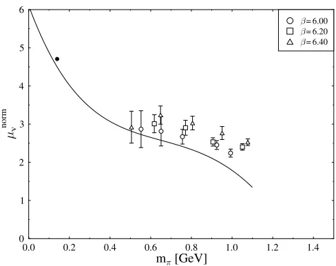
Hemmert and Weise [24] fitted lattice results for the normalized isovector magnetic moment norm

v with the

O.3formula (41) using0v,cVandE r

1 6as fit parame-ters and fixing the other parameparame-ters at their

phenomeno-logical values (see Table V). Their fit yielded a rather strongm_%dependence ofnorm

v for smallm%. The values they obtained for their fit parameters are given in Table VI. A similarly strong m% dependence had already been ob-served in Refs. [25,26] for the magnetic moments of the proton and the neutron. In Fig. 9 we plot our data together with the curve corresponding to the fit of Ref. [24]. The comparison indicates that the data used in Ref. [24] lie somewhat below ours.

B. Combined fits

The results of Ref. [24] show that using the SSE it is possible to connect the experimental value of the magnetic moment with the lattice data. This raises the question whether one could not obtain a similarly good description of the radii by fitting the SSE expression to the simulation results. From the point of view of ChEFT the mass depen-dence of the Dirac and Pauli radius is much simpler to discuss than that of the analogous Sachs quantities. Hence we shall base our analysis onrv₁ andrv₂ instead ofMevand

TABLE VI. Fit values from fits of Eqs. (41) and (49) to lattice data.

Parameter Value from Ref. [24]

0

v 5.1(4)

cV 2:266GeV1

E₁r0:6 GeV 4:9310GeV3

0

s 0:11

E2 0:074 GeV3

0.0 0.2 0.4 0.6 0.8 1.0 1.2 1.4 m [GeV]

0 1 2 3 4 5 6

v

norm

= 6.40 = 6.20 = 6.00

FIG. 9. Our results for the isovector (normalized) magnetic moments compared with the SSE extrapolation curve of Ref. [24]. The solid circle represents the experimental value of v.

TABLE VII. Results of a combined fit (with and without core term) of isovector Pauli radii and anomalous magnetic moments.

Parameter Fitted value Fitted value

Without core term

0v 5.1(8) 4.5(9)

cV 2:35GeV1 2:56GeV1

E₁r0:6 GeV 4:88GeV3 _5:19GeV3

Bc2 0:414GeV3 0:0 GeV3

<2 _{19.2 185.9}

Mvm. Note, however, that the numerical data in the follow-ing discussion are taken from the dipole fits of the Sachs form factors.

Because cut-off effects seem to be small we fitted the results from all three values together taking into account all data points withm%<1 GeV. We keptF%,MN,cAand at their phenomenological values (see Table V), fixed the renormalization scale 6 at 0:6 GeV and chose

B₁₀r0:6GeV 0 for the reason explained in Sec. VIC. Furthermore, we set gA1:2, which is the value in the chiral limit obtained in a recent ChEFT analysis [35] of quenched lattice data. This leaves us with four fit parame-ters:0

v,cV,E r

1 0:6 GeVandBc2. As the Dirac radiusrv1 is independent of these parameters, we performed a simul-taneous fit of rv

22m% and normv m%. The results are collected in the second column of Table VII. Plots of our data together with the fit curves are shown in Figs. 10, 11.

Leaving out the core term inrv

2, i.e.,settingBc20, leads to the parameter values given in the third column of Table VII. The corresponding curves are shown as dashed lines in the figures.

The lattice data for the isovector anomalous magnetic moment are very well described by the chiral extrapolation curve, in particular, if one allows for a (small) core con-tribution via Bc2. Interestingly, the chiral extrapolation function comes rather close to the physical point, although the lightest lattice points are quite far from the physical world and large curvature is required. Moreover, the chiral limit value0vand the values of the other two fit parameters

E₁r andcV in the second column of Table VII compare astonishingly well with the numbers found in Ref. [24] (see Table VI) providing us with some confidence in their determination. The lattice data for the isovector Pauli radius (squared) are also reasonably well described by the chiral extrapolation function of Eq. (47), at least for pion masses below 800 MeV. The effect of the finite core size of the nucleon (parametrized viaBc2) is more visible in this quantity than in v. While the phenomenological value at the physical point is missed by our central curve for rv

2m%, it would lie within the error band, given the relatively large errors of the fit parameters. We note that the

1=m%chiral singularity shows up rather strongly, dominat-ing the curvature out to pion masses around0:3 GeV.

While our generalization of the ChEFT analysis of Ref. [24] describes the ‘‘magnetic’’ quantities _v and rv 2 reasonably well, it is not successful for the isovector Dirac radius. As can be seen in Fig. 10, the chiral extrapolation function drops too fast with m_% and even reaches zero around m%1 GeV. Remember that Dirac radius data 0.0 0.2 0.4 0.6 0.8 1.0 1.2 1.4

m [GeV]

0.0 0.1 0.2 0.3 0.4 0.5 0.6 0.7 0.8 0.9 1.0

(r1 v ) 2 [fm 2 ]

= 6.40 = 6.20 = 6.00

0.0 0.2 0.4 0.6 0.8 1.0 1.2 1.4

m [GeV]

0.0 0.1 0.2 0.3 0.4 0.5 0.6 0.7 0.8 0.9 1.0

(r2 v ) 2 [fm 2 ]

= 6.40 = 6.20 = 6.00

FIG. 10. Isovector radii compared with fit curves. For the fit parameters see Table VII. The dashed line corresponds to the fit without core term. The solid circles represent the experimental values.

0.0 0.2 0.4 0.6 0.8 1.0 1.2 1.4 m [GeV]

0 1 2 3 4 5 6

v

norm

= 6.40 = 6.20 = 6.00

were not included in the fit and the curve shown corre-sponds to the ‘‘no-core term’’ scenario with B₁₀r6

0:6 GeV 0. One could improve the agreement between

the lattice data and the chiral extrapolation curve by allow-ing B₁₀r to provide a positive core contribution, which would shift the curve upwards towards the data. However, this would result in extremely large values for rv

12 at the physical point, as the shape is not modified by

B₁₀r. On the other hand, the simulation data themselves look completely reasonable, indicating that for pion masses around 1 GeV, for which the pion cloud should be considerably reduced, the square of the Dirac radius of the nucleon has shrunk to0:25 fm2_{, less than half of the} value at the physical point. One reason for this failure of Eq. (45) might lie in important higher-order corrections in ChEFT which could soften the strong m% dependence originating from the chiral logarithm.

Nevertheless, one should also not forget that here we are dealing with a quenched simulation. Given thatrv

12at the physical point is nearly completely dominated by the pion cloud (for low values of 6, cf. Equation (46)) it is con-ceivable that the Dirac radius of the nucleon might be sensitive to the effects of (un)quenching. We therefore conclude that especially for rv

1 a lot of work remains to be done, both on the level of ChEFT, where the next-to-leading one-loop contributions need to be evaluated, as well as on the level of the simulations, where a similar analysis as the one presented here has to be performed based on fully dynamical configurations.

Of course, one can think of alternative fit strategies, which differ by the choice of the fixed parameters. For example, one might leave alsoc_Aand free in addition to the four parameters used above. In this (or a similar) way it is possible to force the fit through the data points forrv

12 also, but then the physical point is missed by a considerable amount. So we must conclude that at the present level of accuracy the SSE expression for the Dirac radius is not sufficient to connect the Monte Carlo data in a physically sensible way with the phenomenological value.

C. Beyond the isovector channel

While ChEFT (to the order considered in Ref. [24]) yields the rather intricate expression (41) for the quark-mass dependence of the isovector anomalous magnetic moment, the analogous expression for the isoscalar anoma-lous magnetic moment _spn of the nucleon is much simpler,

_sm_% 0

s8E2MNm2%; (49)

because the Goldstone boson contributions to this quantity only start to appear at the two-loop level [36]. The new countertermE2 parametrizes quark-mass dependent short-distance contributions tos. The error bars of the lattice

data are quite large compared to the small isoscalar anoma-lous magnetic moment. Therefore, any analysis based on (49) and the present lattice results must be considered with great caution, the more so, since the lattice data are also afflicted with the problem of the disconnected contribu-tions. In spite of all these caveats, we now turn to a discussion of the magnetic moments and combinations of them which are not purely isovector quantities.

In Fig. 12 we present the normalized values of s together with a fit using Eq. (49). The values of _s have been computed as _pn from the proton and neutron

0.0 0.2 0.4 0.6 0.8 1.0 1.2 1.4

m [GeV]

-0.6 -0.4 -0.2 0.0 0.2 0.4 0.6

s

norm

= 6.40 = 6.20 = 6.00

FIG. 12. Isoscalar (normalized) anomalous magnetic moments compared with SSE fit. The solid circle represents the experi-mental value ofs. The cross with the attached error bar shows

the value atmphys% .

0.0 0.2 0.4 0.6 0.8 1.0 1.2 1.4

m [GeV]

-3 -2 -1 0 1 2 3

p,n norm

= 6.40 = 6.20 = 6.00

FIG. 13. Anomalous magnetic moments of proton and neutron (normalized) with chiral extrapolation curves. The solid circles represent the experimental values.

dipole fits ofGm, and the errors have been determined by error propagation. We obtain 0s 0:0415 and E2 0:00425 GeV3. These numbers are to be compared with the fit parameters from Ref. [24] given in Table VI. The large statistical errors make definite statements difficult.

Having determined_vm_% as well as _sm_% we can now discuss the chiral extrapolation of proton and neutron data separately. For0

v,cV,E r

1 ,Bc2we choose the values given in the second column of Table VII together with

gA1:2, while for0s andE2 we take the numbers given above and the remaining parameters are fixed at their physical values (see Table V).

In Fig. 13 we compare the resulting extrapolation func-tions with the lattice results for the anomalous magnetic moments. The extrapolation functions are surprisingly well-behaved. Despite the large gap between mphys% and the lowest data point and the substantial curvature involved they extrapolate to the physical point and to the chiral limit in a very sensible way.

Finally, we want to compare our results with the pre-dictions from the constituent quark model. Such compari-sons are usually performed for ratios of observables to avoid normalization problems. Under the assumption that the constituent quark mass mqmumd is equal to

MN=3 also for varying mq, one obtains the well-known

SU6result

p

n

pnorm

n norm

3

2 (50)

and similarly

p

_n norm

p

norm n

1: (51)

In Fig. 14 we show the ratio of the anomalous magnetic moments _p=_n, which is identical to the ratio of the normalized anomalous magnetic moments, as a function of the pion mass. The lattice data and our extrapolation function stay rather close to the staticSU6quark model value of1in the mass range considered here.

VIII. CONCLUSIONS

We have performed a detailed study of the electromag-netic nucleon form factors within quenched lattice QCD employing a fully nonperturbative Oa-improvement of the fermionic action and of the electromagnetic current. Compared with previous studies [4,5] we have accumu-lated much higher statistics, yet our statistical errors appear to be rather large. While these older investigations used one lattice spacing only, we have data at three different lattice spacings. So we could study the discretization errors and found them to be small.

As the quark masses in our simulations are considerably larger than in reality, we had to deal with chiral extrapola-tions. The most effective way to handle this problem proceeds via a suitable parametrization of the Q2 depen-dence of the form factors. Indeed, our data can be de-scribed reasonably well by dipole fits. Then the quark-mass dependence of the fit parameters (dipole quark-masses, in particular) can be studied. Assuming a linear dependence on the pion mass one ends up remarkably close to the physical values, in spite of the fact that the singularities arising from the Goldstone bosons of QCD must show up at some point invalidating such a simple picture. Nevertheless, the difference between the electric and the magnetic dipole mass which we obtain at the physical pion mass is in (semiquantitative) agreement with recent experi-mental results [2,3].

Ideally, the chiral extrapolation should be guided by ChEFT. However, most of the existing chiral expansions do not take into account quenching artefacts and are there-fore, strictly speaking, not applicable to our data. But first simulations with dynamical quarks indicate that at the quark masses considered in this paper quenching effects are small so that quenched chiral perturbation theory is not required. While in this respect the size of our quark masses might be helpful, it leads on the other hand to doubts on the applicability of ChEFT. Indeed, only a reorganisation of the standard chiral perturbation theory series allowed Hemmert and Weise [24] to describe with a single expres-sion the phenomenological value of the isovector anoma-lous magnetic moment of the nucleon as well as 0.0 0.2 0.4 0.6 0.8 1.0 1.2 1.4

m [GeV]

-1.4 -1.2 -1.0 -0.8 -0.6 -0.4 -0.2 0.0

p

/n

= 6.40 = 6.20 = 6.00

FIG. 14. The ratiop=n(identical to the ratio of the