Using Conditioning on Observed Choices to Retrieve Individual-Specific Attribute Processing Strategies

This is a repository copy of

Using Conditioning on Observed Choices to Retrieve

Individual-Specific Attribute Processing Strategies

.

White Rose Research Online URL for this paper:

http://eprints.whiterose.ac.uk/43604/

Article:

Hess, S and Hensher, DA (2010) Using Conditioning on Observed Choices to Retrieve

Individual-Specific Attribute Processing Strategies. Transportation Research Part B:

Methodological, 44 (6). 781 - 790 . ISSN 0191-2615

https://doi.org/10.1016/j.trb.2009.12.001

[email protected] https://eprints.whiterose.ac.uk/ Reuse

Unless indicated otherwise, fulltext items are protected by copyright with all rights reserved. The copyright exception in section 29 of the Copyright, Designs and Patents Act 1988 allows the making of a single copy solely for the purpose of non-commercial research or private study within the limits of fair dealing. The publisher or other rights-holder may allow further reproduction and re-use of this version - refer to the White Rose Research Online record for this item. Where records identify the publisher as the copyright holder, users can verify any specific terms of use on the publisher’s website.

Takedown

If you consider content in White Rose Research Online to be in breach of UK law, please notify us by

1

Using conditioning on observed choices to

retrieve individual-specific attribute

processing strategies

Stephane Hess*

Institute for Transport Studies The University of Leeds [email protected]

David A. Hensher

Institute of Transport and Logistics Studies The University of Sydney

[email protected]

20 November 2008

Abstract

With the growing reliance on Stated Choice (SC) data, researchers are increasingly interested in understanding how respondents process the information presented to them in such surveys.

Specifically, it has been argued that some respondents may simplify the choice tasks by consistently ignoring one or more of the attributes describing the alternatives, and direct questions put to respondents after the completion of SC surveys support this hypothesis. However, in the general context of issues with response quality in SC data, there are certainly grounds for questioning the reliability of stated attribute processing strategies. In this paper, we take a different approach by attempting to infer attribute processing strategies through the analysis of respondent-specific

coefficient distributions obtained through conditioning on observed choices. Our results suggest that a share of respondents do indeed ignore a subset of explanatory variables. However, there is also some evidence that the inferred attribute processing strategies are not necessarily consistent with the stated attribute processing strategies. Additionally, there is some evidence that respondents who claim to have ignored a certain attribute may simply have assigned it lesser importance. The results produced by the inferring approach not only lead to slightly better fit but also more consistent results.

Keywords: stated choice, attribute processing, ignoring attributes, willingness to pay

*

2

Introduction

Information processing strategies play an important role in conditioning the way in which individuals

assess attributes associated with choice alternatives offered in a stated choice experiment (see for example Caussade et al., 2005, Hensher 2006a, Hensher et al. 2007, Hensher, 2008 and Scarpa et al., 2008). Despite a growing number of studies focusing on these issues (see for example Cantillo et al.

2006, Hensher 2006b, Swait 2001, Campbell et al. 2008), in the majority of empirical studies, the entire domain of every attribute is treated as relevant to some degree and included in the utility expressions for every individual. In response to a concern over the assumption of relevancy, a series of papers by Hensher and colleagues in particular have focussed on the role that a range of attribute

processing rules (or heuristics) might play in influencing the empirical identification of the preferences of individuals and populations. These previous research studies have focussed on both the role of self-stated intentions in respect of attendance to attributes (within and between alternatives in a choice set and across choice sets, for example see Puckett and Hensher 2008) as well as the use of economic theory to define a non-linear utility function that can accommodate the degree of attribute attendance up to a probability (see Hensher and Layton 2008, Layton and

Hensher 2008).

Attribute processing has a natural home in psychological theories of choice that assume a dual-phase model of the decision-making process (Houston et al.1989, Kahneman and Tversky, 1979, Thaler, 1999). The first phase relates to the editing of the problem. The second phase relates to the evaluation of the edited problem. The main function to organize and

reformulate the options so as to simplify subse (Kahneman and Tversky, 1979, p. 274). The main function of the evaluation operations is to select the preferred alternative. The accumulating empirical evidence suggests that individuals use a number of strategies derived from heuristics, to represent the way that information embedded within attributes defining alternatives is used to process the context and arrive at a choice outcome. These include cancellation or attribute exclusion, degrees of attention paid to attributes in a package of

attributes, referencing of new or hypothetical attribute packages around a recent or past experience (see e.g. Hess et al., 2008), and attribute aggregation where they are in common units (see Gilovich et al. 2002 for a series of papers that synthesise the evidence under the theme of heuristics and biases). Importantly, as shown herein, the heuristics are likely to be context specific, such that the nature of the information shown in stated choice experiments, for example, conditions the choice of

rules adopted.

While direct questions put to respondents seem to indicate that part of the sample population do indeed consistently ignore certain attributes across choice situations within a given stated choice (SC) experiment, it is not clear whether researchers should rely on this information during model estimation. Firstly, there are arguably issues with endogeneity by conditioning the modelled choice process on stated processing strategies. Hensher (2008) resolved this by treating process and outcome as two related choices. Secondly, the general concern about response quality in SC data clearly extends to such direct questions about decision making, where it perhaps plays an even

bigger role1. As an example, a respondent may indicate that he or she ignored a certain attribute

1

3

whereas in reality they only gave it a lower level of importance than they did for other attributes2. Furthermore, the ignoring may only apply to a subset of choice situations3.

In this paper, we do acknowledge the possibility that some respondents may indeed consistently ignore one or more of the attributes used to describe the alternatives, where the set of ignored

attributes may vary across respondents. However, rather than relying on stated information on ignoring strategies, we attempt to infer such information from the data by making use of post estimation conditioning approaches.

The remainder of this paper is organised as follows. The next section briefly summarises Mixed Logit modelling methodology. This is followed by a discussion of our empirical application. The paper then

closes with the conclusions of our study and makes some suggestions for further research.

Methodology

The random coefficients formulation of the Mixed Multinomial Logit (MMNL) model (cf. Train 2003, Hensher and Greene 2003) is fast becoming one of the most widely used econometric structures for the analysis of travel behaviour. The main advantage of the MMNL model over its more simplistic

closed-form counterparts is that it allows for a relaxation of the assumption of constant marginal utility coefficients across individuals. Here, one of the main topics of interest has been the representation of variations in respondents' valuation of travel time savings (VTTS), i.e., differences in the willingness to pay for reductions in travel time (see for example Hess et al. 2005 and references therein).

Let be the probability of respondent choosing alternative conditional on the vector of taste coefficients , where the specific form for depends on the underlying model type used

in the analysis, such as Multinomial Logit (MNL) or Nested Logit (NL). In a Mixed Multinomial Logit (MMNL) model, we allow for random variations in , where with , the probability for respondent choosing alternative is now given by:

, [1]

i.e. the integral of the conditional MNL choice probability over the distribution of , where the

MMNL choice probability is conditional on .

With giving the alternative chosen by respondent , the log-likelihood function for a cross-sectional model is given by:

, [2]

where gives the total number of respondents.

2

To some extent, such a situation could be better dealt with in the presence of data that also contains respondent-specific ratings for each attribute.

3

4

In a model with multiple choices per respondent, the assumption is generally made that tastes vary across respondents but stay constant across replications for the same respondent. The log-likelihood function then changes to:

, [3]

where gives the alternative chosen by respondent in choice situation (out of ).

In the calibration of MMNL models, we produce estimates of , the vector of parameters of the distribution of . This distribution of works at the level of the sample used in model estimation.

However, after estimation, it is possible to obtain more information on the likely values of for individual respondents by conditioning on the observed choices for specific individuals.

Let define the sequence of observed choices for respondent , and let give the probability of observing this sequence of choices with a specific value for the vector . This would

mean that . Then it can be seen that the probability of observing the

specific value of given the choices of respondent is given by:

, [4]

from which it is straightforward to produce moments of the conditional distribution of for each

respondent.

Empirical application

Data

The data used in this application were collected in Sydney in 2004. In a face-to-face computer aided personal interview (CAPI), respondents were faced with sixteen separate choice situations. In each

The three alternatives were described by five attributes, namely free flow time, slowed down time, trip travel time variability, vehicle running cost and toll cost. A D-efficient design was used in the generation of the SC questionnaires (see for example Rose et al. 2008). For a more detailed

description of the survey in the context of a recent application, see Hess et al. (2008).

After completing the SC part of the survey, respondents were asked to indicate whether they ignored any of the attributes over the course of the sixteen choice situations they were faced with. The specific wordi Please indicate which of the following attributes you ignored when

Model specification

A linear formulation of the utility function was used, and in addition to the five marginal utility coefficients, alternative specific constants were included for the first two alternatives. On the basis of this, the base utility function for alternative i is given by:

5

where and define the free flow and slowed down time of alternative respectively, with and being running cost and toll charges, while is the travel time variability for alternative . The alternative specific constant is set to zero for the third alternative.

Estimation results

For the present analysis, a sample of 3,280 observations is used, collected from 205 non-commuters. Various versions of the MMNL models were estimated, making use of Normal, Lognormal, Triangular and Uniform distributions. Additionally, all models were estimated with independently distributed as well as correlated marginal utility coefficients. The findings in terms of information processing strategies were broadly comparable (i.e. which respondents were allocated to the ignoring and

non-ignoring classes), and for illustration purposes, we limit ourselves here to the results for the model using independent Normal distributions for the random coefficients4.

Base models

We first look at the estimation of two base models, with results summarised in Table 1. These models, one MNL and one MMNL, take no account of differences across respondents in their information processing strategies, although a case could be made that the MMNL model gives

partial recognition to the ignoring of attributes by allowing for differences in marginal utility coefficients across respondents, with the Normal distribution giving a positive probability to a coefficient value arbitrarily close to zero.

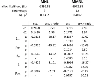
Table 1: Estimation results for base models

MNL

MMNL

Final log likelihood (LL) -2395.88 -1972.88

parameters 7 12

2

0.3332 0.4492

est. asy. t-ratio est. asy. t-ratio

0.2858 3.59 0.3918 2.99

0.1480 2.56 0.1472 1.94

FFT

-0.0813 -20.17 -0.1357 -12.07

- - 0.1330 8.85

SDT

-0.0926 -19.92 -0.1416 -13.08

- - 0.1014 9.50

RC

-0.3645 -14.92 -0.5862 -11.25

- - 0.4580 8.10

T

-0.4429 -31.01 -0.8916 -16.37

- - 0.5082 12.00

VAR

-0.0087 -2.59 -0.0191 -2.13

- - 0.0757 10.22

In both models, all marginal utility coefficients obtain high levels of statistical significance and are of the correct sign. The results for the alternative specific constants show a high level of inertia for the

4

6

base alternative, along with some evidence of a reading left to right effect. We obtain highly significant improvements in model fit when moving from MNL to MMNL, with high levels of random taste heterogeneity for all five marginal utility coefficients.

Models conditioning on stated IPS

In our next set of models, we take the stated ignoring strategies into account. The strategies reported by respondents are summarised in Table 2, showing variable rates of ignoring, with high rates for running costs and travel time variability.

Table 2: Stated ignoring strategies

Attribute ignored Respondents Rate

Free flow travel time 26 12.68%

Slowed down travel time 32 15.61%

Running costs 59 28.78%

Toll 18 8.78%

Travel time variability 61 29.76%

Given the earlier discussion about the validity of stated attribute processing strategies, our models do not simply condition on stated ignoring, but test the accuracy of the data in this context. Specifically, instead of setting coefficients in the stated ignoring group to zero, we estimate separate coefficients in this group, with the alternative specific constants remaining generic. If respondents

truly ignored the concerned attributes across all sixteen choice situations, the associated coefficients in the ignoring group should be equal to zero. The results are summarised in Table 3.

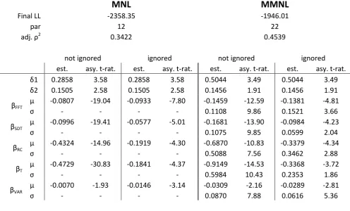
Table 3: Models based on stated information processing strategies

MNL

MMNL

Final LL -2358.35 -1946.01

par 12 22

2

0.3422 0.4539

not ignored ignored not ignored ignored

est. asy. t-rat. est. asy. t-rat. est. asy. t-rat. est. asy. t-rat.

0.2858 3.58 0.2858 3.58 0.5044 3.49 0.5044 3.49

0.1505 2.58 0.1505 2.58 0.1456 1.91 0.1456 1.91

FFT

-0.0807 -19.04 -0.0933 -7.80 -0.1459 -12.59 -0.1381 -4.81

- - - - 0.1108 9.86 0.1521 3.66

SDT

-0.0996 -19.41 -0.0577 -5.01 -0.1681 -13.90 -0.0984 -4.23

- - - - 0.1075 9.85 0.0599 2.04

RC

-0.4324 -14.96 -0.1919 -4.30 -0.6870 -10.83 -0.3379 -4.34

- - - - 0.5088 7.56 0.3462 2.88

T

-0.4729 -30.83 -0.1841 -4.37 -0.9149 -14.53 -0.3368 -3.72

- - - - 0.5984 10.43 0.2353 1.86

VAR

-0.0070 -1.93 -0.0146 -3.14 -0.0309 -2.16 -0.0289 -2.81

7

Our analysis shows that the models conditioning on stated information processing strategies obtain

statistically significant improvements over the base models, with test values of 75.06 and 53.74 for MNL and MMNL respectively, and critical 99% test values of 15.08 and 23.21 respectively. These improvements in model fit suggest that there are indeed significant differences in marginal utility coefficients between respondents who state that they did or did not ignore a certain attribute in their decision making process. However, a closer inspection of our results shows that, in the MNL model, the coefficients in the ignoring part of the sample are still all significantly different from zero, with the same applying for the mean values of the coefficients in the MMNL model, where there are also still high levels of variations in sensitivities across respondents in the ignoring part of the sample. Looking specifically at the degree of heterogeneity (i.e. standard deviation relative to mean), we can observe that when moving from the model in Table 1 to the model in Table 3, the degree of heterogeneity in the non-ignoring part is lower than in Table 1 for all coefficients except the toll coefficient. In the ignoring part of the sample, the degree of heterogeneity is higher than in the non-ignoring part for the free flow travel time coefficient, the running cost coefficient and the toll coefficient. These results hence suggest the presence of quite different patterns of heterogeneity in the two groups.

As a next step, we look at the differences in sensitivities across the two groups, where we focus on the mean values of the coefficients. These results are summarised in Table 4. We observe that, in

MNL FFT VAR in the ignoring part of the sample are in fact

F SDT RC

T, the sensitivities in the ignoring part of the sample are lower than in the remaining part of the

sample, but remain significantly larger than zero. In the MMNL model, the situation is very similar. The mean values for all five coefficients are now lower in the ignoring part, with the differences between the two groups being significant for SDT, RC and T. As pointed out above, the degree of

heterogeneity in the ignoring part of the sample is higher for FFT, RC and T.

Table 4: Differences between groups conditioned on stated information processing strategies (mean coefficient values only)

MNL

MMNL

difference

(ign. vs not ign.) asy. t-rat.

difference

(ign. vs not ign.) asy. t-rat.

FFT -0.0126 -1.01 0.0078 0.25

SDT 0.0419 3.37 0.0697 2.70

RC 0.2405 4.59 0.3491 3.53

T 0.2888 6.51 0.5781 5.32

VAR -0.0076 -1.68 0.0020 0.13

On balance, this experiment has shown that there do indeed seem to be differences in marginal sensitivities between respondents in the two groups, with generally lower sensitivities for respondents who claim to have ignored a certain attribute. However, the estimates in the ignoring

part of the sample remain statistically significant, suggesting that it is not appropriate to rely on stated ignoring information by setting the concerned coefficients to a value of zero. The lower

8

attributes defining the package, or perhaps that they simply assigned a lower level of importance to these attributes, a possibility discussed in the introduction to this paper.

Inferring IPS through conditioning on observed choices

In the next phase of our analysis, we aim to infer the ignoring strategies through a posterior analysis of the MMNL estimates by conditioning on observed choices. To this extent, the mean and standard deviation for the conditional distribution were calculated for each of the five marginal utility coefficients and each of the 205 respondents, on the basis of the MMNL results from Table 1.

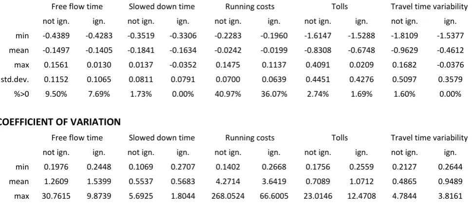
As a first step, we use these conditional parameters to investigate differences between the two groups obtained though segmenting according to the stated ignoring strategies. The findings of this process are summarised in Table 5 which looks at the mean of the conditional distribution along with the coefficient of variation.

In terms of conditional means, the positive values obtained for some respondents can be explained by the use of the Normal distribution (cf. Hess et al., 2005). For the differences between the two groups, we observe a narrower range and a lower mean in the ignoring part of the sample, consistent with the MMNL estimation results from Table 3. Looking at the coefficient of variation,

we observe (with the exception of RC), a higher value for the ignoring part of the sample, along with

a narrower range.

On the basis of the results from Table 3 and Table 5, we cannot completely reject the idea that some respondents in our sample do indeed consistently ignore certain attributes in their decision making. However, our results from Table 3 also show that relying purely on the deterministic representation

of stated information processing strategies can lead to inconsistent results5.

Table 5: Analysis of conditional parameters in data segmented by stated information processing strategies

CONDITIONAL MEANS

Free flow time Slowed down time Running costs Tolls Travel time variability not ign. ign. not ign. ign. not ign. ign. not ign. ign. not ign. ign. min -0.4389 -0.4283 -0.3519 -0.3306 -0.2283 -0.1960 -1.6147 -1.5288 -1.8109 -1.5377 mean -0.1497 -0.1405 -0.1841 -0.1634 -0.0242 -0.0199 -0.8308 -0.6748 -0.9629 -0.4612 max 0.1561 0.0130 0.0137 -0.0352 0.1475 0.1137 0.4091 0.0209 0.1682 -0.0376 std.dev. 0.1152 0.1065 0.0811 0.0791 0.0700 0.0639 0.4451 0.4276 0.5097 0.3579 %>0 9.50% 7.69% 1.73% 0.00% 40.97% 36.07% 2.74% 1.69% 1.60% 0.00%

COEFFICIENT OF VARIATION

Free flow time Slowed down time Running costs Tolls Travel time variability not ign. ign. not ign. ign. not ign. ign. not ign. ign. not ign. ign. min 0.1976 0.2448 0.1069 0.2707 0.1402 0.2668 0.1756 0.2559 0.2127 0.2644 mean 1.2609 1.5399 0.5537 0.5683 4.2714 3.6419 0.7089 1.0712 0.4865 0.9489 max 30.7615 9.8739 5.6925 1.8044 268.0524 66.6005 23.0146 12.4708 4.7844 3.8161

We now turn to the use of the parameters of the conditional distributions in our attempt to retrieve ignoring strategies from the data. Simply allocating respondents on the basis of the means of the

5

9

conditional distributions seems inappropriate. Indeed, a respondent may have very low sensitivity to an attribute without actually ignoring it. This would lead to a low mean for the conditional distribution for that coefficient and that respondent, and working solely on the basis of this

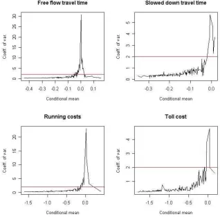
conditional mean would thus incorrectly allocate this respondent to the ignoring part of the sample population. What we want in effect is a measure that tells us when the conditional mean is indistinguishable from zero. To incorporate the uncertainty in the conditional distributions, we put forward the idea of working with the coefficient of variation, i.e. the ratio between the standard deviation and the mean of the conditional distribution. In our application, a high coefficient of variation is only obtained for respondents who have a very low conditional mean (virtually zero), a claim that is supported by the evidence in Figure 1 which shows a plot of the coefficient of variation

values for the four main coefficients6 and 205 respondents, sorted by the values for the conditional mean.

Figure 1: Coefficient of variation for conditional distributions

While working with the coefficient of variation incorporates uncertainty into our approach, the task still remains to decide how to allocate respondents to different groups on the basis of the coefficient of variation. In this analysis, we work with a trial value of 2, so that a respondent with a coefficient of variation above this value will be allocated to the ignoring part of the sample. The choice of a value of 2 is a rather arbitrary but conservative threshold, and more work is required to evaluate the impact of the threshold choice on results. One possibility in this context would be to use an iterative

search to determine the optimal value for this threshold.

6

10

Table 6 summarises the allocation into the ignoring group obtained when using a threshold of 2 for the coefficient of variation for the conditional distributions. The results show a higher rate for free flow time than in the stated information, while the rates are much lower for slowed down time,

running costs and tolls. Finally, the rate of ignoring for travel time variability is virtually identical.

Table 6: Ignoring strategies retrieved by conditioning on observed choices

Attribute ignored Respondents Rate

Free flow travel time 32 15.61%

Slowed down travel time 5 2.44%

Running costs 11 5.37%

Toll 4 1.95%

Travel time variability 60 29.27%

Aside from the actual rates of ignoring with the two approaches, the allocation of specific individuals

to the two groups is of interest. Here, some worrying differences arise between the stated and

inferred information processing strategies, as highlighted in Table 7.

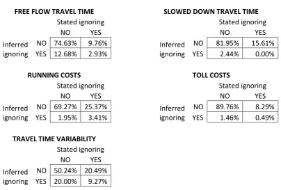
Table 7: Comparison of stated and inferred ignoring strategies

FREE FLOW TRAVEL TIME SLOWED DOWN TRAVEL TIME

Stated ignoring Stated ignoring

NO YES NO YES

Inferred ignoring

NO 74.63% 9.76% _Inferred

ignoring

NO 81.95% 15.61%

YES 12.68% 2.93% YES 2.44% 0.00%

RUNNING COSTS TOLL COSTS

Stated ignoring Stated ignoring

NO YES NO YES

Inferred ignoring

NO 69.27% 25.37% _Inferred

ignoring

NO 89.76% 8.29%

YES 1.95% 3.41% YES 1.46% 0.49%

TRAVEL TIME VARIABILITY Stated ignoring

NO YES

Inferred ignoring

NO 50.24% 20.49%

YES 20.00% 9.27%

Starting with free flow travel time, we have already mentioned the slightly higher rate of ignoring when working on the basis of the inferred processing strategies (15.61% vs 12.68%)7. However, other differences arise. Indeed, only 77.56% of respondents get allocated to the same groups with the two approaches, while 12.68% of the sample fall into the inferred ignoring group despite not indicating ignoring behaviour when asked after the SC survey. The remaining 9.76% of the sample

7

11

indicated that they had in fact ignored free flow time, but are allocated into the not ignored group when working with the inferred strategies.

Turning to slowed down time, we not only observe a much lower rate of ignoring when working with the retrieved strategies, but also note that any respondent allocated to the ignoring group with either approach in fact falls into the not ignored group with the other approach.

For running costs, the rates are again much lower when working with retrieved strategies, and the majority of respondents (25.37% out of 28.78%) who stated that they ignored running costs actually fall into the not ignored group when working with the retrieved strategies. The picture for tolls is very similar, with almost no ignoring in the retrieved strategies, compared to 8.78% in stated

strategies.

Looking finally at travel time variability, we observe virtually identical rates of ignoring with the two approaches. However, the allocation to the two groups is the same with the two approaches for only 59.51% of respondents, where, when looking at the ignoring parts only, the rates of false allocation are of the order of 68-69% depending on which approach is taken to be correct.

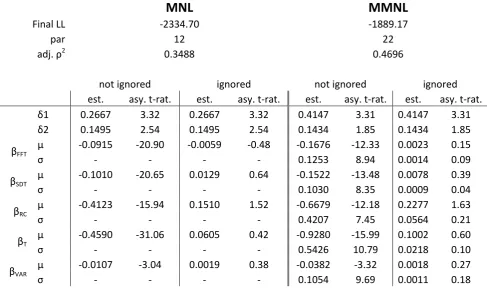
As a test of the validity of our inferred ignoring strategies, we estimated a new set of models that

are the equivalent of the models from Table 3 but with the conditioning being on the inferred as opposed to stated ignoring strategies. In other words, like in Table 3, separate coefficients were again estimated for the ignoring and not ignoring groups, but this time the group allocation was based on the coefficients of variation approach rather than on the stated strategies. The results for these models are summarised in Table 8.

Table 8: Models based on inferred information processing strategies

MNL

MMNL

Final LL -2334.70 -1889.17

par 12 22

2

0.3488 0.4696

not ignored ignored not ignored ignored

est. asy. t-rat. est. asy. t-rat. est. asy. t-rat. est. asy. t-rat.

0.2667 3.32 0.2667 3.32 0.4147 3.31 0.4147 3.31

0.1495 2.54 0.1495 2.54 0.1434 1.85 0.1434 1.85

FFT

-0.0915 -20.90 -0.0059 -0.48 -0.1676 -12.33 0.0023 0.15

- - - - 0.1253 8.94 0.0014 0.09

SDT

-0.1010 -20.65 0.0129 0.64 -0.1522 -13.48 0.0078 0.39

- - - - 0.1030 8.35 0.0009 0.04

RC

-0.4123 -15.94 0.1510 1.52 -0.6679 -12.18 0.2277 1.63

- - - - 0.4207 7.45 0.0564 0.21

T

-0.4590 -31.06 0.0605 0.42 -0.9280 -15.99 0.1002 0.60

- - - - 0.5426 10.79 0.0218 0.10

VAR

-0.0107 -3.04 0.0019 0.38 -0.0382 -3.32 0.0018 0.27

12

In a direct comparison across models (based on the adjusted 2 measures), we note that the models conditioning on inferred ignoring strategies not only outperform the base models from Table 1, but likewise outperform the models conditioning on stated ignoring strategies in Table 3. More importantly however, our results show that in both the MNL and MMNL model, none of the marginal utility coefficients are statistically significant8, where the positive sign of the estimates is consequently of little importance. Finally, the results show a lower degree of heterogeneity

throughout when compared to the models in Table 1, with the exception of T,where the difference

is only very small. This would suggest that some of the heterogeneity retrieved in the MMNL model in group 1 is in fact an artefact of the presence of some respondents who ignore the relevant attribute (i.e. have a zero coefficient).

Overall, this test could suggest that the inferred ignoring strategies are indeed more accurate than the stated ignoring strategies, with the results supporting the hypothesis that respondents in our

inferred ignoring group did indeed ignore the values of the concerned attributes. However, the fact that when working with the stated ignoring strategies, the coefficients in the ignoring part of the sample are lower than in the remainder of the sample does similarly suggest some differences in behaviour in the two groups when conditioning on stated behaviour. Potentially, the stated ignoring groups comprise some individuals who ignored the attributes only in some of the choice situations, supporting the view that such supplementary questions should be asked after each choice set (as

was the case in Puckett and Hensher 2008).

Summary and conclusions

This paper has discussed issues arising in the presence of respondents who consistently ignore one or more of the attributes describing alternatives in SC surveys. Specifically, we have contrasted two approaches to identify such respondents, one of them being based on direct questions put to respondents, while the other one aims to infer such ignoring behaviour through an a posteriori analysis that conditions on observed choices. Both approaches produce evidence that some of the respondents do indeed ignore certain of the attributes in their decision making. However, there are some inconsistencies between the two approaches in terms of the rates of ignoring as well as the allocation of specific respondents to the ignoring and not ignoring groups. Additionally, it should be said that the approach conditioning on inferred strategies does produce slightly better model fit and

also produces more consistent results in the ignoring part of the population (i.e. zero valuations). A possible explanation for the results in this paper is that some of the respondents who indicate that they ignored a certain attribute only did so for a subset of their choice situations, despite the fact that the wording of the question put to respondents was quite clear. Additionally, there is a possibility that they did not in fact ignore an attribute, but simply attached lower importance to it, a

hypothesis supported by the lower marginal sensitivities in the ignoring segment.

In relation to the point about the ignoring only applying to a subset of the choice sets, a separate analysis was undertaken to test for variations across the sixteen choices for each respondent. In the

8

RC obtains the highest levels of significance, with rates of 87.15% and 89.69% in the MNL and MMNL model

13

first instance, we tested for differences by estimating choice set specific scale parameters, where the results showed no significant differences in the relative weight of the error term across the sixteen choices. To test for differences in the relative (as opposed to absolute) marginal utilities, we also

estimated models separately for different subsets of the choice sets (e.g. separate models for first eight and last eight choices) and again the results did not provide conclusive evidence to suggest that the observations from different choice sets should be treated separately.

More work remains to be done, including refining the conditioning approach and defining a less arbitrary way of allocating respondents to the different groups. The approach can also be extended to test for other processing strategies such as respondents evaluating multiple attributes jointly rather than separately. Considering stated non-attendance to attributes after each choice set, in

contrast to after all choice sets, takes into account the level of the attribute as well and this may be an important feature, given evidence that WTP is most sensitive to the levels and ranges of attribute levels in a stated choice experiment. Finally, more work needs to be done in understanding the stated information processes, and there is potential benefit in combining the two approaches9. We do believe, given the evidence, that attribute processing strategies play an important role in choice

making, and that the challenge ahead is to find ways of better representing the way that specific attributes in an attribute package are treated by individuals when making specific choices, be they in real or hypothetical market situations.

In closing, it is worth briefly contrasting our proposed approach to a latent class approach in which we allow for separate classes depending on ignoring strategies, with the coefficients values fixed to zero in one class. The class allocation probabilities for the zero value class then give an indication of the incidence of ignoring in the sample population. This approach has for example been advocated by Hess & Rose (2007) Hensher & Greene (2008). A possible problem with this approach however is that the zero value class may not only capture respondents who ignore an attribute but also those whose marginal utilities are closer to zero than they are to the mode of the true distribution (represented by the non-zero value class). It could be argued that the approach used in the present paper is less susceptible to such confounding as we allocate respondents based on their conditional

distributions rather than based on whether their sensitivities are closer to zero than to the mode of the distribution.

References

C D W G H “ ‘ I D P

A D C E Environmental andResource Economics, in press. Cantillo, V., Heydecker, B. and Ortuzar, J. de Dios (2006): A Discrete Choice Model Incorporating

Thresholds for Perception in Attribute Values , Transportation Research B, 40 (9), 807-825.

9

14

Caussade, S., Ortúzar, Juan de Dios Ortúzar, J., Rizzi L. and Hensher, D.A. (2005) Assessing the Influence of Design Dimensions on Stated Choice Experiment Estimates, Transportation Research B, 39 (7), 621-640.

Gilovich, T., Griffin, D. and Kahneman, D. (Eds.) (2002): Heuristics and Biases The Psychology of Intuitive Judgment, Cambridge University Press, Cambridge.

H D A A Valuing Environmental

Amenities using Stated Choice Studies: A Common Sense Approach to Theory and Pra Barbara Kanninen, ed., Springer, Dordrecht, The Netherlands, 135-158

Hensher, D.A. (2006b) How do Respondents Process Stated Choice Experiments? Attribute consideration under varying information load, Journal of Applied Econometrics, 21, 861-878 Hensher, D.A. (2008) Joint estimation of process and outcome in choice experiments and

implications for willingness to pay, Journal of Transport Economics and Policy, 42 (2), May, 297-322.

Hensher, D.A. and Greene, W. (2003), The Mixed Logit Model: The State of Practice, Transportation, 30 (2), pp. 133-176.

H D A G W H N -Attendance and Dual Processing of Common-Metric

Attributes in Choice Analysis: A Latent Class Specification , Department of Economics, New York University, August

H D A L D A T N

-Institute of Transport and Logistics Studies, University of Sydney.

Hensher, D.A., Rose, J. and Bertoia, T. (2007) The implications on willingness to pay of a stochastic treatment of attribute processing in stated choice studies, Transportation Research E, 43 (1), 73-89.

Hess, S., M. Bierlaire and J. W. Polak (2005) Estimation of value of travel-time savings using mixed logit models, Transportation Research A, 39 (2-3) 221 236.

Hess, S., Rose, J. M. and Hensher, D.A. (2008) Asymmetrical preference formation in Willingness to Pay Estimates in Discrete Choice Models, Transportation Research E, 44(5), pp. 847-863.

Hess, S. & Rose, J.M. (2007), A latent class approach to modelling heterogeneous information processing strategies in SP studies, paper presented at the Oslo Workshop on Valuation Methods in Transport Planning, Oslo.

H D A “ “ J B “ M T I fluence Of Unique Features And D O C O P Journal of Experimental Social Psychology, 25, 121 141.

K D T A P T A A D U ‘

Econometrica, 47 (2), 263-91.

L D H D A A C -Metric Attributes in Preference

‘ C E I W P

Transportation Research D Special Issue, May 15, 2008.

Puckett, S.M. and Hensher, D.A. (2008) The role of attribute processing strategies in estimating the preferences of road freight stakeholders under variable road user charges, Transportation Research E, 44, 379-395.

Rose, J.M., Bliemer, M.C., Hensher and C A T D

Transportation Research B 42 (4), 395-406

Scarpa, R., Gilbride, T., Campbell, D. and Hensher, D.A. (2008): Modeling attribute non-attendence in choice experiments: does it matter? Submited to American Journal of Agricultural Economics.

“ J A N -Compensatory Choice Model Incorporating Attribute Cut-O

Transportation Research B, 35(10), 903-928.

15

Train, K. (2003) Discrete Choice Methods with Simulation, Cambridge University Press, Cambridge, MA.