A direct forcing immersed boundary method employed with compact integrated RBF approximations for heat transfer and fluid flow problems

A direct forcing immersed boundary method employed with compact integrated RBF approxima-tions for heat transfer and fluid flow problems

N. Thai-Quang, N. Mai-Duy, C.-D. Tran and T. Tran-Cong

Computational Engineering and Science Research Centre, Faculty of Health, Engineering and Sciences, The University of Southern Queensland, Toowoomba, Queensland 4350, Australia.

Abstract: In this paper, we present a numerical scheme, based on the direct forcing immersed bound-ary (DFIB) approach and compact integrated radial basis function (CIRBF) approximations, for solving the Navier-Stokes equations in two dimensions. The problem domain of complicated shape is embedded in a Cartesian grid containing Eulerian nodes. Non-slip conditions on the inner boundaries, represented by Lagrangian nodes, are imposed by means of the DFIB method, in which a smoothed version of the discrete delta functions is utilised to transfer the physical quantities between two types of nodes. The velocities and pressure variables are approximated locally on Eulerian nodes using 3-node CIRBF sten-cils, where first- and second-order derivative values of the field variables are also included in the RBF approximations. The present DFIB-CIRBF scheme is verified through the solution of several test prob-lems including Taylor-Green vortices, rotational flow, lid-driven cavity flow with multiple solid bodies, flow between rotating circular and fixed square cylinders, and natural convection in an eccentric annu-lus between two circular cylinders. Numerical results obtained using relatively coarse grids are in good agreement with available data in the literature.

Keywords: compact integrated RBF, immersed boundary, direct forcing, viscous flow, heat transfer.

1 Introduction

Flows past solid bodies of arbitrary shapes are widely encountered in engineering applications. Body-fitted grid methods, where the governing equations are discretised on a curvilinear grid conforming to the boundary, have been applied to solve such problems. Their main advantage is that the boundary conditions can be imposed in a simple and accurate way. However, generating a high quality mesh/grid is difficult and time-consuming. As a result, a lot of research effort has been spent on the development of non-body-conforming methods. Among them, the immersed boundary methods (IBMs) have received much attention in recent years. In IBMs, one joins the fluid and solid regions together to make a single domain that is discretised using a Cartesian grid. This approach greatly simplifies the process of mesh generation and also retains the relative simplicity of the governing equations. The basis of IBMs lies in the way to introduce forces into the governing equations to impose prescribed values on the immersed boundary.

forcing approach to iteratively determine the magnitude of the force required to obtain a desired veloc-ity on the immersed boundary. Saiki and Biringen (1996) implemented this approach with the virtual boundary method (VBM) to compute the flow past a stationary, rotating and oscillating circular cylin-der. However, the feedback forcing approach induces some oscillations and places some restriction on the computational time step. To overcome these drawbacks, Fadlun, Verzicco, Orlandi, and Mohd-Yusof (2000) proposed an approach, namely the direct forcing (DF) technique, to evaluate the interactive forces between the immersed boundary (IB) and the fluid, which is equivalent to applying a forcing term to the Navier-Stokes equations. In comparison with the feedback forcing approach, the DF approach can work with larger computational time steps. Kim, Kim, and Choi (2001) proposed a combined IB finite-volume method, where a mass source/sink and a momentum forcing are introduced, for simulating flows over complex geometries. To transfer the physical quantities smoothly between Eulerian and Lagrangian nodes and avoid strong restrictions on the time step, Uhlmann (2005) presented a method to incorporate the regularised delta functions into a direct formulation of the fluid-solid interactive force. Wang, Fan, and Luo (2008) developed an explicit multi-direct forcing approach and obtained a better satisfaction of the non-slip boundary condition than the original DF approach. Recently, Ji, Munjiza, and Williams (2012) proposed an iterative IBM in which the body force updating is incorporated into the pressure iterations for the two- (2D) and three-dimensional (3D) numerical simulations of laminar and turbulent flows. The reader is referred to, e.g., Mittal and Iaccarino (2005) for a comprehensive review of IBMs. High-order approximation schemes for the Navier-Stokes equations have the ability to provide efficient solutions to steady/unsteady fluid flow problems. A high level of accuracy can be achieved using a relatively coarse discretisation. Many types of high-order schemes for the Navier-Stokes equations have been reported in the literature. Botella and Peyret (1998) developed a Chebyshev collocation method and provided the benchmark results for the lid-driven cavity flow problem. Ding, Shu, Yeo, and Xu (2006) presented a local multiquadric differential quadrature method for the solution of 3D incompressible flow problems in the velocity-pressure formulation, while Mai-Duy and Tran-Cong (2001b), Mai-Duy, Le-Cao, and Tran-Cong (2008), Mai-Duy and Tran-Cong (2008), Le-Le-Cao, Mai-Duy, and Tran-Cong (2009) proposed an integrated-RBF (IRBF) method to solve heat transfer and fluid flow problems in the stream function-vorticity formulation. Recently, Tian, Liang, and Yu (2011) proposed a fourth-order compact difference scheme constructed on 2D nine-point stencils, and Fadel and Agouzoul (2011) used the stan-dard Padé scheme to construct high-order approximations for the velocity-pressure-pressure gradient formulation. It is noted that the velocity (u) and pressure (p) formulation has several advantages over the stream function-vorticity formulation and the stream function formulation. The u-p formulation can provide the velocity and pressure fields directly from solving the discretised equations and also work for 2D and 3D problems in a similar manner.

fourth-order PDEs [Mai-Duy and Tanner (2007)] and compact local forms for second-fourth-order elliptic problems [Mai-Duy and Tran-Cong (2011); Mai-Duy and Tran-Cong (2013)]. For the latter, the information about the governing equation or derivatives of the field variable is also included in local approximations to enhance the solution accuracy.

In this paper, we present a numerical scheme, namely DFIB-CIRBF, for solving unsteady/steady fluid flow problems in 2D. The present scheme combines the direct forcing immersed boundary (DFIB) method and the high-order compact integrated radial basis function (CIRBF) approximations for the spatial discretisation and utilises the second-order Adams-Bashforth/Crank-Nicolson algorithms for the temporal discretisation. An interactive force, representing the effect of the solid bodies on the fluid re-gion, is added directly to the governing equations (i.e. direct forcing) on the fluid-solid regions to satisfy their boundary conditions. This interactive force is evaluated explicitly from the pressure gradient, the convection and diffusion terms in the previous time level. Because the Eulerian grid nodes do not gen-erally coincide with the nodes on the interfaces represented by Lagrangian nodes, a smoothed version of the discrete delta functions is employed to transfer the quantities between two types of nodes. The CIRBF approximations are constructed over 3-point stencils, where nodal first- and second-order deriva-tive values of the field variables are included in the RBF approximations [Thai-Quang, Mai-Duy, Tran, and Tran-Cong (2012)]. A series of test problems, including Taylor-Green vortices, rotational flow, flow between rotating circular and fixed square cylinders, and natural convection in an eccentric annulus be-tween two circular cylinders, is considered to verify the present scheme. The remainder of the paper is organised as follows. Section 2 outlines the equations which govern the fluid flow phenomena. The numerical formulation including the derivation of interactive forces, and the temporal and spatial dis-cretisations is described in detail in Section 3. In Section 4, in order to evaluate the efficiency of the present method, several numerical results are presented and compared with the analytic solutions and some approximate results available in the literature, where appropriate. Section 5 concludes the paper.

2 Governing equations

The IB approach takes the Navier-Stokes equation for thermal flows in the dimensionless form as follows

∇.u=0 in Ω, (1)

∂u

∂t + (u.∇)u=−∇p+

r

Pr Ra∇

2_{u+fb+fI in Ω, (2)}

∂T

∂t + (u.∇)T = 1 √

PrRa∇ 2_T+f

I,T in Ω, (3)

subject to the initial and boundary conditions:

u(x,y,0) =u0(x,y) in Ω, (4)

u(x,y,t) =u_Γ(x,y,t) on Γ, (6)

T(x,y,t) =TΓ(x,y,t) on Γ, (7)

where Ωis the entire domain of analysis that is of simpler shape than the fluid domain; u= (u,v)T, p and T the velocity vector, the static pressure and the temperature, respectively; fb = fb,x,fb,yT, fI = (fI,x,fI,y)T and fI,T the body-force vector, the momentum interactive force vector and the thermal interactive force, respectively; u0, uΓ, T0and TΓprescribed functions; Pr and Ra the Prandtl and Rayleigh numbers defined as Pr=ν/αand Ra=βg∆T L3/αν, respectively, in whichνis the kinematic viscosity, αis thermal diffusivity,βthe thermal expansion coefficient, g the gravity and L and∆T the characteristic length and temperature difference, respectively. In the dimensionless form, the characteristic velocity is taken as U0=pgLβ∆T for the purpose of balancing the buoyancy and inertial forces.

In (1), (2) and (3), the field variables are made dimensionless according to the following definitions

x=x′

L,y= y′ L,u=

u′ U0

,v= v′

U0

, p= p′

ρU₀2,T =

T′₋Tc Th−Tc

, (8)

where x′, y′, u′, v′, p′, T′ are the corresponding dimensional variables; and Th and Tc the hot and cold temperatures, respectively.

The interactive forces fI and fI,T represent the influence of the immersed solid bodies on the fluid by the viscous and thermal effects, while the body force fb is a function of the temperature, for instance, fb= (0,T)T for the thermal problem considered in Section 4. For isothermal flows, the term fbin (2) is set to null, equation (3) is deactivated and the term

q

Pr

Ra in (2) is replaced by 1

Re where Re=U0L/νis the Reynolds number.

3 Numerical formulation

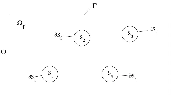
Consider a domainΩcomprised of the fluid regionΩf and solid regionΩs. The latter is composed of Nesb embedded solid bodies Sk

Ωs=SNesb

k=1Sk

as shown in Figure 1. LetΓand∂Sk be the boundaries ofΩ and kth solid body Sk, respectively. While the entire domainΩis discretised using a fixed uniform Carte-sian grid gh containing Eulerian grid nodes xi,j = (xi,j,yi,j)T (i∈ {1,2, . . . ,nx}and j∈ {1,2, . . . ,ny}), each∂Sk is described by a set of NLkLagrangian nodes

Xk_l =X_lk,Y_lk

T

∈∂Sk 1≤l≤NLk,1≤k≤Nesb. (9)

3.1 Direct forcing method

desired velocity and temperature values, respectively, at selected Eulerian nodes near the IB. An inter-polation process is necessary to transfer data between the selected Eulerian nodes and the Lagrangian nodes on the IB. Below are the details for computing the momentum interactive force fIin (2). One can calculate the thermal interactive force fI,T in (3) in a similar manner.

3.1.1 Derivation of the momentum interactive force

A temporal discretisation of the momentum equation (2) is given by Uhlmann (2005)

un₋un−1 ∆t =rhs

n−1/2_+fn−1/2

I , (10)

where the superscript n denotes the current time level; the convection, pressure, diffusion and body-force terms at a time tn−1/2are lumped together in rhsn−1/2.

The interactive force term yielding the desired velocity u(d) can thus be defined as [Fadlun, Verzicco, Orlandi, and Mohd-Yusof (2000)]

fn_I−1/2=u

(d),n_−un−1 ∆t −rhs

n−1/2_{, (11)}

at some selected nodes (and zero elsewhere). The corresponding interactive force at the Lagrangian nodes will be

Fn_I−1/2=U

(d),n_−Un−1

∆t −RHS

n−1/2_{. (12)}

Hereafter, we use upper-case letters for quantities evaluated at the Lagrangian nodes Xk_l.

The desired velocity at a node on the fluid-solid interface in (12) is computed from the rigid-body motion of the solid body as follow

U(d)(Xk_l) =Uk_c+ωωωk_c×(Xk_l−Xk_c), (13)

where Uk_c = U_ck,V_ckT, ωωωk_c and Xk_c are the translational velocity, rotational velocity and the position vectors of the mass centre of the kth solid body, respectively - all is defined in the Cartesian coordinate system.

When the interactive force is absent, equation (12) leads to

e

Un=Un−1+RHSn−1/2∆t, (14)

whereUenis a preliminary velocity. Its Eulerian counterpart is

e

In the present work, we employ the Adams-Bashforth scheme for the temporal discretisation. The term rhsn−1/2in (15) is computed explicitly as [Butcher (2003)]

rhsn−1/2=₋

3 2∇p

n₋1

−1₂∇pn−2

−

3 2(u

n₋1_.∇)un₋1

−1₂(un−2.∇)un−2

+ r Pr Ra 3 2∇

2_un−1

−1₂∇2un−2

+

3 2f

n−1

b −

1 2f

n−2 b

. (16)

Then, the interactive force at the Lagrangian nodes is computed now as

Fn_I−1/2=U

(d),n_−Uen

∆t . (17)

In order to complete the evaluation of the interactive force term in (10), a mechanism for transferring the preliminary velocities (uen,Uen) and the forces (F_In−1/2,fn_I−1/2) between the two Eulerian and Lagrangian node systems is required.

3.1.2 Transfer of quantities between Eulerian and Lagrangian nodes

Peskin (2002) employed the class of regularised delta functions

δh(x₋x0) = 1

h2φ

x−x0 h

φy−y0 h

, (18)

as kernels in a transfer step, whereφ(r) is the one-dimensional (1D) discrete delta functions (r can be

(x₋x0)/h or (y−y0)/h); and h the grid size. The relation of the velocity and force between the two types of nodes can be given by Uhlmann (2005)

e

U(Xk_l) =

∑

x∈gh e

u(x)δh(x₋Xk_l)h2 _∀1_≤l_≤NL,1≤k≤Nesb, (19)

fI(x) = Nesb

∑

k=1 NL

∑

l=1

FI(Xkl)δh(x−Xlk)∆Vlk ∀x∈gh, (20)

where the temporal superscript is dropped for brevity and∆V_lkis the volume covering the lth Lagrangian node of the kth solid body. For 2D problems, this volume is simply taken as ∆Vk

δ3h(r) [Roma, Peskin, and Berger (1999)] and the 4-point piecewise function δ4h(r) [Peskin (2002)]. Their 1D forms are given below

φ2(r) = (

1_{− |}r_|, _|r_{| ≤}1,

0, 1_{≤ |}r_|, (21)

φ3(r) =        1 3

1+√₋3r2_{+1, |r| ≤0.5,} 1

6

5₋3_|r_{| −}p₋3(1_{− |}r_|)2_{+1, 0.5≤ |r| ≤1.5,}

0, 1.5_{≤ |}r_|,

(22)

φ4(r) =        1 8

3₋2_|r_|+p1+4_|r_{| −}4r2_{, |r| ≤1,} 1

8

5−2|r| −p−7+12|r| −4r2_{, 1≤ |r| ≤2,}

0, 2_{≤ |}r_|.

(23)

In the present study, we employ the 3-point discrete delta function δ3h(r) [Roma, Peskin, and Berger (1999)].

3.2 Spatial discretisation

In this paper, the spatial derivatives are discretised using the CIRBF-2 scheme described in Thai-Quang, Mai-Duy, Tran, and Tran-Cong (2012) and modified as follows. At the boundary nodes, the compact 4-point stencils are replaced with a newly derived compact 2-4-point stencil in order to make the coefficient matrices tridiagonal. The present scheme is named CIRBF-3.

At an interior grid point xi,j= (xi,j,yi,j)T (i∈ {2,3, . . . ,nx−1}and j∈ {2,3, . . . ,ny−1}), its associated 3-point stencils are[xi−1,j,xi,j,xi+1,j]in the x-direction and[yi,j−1,yi,j,yi,j+1]in the y-direction. For the sake of convenience, we useη to denote x and y, thus having a generic stencil [η1,η2,η3] (η1<η2<

η3,η2_≡ηi,j) as shown in Figure 2. The integral approach starts with the decomposition of the highest-order (second-highest-order in this case) derivatives of u into RBFs

d2u(η)

dη2 = m

∑

i=1

wiGi(η), (24)

where _{Gi(η)}mi=1 is the set of RBFs; and {wi} m

i=1 the set of weights/coefficients to be found. Ap-proximate representations for the first-order derivative and the function itself are then obtained through integration

du(η)

dη = m

∑

i=1

wiHi(η) +c1, (25)

u(η) =

m

∑

i=1

where Hi(η)=

R

Gi(η)dη; Hi(η)=

R

Hi(η)dη; and c1and c2are the constants of integration. The value of m is taken to be 3 for interior local stencils and 2 for boundary local stencils.

3.2.1 First-order derivative compact approximations

To approximate nodal values of the first-order derivative, the conversion system of the present compact 3-node stencil is constructed as

       u1 u2 u3 du1 dη du3 dη        = H H

| {z } C₁       w1 w2 w3 c1 c2     

, (27)

where ui=u(ηi) (i∈ {1,2,3}); du_dηi =_ddu_η(ηi) (i∈ {1,3});C1 is the conversion matrix andH,H are submatrices defined as

H ₌

 

H1(η1) H2(η1) H3(η1) η1 1 H1(η2) H2(η2) H3(η2) η2 1 H1(η3) H2(η3) H3(η3) η3 1



, (28)

H ₌

H1(η1) H2(η1) H3(η1) 1 0 H1(η3) H2(η3) H3(η3) 1 0

. (29)

Solving (27) yields

      w1 w2 w3 c1 c2      =

C−1

1        u1 u2 u3 du1 dη du3 dη        , (30)

which maps the vector of nodal values of the function and of its first-order derivative to the vector of RBF coefficients including the two integration constants. Approximate expression for the first-order derivative in the physical space is obtained by substituting (30) into (25)

du(η)

dη =

H1(η) H2(η) H3(η) 1 0

C−1

1 b u cdu dη ! , (31)

whereη1_≤η_≤η3;ub= (u1,u2,u3)T; and c_ddu_η =

du1 dη,

du3 dη

T

. It can be rewritten in the form

du(η)

dη = 3

∑

i=1 dφi(η)

dη ui+

dφ4(η)

dη du1

dη +

dφ5(η)

dη du3

where{φi(η)_}5

i=1is the set of integrated RBFs in the physical space. At the current time level, equation (32) is taken as

dun(η)

dη = 3

∑

i=1 dφi(η)

dη u n i +

dφ4(η)

dη dun₁

dη +

dφ5(η)

dη dun₃

dη, (33)

where nodal values of the first-order derivatives on the right hand side are treated as unknowns. Collocating (33) at the central node of the compact stencil, i.e.η=η2, results in

−dφ4_d(_ηη2)du n 1 dη +

dun₂ dη −

dφ5(η2)

dη dun₃

dη =

dφ1(η2)

dη u n 1+

dφ2(η2)

dη u n 2+

dφ3(η2)

dη u n

3, (34)

or in matrix-vector form

h

−dφ4(η2)

dη 1 −

dφ5(η2) dη

i_  dun 1 dη dun 2 dη dun3 dη

 

=h dφ1(η2) dη

dφ2(η2) dη

dφ3(η2) dη

i  u

n 1 un₂ un₃



. (35)

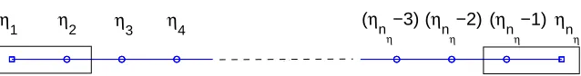
At the boundary nodes, we compute the first derivative here using special compact local stencils (Figure 3). These proposed stencils are constructed as follows. Consider a boundary nodeη1. Its associated stencil is [η1,η2]. The conversion system of this stencil is presented as the following matrix-vector multiplication   u1 u2 du2 dη  = H_sp H_sp

| {z } C_sp 1     w1 w2 c1 c2   

, (36)

whereC_sp

1 is the conversion matrix; andHsp,Hspmatrices defined as

H_sp=

H1(η1) H2(η1) η1 1 H1(η2) H2(η2) η2 1

, (37)

H_{sp= H1(}η2_{) H2(}η2_{) 1 0 . (38)}

Solving (36) yields

    w1 w2 c1 c2    =Csp−11

  u1 u2 du2 dη 

The boundary value of the first-order derivative of u is thus obtained by substituting (39) into (25) and takingη=η1

du(η1)

dη =

H1(η1) H2(η1) 1 0

C−1

sp1

u1 u2 du_dη2

T

, (40)

or dun₁

dη −

dφsp3(η1) dη

dun₂ dη =

dφsp1(η1) dη u

n 1+

dφsp2(η1) dη u

n

2, (41)

where_{φspi(η)}

3

i=1is the set of IRBFs in the physical space. We rewrite equation (41) in matrix-vector form

h

1 ₋dφsp3_dη(η1)

i" dun

1 dη dun2 dη

#

=h dφsp1(η1) dη

dφ_sp2(η1) dη

i _un 1 un₂

. (42)

In a similar manner, one can calculate the first derivative of u at the other boundary nodeηn_η.

The IRBF system on a grid line for the first derivative of u is obtained by letting the interior node taking value from 2 to(nη−1)in (35) and making use of (42),

L_ηubn_{η =}A_ηubn_{. (43)}

3.2.2 Second-order derivative compact approximations

To approximate nodal values of the second-order derivative, we represent the conversion system of the present compact stencil as a matrix-vector multiplication

       u1 u2 u3 d2u1 dη2 d2u3 dη2

       = H G

| {z } C₂      

w′₁ w′₂ w′₃ c′₁ c′₂

    

, (44)

where ui=u(ηi) (i_{∈ {}1,2,3_}); d2ui

dη2 = d2_u

dη2(ηi) (i∈ {1,3});C2the conversion matrix; and H,G sub-matrices defined as (28) and

G ₌

G1(η1) G2(η1) G3(η1) 0 0 G1(η3) G2(η3) G3(η3) 0 0

,respectively. (45)

Solving (44) yields

     

w′₁ w′₂ w′₃ c′₁ c′₂

     =

C−1

2        u1 u2 u3 d2_u 1 dη2 d2_u 3 dη2

which maps the vector of nodal values of the function and of its second-order derivative to the vector of RBF coefficients including the two integration constants. Approximate expression for the second-order derivative in the physical space is obtained by substituting (46) into (24)

d2u(η)

dη2 =

G1(η) G2(η) G3(η) 0 0

C−1

2

b

u

dd2_u dη2

!

, (47)

whereη1_≤η_≤η3;u_b= (u1,u2,u3)T; anddd 2_u dη2 =

d2_u 1 dη2,

d2_u 3 dη2

T

. It can be rewritten in the form

d2u(η)

dη2 = 3

∑

i=1

d2ϕi(η)

dη2 ui+

d2ϕ4(η)

dη2 d2u1

dη2 +

d2ϕ5(η)

dη2 d2u3

dη2, (48)

or

d2un(η)

dη2 = 3

∑

i=1

d2ϕi(η)

dη2 u n i +

d2ϕ4(η)

dη2 d2_un

1 dη2 +

d2ϕ5(η)

dη2 d2un₃

dη2, (49)

where{ϕi(η)_}5

i=1is the set of IRBFs in the physical space.

Collocating (49) at the central node of the compact stencil, i.e.η=η2, leads to

−d

2ϕ4₍η2₎

dη2

d2un₁ dη2 +

d2un₂ dη2 −

d2ϕ5(η2)

dη2

d2un₃ dη2 =

d2ϕ1(η2)

dη2 u n 1+

d2ϕ2(η2)

dη2 u n 2+

d2ϕ3(η2)

dη2 u n 3, (50)

or in matrix-vector form

h

−d2ϕ4(η2)

dη2 1 −

d2_ϕ 5(η2) dη2

i    

d2_un

1 dη2 d2_un

2 dη2 d2un3 dη2

   =

h

d2_ϕ 1(η2) dη2

d2_ϕ 2(η2) dη2

d2_ϕ 3(η2) dη2

i 

un₁ un₂ un₃



. (51)

At the boundary nodes, we compute the second derivative here using special compact local stencils (Figure 3). Consider a boundary node, e.g.,η1. The conversion system of its associated 2-node stencil is presented as the following matrix-vector multiplication

  

u1 u2 d2u2 dη2

  = H_sp G_sp

| {z } C_sp 2     w1 w2 c1 c2   

whereC_sp

2 is the conversion matrix;Hspdefined as before; and

G_{sp= G1(}η2_{) G2(}η2_{) 0 0 . (53)}

Solving (52) yields

    w1 w2 c1 c2    =Csp−12

  

u1 u2 d2_u 2 dη2

 

. (54)

The boundary value of the second-order derivative of u is thus obtained by substituting (54) into (24) and takingη=η1

d2_u(η1₎ dη2 =

G1(η1) G2(η1) 0 0

C−1

sp2

u1 u2 d 2_u

2 dη2

T

, (55)

or d2un₁

dη2 −

d2ϕsp3(η1) dη2

d2un₂ dη2 =

d2ϕsp1(η1) dη2 u

n 1+

d2ϕsp2(η1) dη2 u

n

2, (56)

where{ϕspi(η)}

3

i=1 is the set of IRBFs in the physical space. We rewrite equation (56) in matrix-vector form

h

1 ₋d 2_ϕ

sp3(η1) dη2

i 

d2un₁ dη2 d2un2 dη2



=h d2ϕsp1(η1) dη2

d2_ϕ

sp2(η1) dη2

i _un 1 un₂

. (57)

The IRBF system on a grid line for the second derivative of u is obtained by letting the interior node taking value from 2 to(n_η−1)in (51) and making use of (57),

L_ηηbun_ηη=B_ηηubn_{, (58)}

whereL_ηη,B_{ηη are nη×nη matrices.}

3.3 Temporal discretisation

The temporal discretisation of (1)-(3) using the Adams-Bashforth scheme [Butcher (2003)] for the con-vection term and the Crank-Nicolson scheme [Crank and Nicolson (1996)] for the diffusion term yields

∇.un=0, (59)

un₋un−1 ∆t +

3 2(u

n−1_.∇)un−1₋1 2(u

n−2_.∇)un−2

=

−∇pn−1/2+1

2

r

Pr Ra ∇

2_un_+∇2_un−1_+fn−1/2

b +f

n−1/2

Tn₋Tn−1 ∆t +

3 2(u

n−1_.∇)Tn−1

−1₂(un−2.∇)Tn−2

=

1 2√PrRa ∇

2_Tn_+∇2_Tn−1_+fn−1/2

I,T . (61)

We apply the pressure-free projection/fractional-step method developed in Kim and Moin (1985) to solve (60). This equation is advanced in time according to the following two step procedure

u∗,n₋un−1

∆t +

3 2(u

n₋1_.∇)un₋1

−1₂(un−2.∇)un−2

=

1 2

r

Pr Ra ∇

2_u∗,n_+∇2_un−1_+fn−1/2

b +f

n−1/2

I , (62)

un−u∗,n

∆t =−∇φ

n_{, (63)}

where u∗= (u∗,v∗)Tdenotes the intermediate velocity vector; andφthe pseudo-pressure. It is noted that u∗,ndoes not satisfy the continuity equation (59) and the actual pressure p is derived as

pn−1/2=φn₋ ∆t

2

r

Pr Ra

!

∇2_φn_{. (64)}

3.4 Algorithm of the computational procedure

• Step 0: Start with the given initial and boundary conditions. In this study, the initial conditions are zero for the velocity and temperature fields.

• Step 1: Compute thermal Eulerian counterpartetn, using a formula similar to (15), which is then transferred to Lagrangian nodes to obtainTenusing a formula similar to (19).

• Step 2: Compute F_I,Tn−1/2, using a formula similar to (17), which is then transferred to Eulerian nodes to obtain f_I,Tn−1/2using a formula similar to (20).

• Step 3: Solve (61) for the solution Tnwith known f_I,Tn−1/2and prescribed boundary condition T_Γn. • Step 4: Compute the body force fn_b−1/2from the temperature field as

fn_b−1/2=0,Tn−1/2T =

0,T

n_+Tn−1

2

T

. (65)

• Step 6: Compute Fn_I−1/2from (17), which is then transferred to Eulerian nodes to obtain fn_I−1/2via (20).

• Step 7: Solve (62) for u∗,nsubject to the following boundary condition [Kim and Moin (1985)]

u∗,n_|Γ=un_b+∆t ∇φn−1_|Γ. (66)

For a more efficient solution, one can apply the alternating direction implicit (ADI) algorithm to solve (62) and (61) as shown in Thai-Quang, Mai-Duy, Tran, and Tran-Cong (2012).

• Step 8: Equations (63) and (59) are then solved in a coupled manner for unand φn in which the boundary condition for the pseudo-pressure φ is not required. The values ofφn are obtained for the interior nodes only. After that, the values ofφ at the boundary nodes are extrapolated from known values at the interior nodes and known Neumann boundary values derived from (63) (i.e., ∇φn_{|Γ= u}∗,n

b −unb

/∆t) [Thai-Quang, Le-Cao, Mai-Duy, and Tran-Cong (2012)]:

_φn 1,j φn nx,j =

H1(x1,j) ··· Hnx(x1,j) x1,j 1

H1(xnx,j) ··· Hnx(xnx,j) xnx,j 1         

H1(x2,j) ··· Hnx(x2,j) x2,j 1

H1(x3,j) ··· Hnx(x3,j) x3,j 1

..

. . .. ... ... ...

H1(xnx−1,j) ··· Hnx(xnx−1,j) xnx−1,j 1

H1(x1,j) ··· Hnx(x1,j) 1 0

H1(xnx,j) ··· Hnx(xnx,j) 1 0         

−1

         φn 2,j φn 3,j .. . φn

nx−1,j

∂φn 1,j/∂x ∂φn

nx,j/∂x           , (67)

for a x-grid line, and φn i,1 φn i,ny ! =

H1(yi,1) ··· Hny(yi,1) yi,1 1

H1(yi,ny) ··· Hny(yi,ny) yi,ny 1         

H1(yi,2) ··· Hny(yi,2) yi,2 1

H1(yi,3) ··· Hny(yi,3) yi,3 1

..

. . .. ... ... ...

H1(yi,ny−1) ··· Hny(yi,ny−1) yi,ny−1 1

H1(yi,1) ··· Hny(yi,1) 1 0

H1(yi,ny) ··· Hny(yi,ny) 1 0         

−1

         φn i,2 φn i,3 .. . φn

i,ny−1

∂φn i,1/∂y ∂φn

i,ny/∂y           , (68)

for a y-grid line. It is noted that for flows with irregular outer boundaries, instead of solving (63) and (59), we solve (59)-(60) simultaneously for unand pn−1/2in which pn−1/2involves the interior nodes only (the boundary condition for pn−1/2is not required here).

4 Numerical examples

It has generally been accepted that, among RBFs, the multiquadric (MQ) function tends to result in the most accurate approximation [Franke (1982)]. We choose MQ as the basis function in the present calculations

Gi(x) =

q

(x₋ci)T(x−ci) +a2i, (69)

where x= (x,y)T _{is the position vector of the point of interest; and c}

i = (xci,yci)

T _{and a}

i the position vector of the centre and the width of the ith MQ, respectively. For each stencil, the set of nodal points is taken to be the set of MQ centres. We simply choose the MQ width as ai=βhiin whichβ is a given positive number and hi the distance between the ith node and its nearest neighbouring node. For the calculations in this paper,β =25 andβ =50 are employed. We assess the performance of the present scheme through following measures:

• the root mean square (RMS) error defined as

RMS= s

∑N

i=1(ui−ui)2

N , (70)

where N is the number of nodes over the whole domain; and u the analytic solution,

• maximum absolute error (L∞) defined as L_∞=max

i |ui−ui|, (71)

• the error behaviour, expressed as O(hα), where h is an average grid size; andαthe average rate of grid convergence, determined in the least square sense,

• the convergence measure based on the velocity magnitude (CMvel) in the whole analysis domain is defined as (given two successive grids)

CMvel=

r

∑N i=1

vel_ict f g−vel_if g

2

r

∑N i=1

vel_if g

2 , (72)

A flow is considered to reach a steady state when

s

∑N

i=1(uni −u n−1 i )2

N <10

−9_{, (73)}

where un_{and u}n−1_{are the approximate solutions at the current and previous time levels, respectively.} Since the approximations are presently based on RBFs, distances between two neighbouring nodes in the stencil can be different. This capability is exploited here to handle non-rectangular outer boundaries in a direct manner (i.e. body-fitted grid). We can thus retain a body-conforming treatment for rectangular and non-rectangular outer boundaries. We numerically demonstrate this ability with the following example

∂2_u ∂x2 +

∂2_u

∂y2 =−8π

2_{sin(2πx)sin(2πy), (74)}

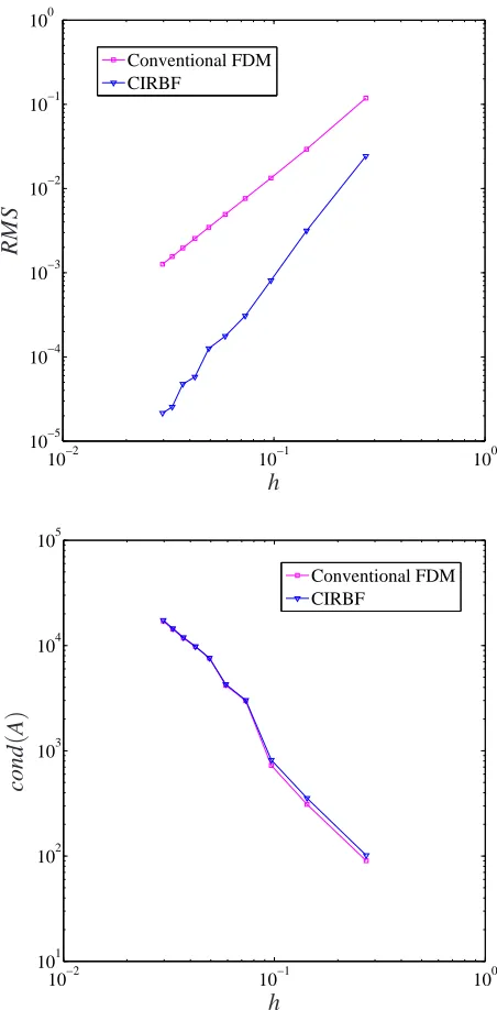
defined on a circular domain of radius R=1.5 and subject to Dirichlet boundary condition. Its exact solution is u=sin(2πx)sin(2πy). A number of grids, namely_{12_×12, 22_×22, . . . , 102_×102_}, are employed to study the grid-convergence behaviour of the solution (Figure 4). Those interior nodes that fall very close to the boundary (within a distance of h/8) are removed from the set of of nodal points. Figure 5 shows the matrix condition number and the RMS error of the interior solution against grid size. Results by the Cartesian-grid finite-difference method (FDM) [Sanmiguel-Rojas, Ortega-Casanova, del Pino, and Fernandez-Feria (2005)] are also included for comparison purposes. The solution converges as O(h2.03)for FDM and quite fast as O(h3.17)for the present method. The two methods have similar condition numbers of the system matrix.

4.1 Taylor-Green vortices

This problem is taken from Uhlmann (2005), where the analytic solution is given by

u(x,y,t) =sin(πx)cos(πy)e−2π2t/Re, (75)

v(x,y,t) =₋sin(πy)cos(πx)e−2π2t/Re, (76) p(x,y,t) =0.5 cos2(πy)₋sin2(πx)e−4π2t/Re, (77) from which one can derive the initial solution, the dependent boundary conditions and the time-dependent desired velocities U(d)on the inner immersed boundaries. The solution is computed at Re=5 and t=0.3 using a time step∆t=0.001 andβ=25 for the following two domains

4.1.1 Circular domain

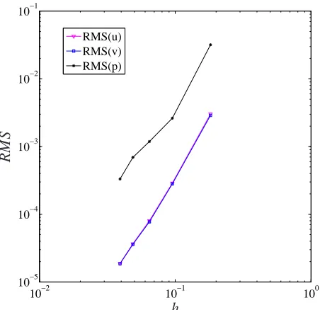
grid size h. The solutions converge as O(h3.31), O(h3.29)and O(h2.87)for the x-component velocity, y-component velocity and pressure, respectively. It can be seen that fast rates of convergence (about third order) are achieved with the present method. Figure 7 shows the analytic and computed vorticity isolines using a grid of 52_×52, which are graphically indistinguishable.

4.1.2 Concentric annulus between two circular cylinders

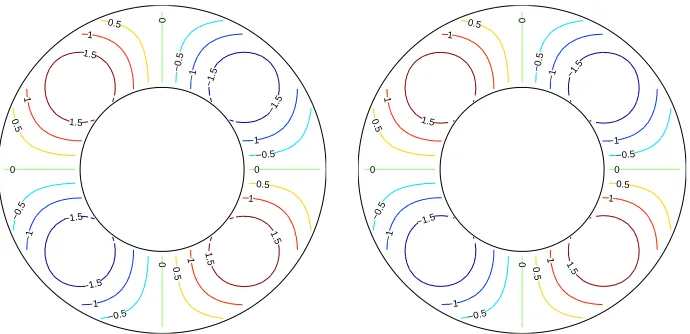
The outer and inner radii of this domain are taken as Ro=1 and Ri =0.5, respectively. We employ a set of grids, namely_{22_×22,32_×32, . . . , 52_×52_}to represent the problem domain. Figure 8 shows the Eulerian nodes distributed inside and on the outer boundary, and Lagrangian nodes distributed on the inner boundary, for instance, by a grid of 22_×22. Figure 9 shows the analytic and computed vorticity isolines using a grid of 52_×52, where an excellent agreement can be seen. The L_∞errors of the velocity components and pressure against the grid size h are presented in Figure 10. The solutions converge as O(h2.02), O(h2.03)and O(h2.02)for u, v and p, respectively. The rates of convergence are reduced due to the effect of using regularisedδh functions, which are second-order accurate [Uhlmann (2005)], in the IB approach.

4.2 Rotational flow

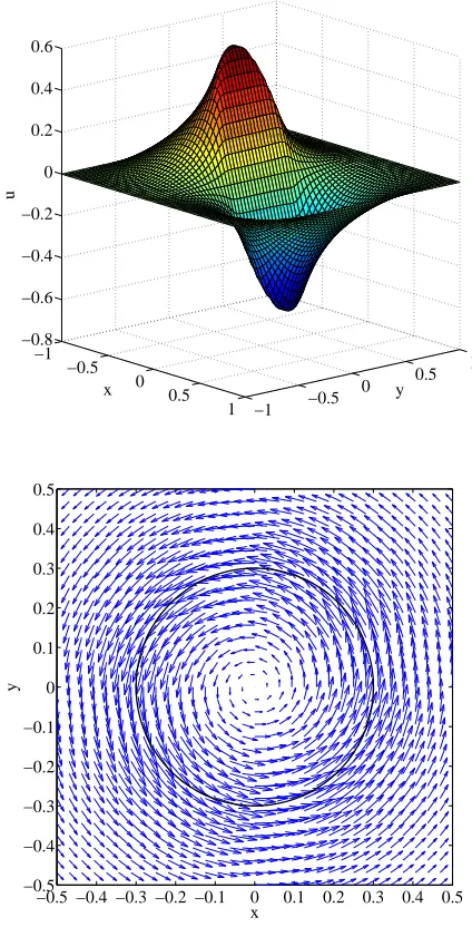
The present scheme is further verified with a rotational flow, where a circular ring (zero thickness) of R=0.3 is embedded in a square domainΩ= [₋1,1]_×[₋1,1]. The solid ring rotates about its centre with an angular velocity ω=2. The simulation is conducted for Re=18 using a grid of 65_×65 and ∆t=h/4 as in Le, Khoo, and Peraire (2006). Plots of the velocity u and velocity vector in a subdomain

[₋0.5,0.5]_×[₋0.5,0.5] at t=10 are shown in Figure 11, in which the flow behaviours observed here are very similar to those reported in Le, Khoo, and Peraire (2006).

4.3 Lid-driven cavity flow with multiple solid bodies

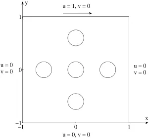
This test problem is concerned with the lid-driven cavity flow in a square domainΩ= [₋1,1]_×[₋1,1]

containing five fixed rigid circular cylinders (Figure 12). The radius of the cylinders is R=0.15 and their centres are located at(0,0),(0,₋0.6),(₋0.6,0),(0,0.6)and(0.6,0), respectively. The top wall is driven from left to right by a unit velocity whereas the other walls are stationary. The Lagrangian nodes are distributed on the boundaries with a grid spacing ratio∆s/h=0.85. These parameters are taken from Su and Lai (2007).

4.4 Flow between a rotating circular and a fixed square cylinder

Consider a flow in a concentric annulus between a square cylinderΩ= [₋2,2]_×[₋2,2]and a circular cylinder of R=1 (Figure 15). The inner cylinder rotates with an angular velocityω=1 while the outer cylinder is stationary. This problem is taken from Lewis (1979). The boundary conditions are as follows

u=0 on x=_±2, y=_±2, (78)

u=−ωy,v=ωx on R=1. (79)

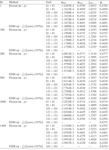
The calculations are carried out on a set of uniform grid N_{∈ {}61_×61,81_×81,101_×101,121_×121,131_× 131,141_×141_} and a set of time step∆t_{∈ {}0.001,0.0005,0.00025,0.0001_} for various values of the Reynolds number, namely Re∈ {1, 100, 200, 500, 1000, 1400}. Smaller time step is utilised for denser grid and higher Reynolds number. The maximum values of the stream function and vorticity (ψmax and ζmax), the values of the stream function on the circular cylinder (ψc) and minimum values of the stream function (ψmin) are presented in Table 1. The present results, convergent at a grid of 131_×131, agree well with those reported in Lewis (1979) using a 161_×161 grid.

The streamlines of the flow field using a grid of 131_×131 is shown in Figure 16, in which the vortices at the corners are well captured and in agreement with the results of Lewis (1979).

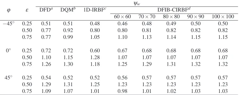
4.5 Natural convection in an eccentric annulus between two circular cylinders

The geometry of this problem can be defined through the following parameters: the eccentricity ε, an-gular position ϕ, radius of the outer cylinder Ro and radius of the inner cylinder Ri (Figure 17). The inner and outer cylinders are heated (Th=1) and cooled(Tc=0), respectively. Calculation is carried out for Pr=0.71, Ro/Ri=2.6 and Ra=104using a set of uniform grids, namely{60×60,70×70,80× 80,90×90,100×100}and a set of time steps∆t∈ {0.001,0.0005,0.00025,0.0001}. Smaller time steps are used for higher grid densities. A distribution of nodes and the boundary conditions are shown in Figure 17.

For symmetrical flows, where the centres of the inner and outer cylinders lie on the vertical symmetrical axis, several values of eccentricity, namely ε _{∈ {}0.25,0.50,0.75,0.95_} and angular direction, namely ϕ∈ {−90◦,90◦_}are considered. Table 2 compares the maximum value of the stream function (ψmax) between the present scheme, one-dimensional integrated radial basis function (1D-IRBF) scheme [Le-Cao, Mai-Duy, and Tran-Cong (2011)] and differential quadrature method (DQM) [Shu, Yao, Yeo, and Zhu (2002)]. It can be seen that good agreement is achieved. The present solutions are convergent at the grid of 90_×90.

DQM [Shu, Yao, Yeo, and Zhu (2002)] and domain-free discretisation method (DFD) [Shu and Wu (2002)]. It is noted that the present governing equations (1)-(3) are different from those used in Shu, Yao, Yeo, and Zhu (2002) and Shu and Wu (2002) by a factor√PrRa. Therefore, to facilitate a comparison, our results in the table, which are computed in the average sense from the values ofψ at the Lagrangian nodes, are multiplied by this factor. The present solutions are convergent at the grid of 90×90.

Figures 18-19 and Figures 20-22 show the isotherms and streamlines of the flow for symmetrical and unsymmetrical flows, respectively, where several combinations of eccentricity and angular direction are considered. Each plot contains 22 contour lines whose levels vary linearly from the minimum to maxi-mum values. All plots look very feasible when compared with those obtained by the 1D-IRBF scheme [Le-Cao, Mai-Duy, and Tran-Cong (2011)], DQM [Shu, Yao, Yeo, and Zhu (2002)] and (DFD) [Shu and Wu (2002)].

5 Concluding remarks

In this paper, we introduce compact integrated RBF approximations into the immersed boundary and point-collocation framework to simulate viscous flows in two dimensions. The direct forcing immersed boundary method is utilised for the handling of inner boundaries, while high-order approximation schemes (Adams-Bashforth/Crank-Nicolson and compact 3-point IRBFs) are employed to represent temporal and spatial derivatives. The proposed method is verified successfully in a series of fluid flow problems in multiply-connected domains. Very good results are obtained using relatively coarse Cartesian grids.

Acknowledgement: Thai-Quang would like to thank USQ, FoES and CESRC for a postgraduate re-search scholarship. This work was supported by the Australian Rere-search Council.

References

Botella, O.; Peyret, R. (1998): Benchmark spectral results on the lid-driven cavity flow. Computers & Fluids, vol. 27, no. 4, pp. 421–433.

Butcher, J. C. (2003): Numerical Methods for Ordinary Differential Equations. John Wiley.

Crank, J.; Nicolson, P. (1996): A practical method for numerical evaluation of solutions of partial differential equations of the heat-conduction type. Advances in Computational Mathematics, vol. 6, no. 1, pp. 207–226.

Ding, H.; Shu, C.; Yeo, K.; Xu, D. (2006): Numerical computation of three-dimensional incompress-ible viscous flows in the primitive variable form by local multiquadric differential quadrature method. Computer Methods in Applied Mechanics and Engineering, vol. 195, no. 7-8, pp. 516–533.

Fadlun, E. A.; Verzicco, R.; Orlandi, P.; Mohd-Yusof, J. (2000): Combined immersed-boundary finite-difference methods for three-dimensional complex flow simulations. Journal of Computational Physics, vol. 161, no. 1, pp. 35–60.

Franke, R. (1982): Scattered data interpolation: Tests of some method. Mathematics of Computation, vol. 38, pp. 181–200.

Goldstein, D.; Handler, R.; Sirovich, L. (1993): Modeling a no-slip flow boundary with an external force field. Journal of Computational Physics, vol. 105, no. 2, pp. 354–366.

Ji, C.; Munjiza, A.; Williams, J. (2012): A novel iterative direct-forcing immersed boundary method and its finite volume applications. Journal of Computational Physics, vol. 231, no. 4, pp. 1797–1821.

Kansa, E. J. (1990): Multiquadrics- A scattered data approximation scheme with applications to computational fluid-dynamics-I. surface approximations and partial derivative estimates. Computers and Mathematics with Applications, vol. 19, no. 8/9, pp. 127–145.

Kim, J.; Kim, D.; Choi, H. (2001): An immersed-boundary finite-volume method for simulations of flow in complex geometries. Journal of Computational Physics, vol. 171, no. 1, pp. 132–150.

Kim, J.; Moin, P. (1985): Application of a fractional-step method to incompressible navier-stokes equations. Journal of Computational Physics, vol. 59, no. 2, pp. 308–323.

Le, D. V.; Khoo, B. C.; Peraire, J. (2006): An immersed interface method for viscous incompressible flows involving rigid and flexible boundaries. Journal of Computational Physics, vol. 220, no. 1, pp. 109–138.

Le-Cao, K.; Mai-Duy, N.; Tran-Cong, T. (2009): An effective integrated-RBFN Cartesian-grid discretization for the stream function-vorticity-temperature formulation in nonrectangular domains. Nu-merical Heat Transfer, Part B: Fundamentals, vol. 55, no. 6, pp. 480–502.

Le-Cao, K.; Mai-Duy, N.; Tran-Cong, T. (2011): Numerical study of stream-function formulation governing flows in multiply-connected domains by integrated rbfs and cartesian grids. Computers & Fluids, vol. 44, no. 1, pp. 32–42.

Leveque, R. J.; Li, Z. (1994): The immersed interface method for elliptic equations with discontinuous coefficients and singular sources. SIAM Journal on Numerical Analysis, vol. 31, no. 4, pp. 1019–1044.

Lewis, E. (1979): Steady flow between a rotating circular cylinder and fixed square cylinder. Journal of Fluid Mechanics, vol. 95, pp. 497–513.

Mai-Duy, N.; Tanner, R. I. (2007): A collocation method based on one-dimensional rbf interpolation scheme for solving pdes. International Journal of Numerical Methods for Heat & Fluid Flow, vol. 17, no. 2, pp. 165–186.

Mai-Duy, N.; Tran-Cong, T. (2001): Numerical solution of differential equations using multiquadric radial basic function networks. Neural Networks, vol. 14, pp. 185–199.

Mai-Duy, N.; Tran-Cong, T. (2001): Numerical solution of Navier-Stokes equations using multi-quadric radial basis function networks. International Journal for Numerical Methods in Fluids, vol. 37, no. 1, pp. 65–86.

Mai-Duy, N.; Tran-Cong, T. (2008): Integrated radial-basis-function networks for computing newto-nian and non-newtonewto-nian fluid flows. Computers & Structures, vol. 87, no. 11-12, pp. 642–650.

Mai-Duy, N.; Tran-Cong, T. (2011): Compact local integrated-rbf approximations for second-order elliptic differential problems. Journal of Computational Physics, vol. 230, no. 12, pp. 4772–4794. Mai-Duy, N.; Tran-Cong, T. (2013): A compact five-point stencil based on integrated rbfs for 2d second-order differential problems. Journal of Computational Physics, vol. 235, pp. 302–321.

Mittal, R.; Iaccarino, G. (2005): Immersed boundary methods. Annual Review of Fluid Mechanics, vol. 37, no. 1, pp. 239–261.

Peskin, C. S. (1977): Numerical analysis of blood flow in the heart. Journal of Computational Physis, vol. 25, pp. 220–252.

Peskin, C. S. (2002): The immersed boundary method. Acta Numerica, vol. 11, pp. 479–517.

Roma, A. M.; Peskin, C. S.; Berger, M. J. (1999): An adaptive version of the immersed boundary method. Journal of Computational Physics, vol. 153, no. 2, pp. 509–534.

Saiki, E. M.; Biringen, S. (1996): Numerical simulation of a cylinder in uniform flow: Application of a virtual boundary method. Journal of Computational Physics, vol. 123, no. 2, pp. 450–465.

Sanmiguel-Rojas, E.; Ortega-Casanova, J.; del Pino, C.; Fernandez-Feria, R. (2005): A cartesian grid finite-difference method for 2d incompressible viscous flows in irregular geometries. Journal of Computational Physics, vol. 204, no. 1, pp. 302–318.

Shu, C.; Wu, Y. L. (2002): Domain-free discretization method for doubly connected domain and its application to simulate natural convection in eccentric annuli. Computer Methods in Applied Mechanics and Engineering, vol. 191, no. 17-18, pp. 1827–1841.

Su, S.-W.; Lai, M.-C. (2007): An immersed boundary technique for simulating complex flows with rigid boundary. Computers & Fluids, vol. 36, no. 2, pp. 313–324.

Thai-Quang, N.; Le-Cao, K.; Mai-Duy, N.; Tran-Cong, T. (2012): A high-order compact local integrated-rbf scheme for steady-state incompressible viscous flows in the primitive variables. CMES: Computer Modeling in Engineering & Sciences, vol. 84, no. 6, pp. 528–558.

Thai-Quang, N.; Mai-Duy, N.; Tran, C.-D.; Tran-Cong, T. (2012): High-order alternating direc-tion implicit method based on compact integrated-rbf approximadirec-tions for unsteady/steady convecdirec-tion- convection-diffusion equations. CMES: Computer Modeling in Engineering & Sciences, vol. 89, no. 3, pp. 189–220.

Tian, Z.; Liang, X.; Yu, P. (2011): A higher order compact finite difference algorithm for solving the incompressible navier-stokes equations. International Journal for Numerical Methods in Fluids, vol. 88, pp. 511–532.

Uhlmann, M. (2005): An immersed boundary method with direct forcing for the simulation of partic-ulate flows. Journal of Computational Physics, vol. 209, no. 2, pp. 448 – 476.

Table 1: Flow between rotating circular and fixed square cylinders: Maximum values of the stream function (ψmax) and vorticity (ζmax), and values of the stream function on the circular cylinder (ψc) by the present method and FDM.

Re Method Grid ψmin ψmax ζmax ψc

1 Present (u₋p) 61_×61 -1.4203E-4 0.4785 1.0472 0.4785

81_×81 -1.3415E-4 0.4699 1.0233 0.4699

101_×101 -1.3588E-4 0.4712 1.0325 0.4712

121_×121 -1.3523E-4 0.4701 1.0249 0.4701

131_×131 -1.3478E-4 0.4695 1.0216 0.4695

141_×141 -1.3472E-4 0.4691 1.0209 0.4691

FDM (ψ₋ζ) [Lewis (1979)] 161_×161 -1.4000E-4 0.4656 1.0186 0.4656

100 Present (u₋p) 61_×61 -1.2527E-3 0.4808 1.2433 0.4808

81_×81 -1.1994E-3 0.4747 1.2374 0.4747

101_×101 -1.1830E-3 0.4711 1.2265 0.4711

121_×121 -1.1788E-3 0.4679 1.2216 0.4679

131_×131 -1.1760E-3 0.4658 1.2198 0.4658

141_×141 -1.1758E-3 0.4652 1.2193 0.4652

FDM (ψ₋ζ) [Lewis (1979)] 161_×161 — — — 0.4577

200 Present (u₋p) 61_×61 -2.0812E-3 0.4777 1.3110 0.4777

81_×81 -1.9988E-3 0.4715 1.3095 0.4715

101_×101 -1.9882E-3 0.4678 1.2992 0.4678

121_×121 -1.9796E-3 0.4652 1.2916 0.4652

131_×131 -1.9721E-3 0.4629 1.2897 0.4629

141_×141 -1.9716E-3 0.4625 1.2893 0.4625

FDM (ψ₋ζ) [Lewis (1979)] 161_×161 — 0.4539 1.2559 0.4539

500 Present (u₋p) 61_×61 -3.0170E-3 0.4738 1.3957 0.4738

81_×81 -2.9114E-3 0.4676 1.4143 0.4676

101_×101 -2.8354E-3 0.4599 1.3732 0.4599

121_×121 -2.7762E-3 0.4526 1.3719 0.4526

131_×131 -2.7298E-3 0.4512 1.3708 0.4512

141_×141 -2.7291E-3 0.4511 1.3702 0.4511

FDM (ψ₋ζ) [Lewis (1979)] 161_×161 -2.7100E-3 0.4465 1.3430 0.4465

1000 Present (u₋p) 61_×61 -3.2525E-3 0.4714 1.4321 0.4714

81_×81 -3.1714E-3 0.4648 1.4899 0.4648

101_×101 -3.1014E-3 0.4502 1.4264 0.4502

121_×121 -3.0326E-3 0.4429 1.3925 0.4429

131_×131 -3.0048E-3 0.4397 1.3767 0.4397

141_×141 -3.0042E-3 0.4394 1.3761 0.4394

FDM (ψ₋ζ) [Lewis (1979)] 161_×161 — — — 0.4375

1400 Present (u₋p) 61_×61 -3.2105E-3 0.4707 1.4329 0.4707

81_×81 -3.1543E-3 0.4637 1.5223 0.4637

101_×101 -3.0785E-3 0.4461 1.4279 0.4461

121_×121 -3.0241E-3 0.4379 1.4117 0.4379

131_×131 -2.9953E-3 0.4324 1.4026 0.4324

141_×141 -2.9947E-3 0.4320 1.4024 0.4320

Table 2: Natural convection in eccentric circular-circular annulus, symmetrical flows: the maximum values of the stream function (ψmax) for two special cases ϕ _{∈ {−}90◦,90◦_} by the present and some other numerical schemes.

ψmax

ϕ ε DQMa 1D-IRBFb DFIB-CIRBFc

60_×60 70_×70 80_×80 90_×90 100_×100

−90◦ 0.25 15.50 15.71 15.26 15.30 15.35 15.36 15.36

0.50 18.32 18.50 18.10 18.39 18.44 18.47 18.47

0.75 20.62 20.72 20.10 20.41 20.47 20.49 20.49

0.95 22.16 22.19 21.91 22.35 22.44 22.49 22.50

90◦ 0.25 11.13 11.26 11.07 11.11 11.13 11.14 11.14

0.50 9.55 9.64 9.51 9.55 9.57 9.58 9.58

0.75 8.12 8.25 8.17 8.18 8.20 8.21 8.21

0.95 7.17 7.28 7.21 7.23 7.24 7.24 7.24

a_{Shu, Yao, Yeo, and Zhu (2002)}

b_{Le-Cao, Mai-Duy, and Tran-Cong (2011)}

c_Present

Table 3: Natural convection in eccentric circular-circular annulus, unsymmetrical flows: the stream function values at the inner cylinders (ψw) for ε _{∈ {}0.25,0.50,0.75_} and ϕ _{∈ {−}45◦,0◦,45◦_} by the present and some other numerical schemes.

ψw

ϕ ε DFDa DQMb 1D-IRBFc DFIB-CIRBFd

60×60 70×70 80×80 90×90 100×100

−45◦ 0.25 0.51 0.51 0.48 0.46 0.48 0.49 0.50 0.50

0.50 0.77 0.92 0.80 0.80 0.81 0.82 0.82 0.82

0.75 0.77 0.99 1.05 1.10 1.13 1.14 1.15 1.15

0◦ 0.25 0.72 0.72 0.60 0.67 0.68 0.68 0.68 0.68

0.50 1.10 1.15 1.28 1.07 1.07 1.07 1.07 1.07

0.75 1.26 1.30 1.18 1.25 1.29 1.31 1.32 1.32

45◦ 0.25 0.54 0.52 0.52 0.56 0.57 0.57 0.57 0.57

0.50 1.29 1.31 1.25 1.23 1.23 1.23 1.23 1.23

0.75 1.09 1.07 1.01 0.98 1.01 1.02 1.03 1.03

a_{Shu and Wu (2002)}

b_{Shu, Yao, Yeo, and Zhu (2002)}

c_{Le-Cao, Mai-Duy, and Tran-Cong (2011)}

Ω

S

2

S

3

S

4

S

1 ∂S

1

∂S

2

∂S

3

∂S

4

Ω

Γ

Figure 1: A schematic outline for the problem domain.

η₁ η₂ η

3

η_n

η

η₁ η₂ η₃ η₄ (η

n

η −3) (η

n

η −2) (η

n

η −1)

Figure 3: Special compact 2-point IRBF stencils for the left and right boundary nodes

10−2 10−1 100 10−5

10−4 10−3 10−2 10−1 100

Conventional FDM CIRBF

h

R

M

S

10−2 10−1 100 101

102 103 104 105

Conventional FDM CIRBF

h

co

n

d

(

A

)

Figure 5: Poisson equation, circular domain,_{12_×12,22_×22, . . . ,102_×102_}: The solution accuracy (top) and the matrix condition number (bottom) against grid size by FDM and the present method. The solution converges as O(h2.03)and O(h3.17)while the matrix condition grows as O(h−2.52)and O(h−2.46)

10−2 10−1 100 10−5

10−4 10−3 10−2 10−1

RMS(u) RMS(v) RMS(p)

h

R

M

S

Figure 6: Taylor-Green vortices, circular domain,_{12_×12,22_×22, . . . ,52_×52_}: The solution accuracy of the velocity components and pressure against grid size. The solution converges as O(h3.31), O(h3.29)

and O(h2.87)for x-component velocity, y-component velocity and pressure, respectively.

−1.5

−1.5

−1

−1

−0.5

−0.5

0

0

0.5

0.5

1

1 1.5

1.5 −1.5

−1.5

−1

−1

−0.5

−0.5

0

0

0.5

0.5

1

1 1.5

1.5

Figure 8: Taylor-Green vortices, concentric annulus: Computational domain and its discretisation (Eule-rian nodes inside the annulus and on the outer boundary, Lagrangian nodes on the inner boundary with a grid of 22_×22).

−1.5

−1.5

−1.5

−1.5

−1

−1

−1

−1

−0.5

−0.5 −0.5

−0.5 0

0

0

0 0.5

0.5

0.5

0.5

1

1

1

1 1.5

1.5

1.5

1.5 −1.5

−1.5

−1

−1

−1

−1

−0.5

−0.5 −0.5

−0.5 0

0

0

0 0.5

0.5

0.5

0.5

1

1

1

1

1.5

1.5

10−2 10−1 10−3

10−2 10−1

L ∞

L_∞(u) L_∞(v) L_∞(p)

h

−1 −0.5

0 0.5

1 −1 −0.5

0 0.5

1 −0.8

−0.6 −0.4 −0.2 0 0.2 0.4 0.6

y x

u

−0.5 −0.4 −0.3 −0.2 −0.1 0 0.1 0.2 0.3 0.4 0.5

−0.5 −0.4 −0.3 −0.2 −0.1 0 0.1 0.2 0.3 0.4 0.5

x

y

−1

0

1

−1

0

1

y

u = 0

v = 0

u = 1, v = 0

u = 0

v = 0

u = 0, v = 0

x

−1 −0.5 0 0.5 1 −1

−0.5 0 0.5 1

x

y

−0.4 −0.2 0 0.2 0.4 0.6 0.8 1 −1

−0.8 −0.6 −0.4 −0.2 0 0.2 0.4 0.6 0.8 1

41×41 61×61 81×81 101×101 121×121

u

y

−2 −1 0 1 2 −2

−1 0 1 2

x y

u = 0, v = 0

u = 0 v = 0 u = 0

v = 0

u = 0, v = 0 R

ω

Re = 1 Re = 100

−0.0001

0 0.001

0.01

0.1

0.3 0.4695

−0.0005

0 0.001

0.01

0.1

0.3 0.4658

Re = 200 Re = 500

0.4629 0.3

0.1

0.010.001 −0.0005 −0.001

0

0.4512 0.3 0.1

0.010.001 −0.001

−0.002

0

Re = 1000 Re = 1400

−0.001

−0.002

0 0.001

0.01

0.1

0.3

0.4397 0.4324

0.3 0.1

0.010.001 −0.001

−0.002

0

ϕ R

i

ε

x y

R o

(x

e, ye)

(0, 0) u=0

v=0 T

c=0

u=0 v=0 T

h=1