Robustness to noise of arterial blood flow estimation methods in CT perfusion

R E S E A R C H A R T I C L E

Open Access

Robustness to noise of arterial blood flow

estimation methods in CT perfusion

Maria Romano

, Michela D

’

Antò

, Paolo Bifulco

, Francesco Fiore

and Mario Cesarelli

Abstract

Background:Perfusion CT is a technology which allows functional evaluation of tissue vascularity. Due to this potential, it is finding increasing utility in oncology. Although since its introduction continuous advances have interested CT technique, some issues have to be still defined, concerning both clinical and technical aspects. In this study, we dealt with the comparison of two widely employed mathematical models (dual input one compartment

model–DOCM - and maximum slope–SM -) analyzing their robustness to the noise.

Methods:We carried out a computer simulation process to quantify effect of noise on the evaluation of an important perfusion parameter (Arterial Blood Flow–BFa) in liver tumours. A total of 4500 liver TAC, corresponding to 3 fixed BFa values, were simulated using different arterial and portal TAC (computed from 5 real CT images) at 10 values of signal to noise ratio (SNR). BFa values were calculated by applying four different algorithms, specifically developed, to these noisy simulated curves. Three algorithms were developed to implement SM (one

semiautomatic, one automatic and one automatic with filtering) and the last for the DOCM method. Results:In all the simulations, DOCM provided the best results, i.e., those with the lowest percentage error compared to the reference value of BFa. Concerning SM, the results are variable. Results obtained with the automatic algorithm with filtering are close to the reference value, but only if SNR is higher than 50. Vice versa, results obtained by means of the semiautomatic algorithm gave, in all simulations, the lowest results with the lowest standard deviation of the percentage error.

Conclusions:Since the use of DOCM is limited by the necessity that portal vein is visible in CT scans, significant restriction for patients’follow-up, we concluded that SM can be reliably employed. However, a proper software has to be used and an estimation of SNR would be carried out.

Keywords:Computed tomography (CT), Liver perfusion, Maximum slope method, Dual-input one-compartment

model, Noise robustness

Background

Quantitative measurements of hepatic perfusion can give important information in detection, assessment and man-agement of various liver diseases. Particular important is the measurement of blood flow within the liver, since changes in tumour vascularisation are significant indica-tors of treatment response of hepatic cancers [1]. Different methods of quantification have been proposed but generally are either invasive or remain controversial [2]. In the last decade, this awareness, the introduction of

multidetector CT systems (MDCT) and the availability of perfusion commercial software have stimulated the clinical interest in perfusion CT technique [3]. This technique consists of sequential acquisitions of images during the intravenous injection of a contrast agent bolus. It provides parameters correlated to tumour vasculature and represents an in vivo marker of tumour angiogenesis [4,5].

Hepatocellular Carcinoma (HCC), the most common malignant liver tumour, is characterized by an increased arterial vascularisation. An accurate assessment of arter-ial perfusion is then crucarter-ial to evaluate HCC response to treatments. Besides, primitive liver tumour diagnosis, as-sessment and staging are critical because PET (Positron * Correspondence:cesarell@unina.it

1_{DIETI, University of Naples,“Federico II”, Naples, Italy} 2

Interuniversity Centre of Bioengineering of the Human Neuromusculoskeletal System, Rome, Italy

Full list of author information is available at the end of the article

emission tomography), that represent the gold standard functional technique, is not a useful tool in the diagnosis and follow up of HCC, because metabolism of glucose in primitive liver tumour is not different from the surround-ing liver parenchima. So, liver perfusion CT studies are increasingly advocated as a means to assess the grade of vascularisation in HCC patients and to evaluate variations in perfusion parameters following locoregional treatments or antiangiogenic drugs. However, although since its introduction continuous advances have interested CT technique, in its use some problems remain still open. They concern both clinical and technical aspects, related, for example, to radiation dose, optimum volume and speed of bolus of contrast material injected, characteristics of the employed CT system and image processing [6-9].

About models to be adopted in assessment of perfu-sion parameters, currently three models are the most used, the maximum slope (SM) method, the dual-input one-compartment model (DOCM) method and the de-convolution method (DC) [8]. The SM method was in-troduced by Miles et al. [10] and, because its underlying principle is relatively simple, it has come to dominate the field of hepatic perfusion measurement. In contrast, this method can underestimate hepatic perfusion, espe-cially portal perfusion, when the “no venous outflow” assumption is violated [11]. This assumption states that washout of contrast medium should not occur prior to the peak time of the initial slope of the tissue time attenu-ation curve (TAC). Thus, a high injection rate of contrast medium is a prerequisite for accurate perfusion measure-ments. To overcome this drawback, a new method of perfusion analysis, the DOCM method, was proposed by Materne et al. [2]. In theory, hepatic perfusion can be estimated correctly with this method regardless of the injection rate. Nevertheless, its use is time-consuming and limited by the necessity to include in the images also the portal vein. Cuenod et al. [12] used a deconvolution tech-nique to evaluate hepatic perfusion. This method provides more robust analysis without a high injection rate, and the estimated perfusion values are theoretically independent from cardiac output, from possible delay of bolus or from other extrahepatic factors such as age or sex [8]. However, the calculation is complex and, mainly, the results are affected by the hemodynamic model used, which makes it unsuitable for the liver [8].

Despite to some encouraging results obtained with these models, there is currently no agreement regarding the optimal analytic method in hepatic CT perfusion and standardization in the use of model is still an open issue.

Recently, different authors [8,13] have dealt with this topic. These studies have shown that no consensus has been reached about the choice of the best model; besides, they do not consider important aspects such as image noise. Noise in perfusion images is related to different

aspects. A greater number of images results in more data points on the time attenuation curve (TAC), and therefore higher reliability of perfusion measurements. Similarly, a larger tube current results in less photon noise within each image. Image noise can also be reduced by using thicker image slices and lower resolution reconstruction filters but at the expense of spatial resolution [3]. Anyway, once the protocol is defined, there is always an unavoid-able amount of noise which could heavily affect perfusion parameters estimation.

In this work, we focused on the comparison of the two most employed mathematical models (DOCM and SM) analyzing their robustness to the noise by means of com-puter simulations; in particular we quantified the effect of noise on evaluation of an important perfusion param-eter (Arterial Blood Flow–BFa) in HCC lesions.

Methods

Patients

Five subjects (4 women and 1 man; age range, 70–77 years; mean, 74.2 years) with multiple or single hypervascular HCC lesions and without cardiac complications were en-rolled for this study, by choosing in our database the images in which portal vein was visible. The diagnosis of HCC tumour was achieved on the basis of AASLD (American Association for the Study of Liver Disease) criteria using established techniques (RM, MDCT and CEUS) or by means of liver biopsy. Other relevant clinical informa-tion and weights were collected for all patients. A target untreated lesion was selected on the basal CTscan (with-out contrast). Then, a perfusion CT study was performed for each patient.

The project was approved by the scientific technical com-mittee of the hospital (National Cancer Institute “Pascale Foundation”, Naples, Italy) as part of an internal research project with note DSC/1957 of 2009 and all patients gave informed consent to undergo investigation.

CT perfusion imaging

Perfusion CT was performed by means of a commer-cially available scanner (Philips Brilliance 16 slices). The perfusion protocol comprised 30 scans (90 kVp, 250 mAs, 4 × 6 mm slice thickness, 1 second gantry rotation time, 3 s acquisition time), which were obtained in correspondence of tumour lesion. A 70 ml bolus of con-trast agent (Iomeron 400 mg/ml) was injected (injection rate 4 ml/s) into an antecubital vein at the beginning of the CT data acquisition. The participants were advised to breathe slowly during the examination to reduce motion artifacts.

Mathematical methods Maximum slope (SM)

The principle of the SM is quite simple, which made it a very attractive method. It is a derivation of Fick principle allowing the separate evaluation of dual liver blood sup-ply component, i.e. arterial blood flow (BFa) and portal blood flow (BFp). BFa is calculated like the maximum slope of the liver TAC in its early phase divided by peak aortic attenuation (Eq.1). The time of peak splenic enhancement is used as cut-off point to separate arterial and portal components. BFp is calculated by dividing the maximum slope of the liver TAC in its late phase (after peak splenic) by peak aortic attenuation [5,11]. Because advanced HCC is practically not nourished by portal blood flow, blood flow in the tumour consists almost exclusively of arterial flow alone [14,15], therefore BFa is here chosen as perfusion parameter. In the following equation (1), Cl(t) is TAC of tumour or liver parenchyma

and Ca(t) is aorta TAC.

BFa¼

dClð Þt

dt max Cað Þt max

ð1Þ

Although its simplicity, the application of this method involves the choice of different processing techniques. In literature [16-18], different TAC processing have been an-alyzed and different algorithms have been developed for the application of this method but details are generally missing and no consensus has been reached about the most reliable algorithm to compute the maximum slope [16]. In particular, in literature it is not defined a method to identify starting and end points of the up-slope calcula-tion [16].

Dual-input one compartment model (DOCM)

With this method, hepatic perfusion parameters are calculated using all TAC points [19]. When this model is used, the differential equation describing the kinetic behaviour of the contrast agent is [1,2,13]:

dClð Þt

dt ¼k1aCaðt−τaÞ þk1pCp t−τp

−k2Clð Þt

ð2Þ

where Cl(t), Ca(t) and Cp(t) are the concentrations of

contrast agent at timet(TAC in the region of interest– ROI – ) in the liver, hepatic artery and portal vein, respectively.τaandτprepresent the transit time of

con-trast agent respectively from the aorta and portal vein ROI, to the liver ROI. The minus signs beforeτaandτp

occurs because the arrival times of the contrast agent to the liver ROI through the hepatic artery and portal vein are generally delayed compared with those to the aorta and portal vein ROI respectively. The parameters k1a, k1p and k2are the rate constants for the transfers

of the contrast agent from the hepatic artery to the liver, from the portal vein to the liver, and from the liver to the blood.

Curves simulation

In order to compare different BFa estimation methods and to test their robustness to noise, we carried out a computer simulation process.

We computed noise-free Cl(t) starting from equation 2.

To solve this equation, we used the linear least-squares method, according to Murase [1], with the assumption that the initial conditions are zero [1]. Besides, we fixed k1a, k1p and k2 values and used a discrete trapezoids

method for the integration.

Holding the hypothesis that in HCC only the arterial flow contribution is significantly changed, as introduced in the above section“Maximum slope”, values relative to healthy subjects were chosen for k1pand k2(respectively,

0.0133 and 0.0333 [1,13]).

k1a was fixed on the basis of a previous work about

HCC [6] (please, see the next Section).

Ca(t) and Cp(t) were obtained from real perfusion CT,

drawing circular ROI as large as possible on patients’ images.

Finally,τaandτpwere assumed to be equal to zero for

simplicity [13].

In Figure 1 an example of the curves used for the study is shown.

Noise simulation

To investigate the effect of noise on BFa estimation, we added noise to the simulated Cl(t). Specific models of

noise should be adopted for the images here treated, but there is no literature available about this particular topic. Models employed in some research works about perfu-sion or described in other medical applications generally assume the noise to be additive, white and Gaussian [1,13,20]. So, we computed the noise by generating nor-mally distributed random numbers with null mean and unit variance. Nevertheless, short sequences obtained by Matlab noise generator could not have unit variance. In order to ensure the unit variance of the noise, the generated random sequence (for simplicity called rum) was normalised with respect to its standard deviation. Then, in order to obtain set signal to noise ratio (SNR), we multiplied rum by the square root of the ratio between signal power and the set SNR, according to formula 3:

noise¼

ffiffiffiffiffiffiffiffiffiffiffiffiffiffiffiffiffiffiffi

P signalð Þ SNR

r

1

std rumð Þrum ð3Þ

where P(signal) is the power of the simulated Cl(t)

In Figure 2 it is shown an example of a simulated Cl

TAC and the corresponding noisy curve.

In order to obtain curves with different levels of noise, SNR ranged from 10 to 100 (step 10, absolute values). For each SNR value, the noise simulations were repeated thirty times; so that we obtained 300 Clnoisy curves for

each Cl(t).

Simulation study

The procedure described in the previous Section (corre-sponding to 300 simulations with the same Clcurve and

different signal noises, in the following also called patient

study) was reproduced for each of the five patients (using the corresponding real Caand Cpcurves).

Then, the whole simulation study (involving all pa-tients, i.e. 1500 simulations) was repeated three times, with different values of K1a (for a total of 4500

simulations).

In particular, as values for k1a were chosen 0.0146,

0.0096 and 0.0189. They were computed starting from mean, minimum and maximum values of BFa experi-mentally obtained in a previous work [6], making the appropriate change of measurement units and rounding to fourth decimal digit.

Figure 1Example of TAC used for the study.An example of TAC used for this study (patient # 1, internal numbering). Dashed and dotted lines represent respectively aorta and portal TAC obtained from real perfusion images. Black stars mark a Cl(t) (tumour TAC) estimated with the simulation study.

BFa estimation

To use known perfusion units (ml × min−1× 100 ml−1), ac-cording to literature, all perfusion values were multiplied by 60 s/min and by 100 ml (of blood)/ml (of tissue), where we assumed a specific tissue gravity of 1.0 [11].

Experimental BFa values were estimated by applying four different algorithms (described below) to the noisy simulated Cl(t) curves. Three algorithms were developed

to implement SM and the last for the DOCM method. The algorithms performances were evaluated by com-paring the obtained BFa with the set value.

The set BFa values, used as reference in the three simu-lation studies, were 87.6, 57.6 and 113.4 ml/min/100 ml (obtained multiplying by 6000 the k1a values chosen for

the simulations).

SM semiautomatic algorithm

In this version, according to other algorithms proposed in literature [13], the algorithm is based on the manual selection of starting (S) and end (E) points of TAC range on which to compute the maximum slope [21,22]. S and E points can be selected on Cl(t) by the operator through a

simple interface, also developed with Matlab. The max-imum slope was estimated as the slope of the straight line that fits the curve samples, between the two selected points, best in a least-squares sense.

SM automatic algorithm

According to literature [16], the simulated Cl (t) curve

was differentiated and an array (here named 1-D-diff ), which represented the contrast time variations, was com-puted. At this point, the search of the maximum element was limited to the rise portion of the curve; in this case S was set equal to 10 s and E was fixed at one third of Cl

length. Since, as mentioned, there are not references in literature, we based this choice on simulated curves com-puted by Bae [7] and on our experience. The largest elem-ent between S and E in the 1-D-diff array (which of course is positive) corresponds to the maximum contrast vari-ation. Three consecutive data points of Clcurve, centred

around the identified element, were then considered. The three consecutive points were fitted using a linear curve fitting model, the best fitting was again chosen minimizing the square mean error. The slope of the regression line was considered as the maximum slope of the TAC.

SM automatic algorithm with smoothing

In this last version of the algorithm, as proposed in lit-erature [17], we smoothed Cl(t), before automatic

com-putation of maximum slope, in order to reduce noise contribute. For smoothing, we applied an average filter (5th-order moving-average filter, cut-off frequency equal to 0.1 Hz).

DOCM algorithm

In this case, to estimate the kinetic parameters and consequently BFa, we solved the eq. 2 using the same methodology described in the section“Curves simulation” but, of course, leaving the k values unknowns.

Noise estimation

Assuming that the performances of the different signal processing techniques depend on SNR, we implemented a simple procedure for SNR estimation, to be applied on real curves in order to establish if the actual SNR permits the use of the proposed algorithms.

For assessing SNR, we computed the ratio between the estimates of signal power and noise power. In particular, the estimation of signal power was carried out calculating the power of the whole noisy Cl(t) curve.

Then, we estimated noise contribution as power of the curve in its final tract, where it is possible to assume that the contrast enhancement reached an almost steady-state plateau [7]; in this signal tract the computation of noise power is possible simply after removing any possible linear trend of the signal.

Results

For simplicity, in the following, the acronyms listed in Table 1 will be used to indicate the results obtained.

In Figure 3, to provide a clear, visual example of the software functioning, regression lines estimated from the three different algorithms which implement SM are shown superimposed on the simulated noisy Clcurve represented

in Figure 2 (DOCM algorithm is not reported because of

Table 1 Acronyms

Acronym Meaning

BFa_DOCM BFa values computed with the DOC algorithm

BFa_SM_sa BFa values obtained with the SM semiautomatic algorithm

BFa_SM_a BFa values provided by the SM automatic algorithm

BFa_SM_af Results of the SM automatic algorithm with filtering (i.e. after Cl(t) smoothing)

Patient study Simulations carried out for one patient and for all ten SNR values (for a total of 300 simulations)

SNR study Simulations carried out for one SNR value and for all five patients (150 simulations)

Simulation study 1500 simulations (all patients and all SNR values)

BFa min Simulation study (five patients, ten SNR values, thirty simulations, for a total of 1500 simulations) carried out with the reference BFa set at the min value (57.6)

BFa mean Simulation study carried out with the reference BFa set at the mean value (87.6)

BFa max Simulation study carried out with the reference BFa set at the max value (113.4)

course it computes a value of BFa without the necessity of a regression line).

For the simulation shown in Figure 3 (one of the thirty simulations carried out for the patient #1 with SNR = 50 in the simulation study BFa max), BFa computed with DOCM algorithm was 116.90 (very close to the refer-ence BFa) and the estimated SNR was 47.89.

The results obtained in the three simulation studies (different reference BFa values) are reported as mean ± standard deviation in Table 2. Each value of Table 2 was computed considering all five patients. The BFa values obtained in our simulation studies have shown a similar behaviour for all studied patients.

In Figure 4 are shown, as average values, the results of all thirty executions, at different SNR, correspond-ing to the second patient, obtained in the simulation study BFa mean.

Observing Table 2 and Figure 4, it is possible to do some considerations (suitable for each condition – different patient and/or simulation study).

BFa values obtained with DOCM and automatic max-imum slope algorithm with smoothing (columns named BFa_DOCM and BFa_SM_af ) are the closest to the set value; though the automatic algorithm after filtering fails if SNR is at too low levels.

Manual selection of maximum slope (column BFa_ SM_sa) leads always to underestimate BFa values, none-theless results are little variable, as it results more clearly in Figure 4.

Finally, automatic algorithm (without any smoothing processing), because the great effect of the noise on Cl(t),

provided always the worst results (column BFa_SM_a), being the most variable and overestimating the set BFa in each simulation study and for each SNR value.

To better highlight differences between the estimated values of BFa and that set as reference (87.6 in this simulation study), we computed also the relative per-centage errors (formula 4).

E¼100jBFa−BFa refj

BFa ref ð4Þ

where BFa is the computed value and BFa_ref is the reference.

Values obtained for the simulation study with BFa equal to 87.6 are shown in Figure 5, grouped for each SNR study.

Mean and standard deviations of all these errors computed for the three simulation studies (BFa min, BFa mean, BFa max) are reported in Table 3, from which it is clear that the DOCM method on average makes the lowest error.

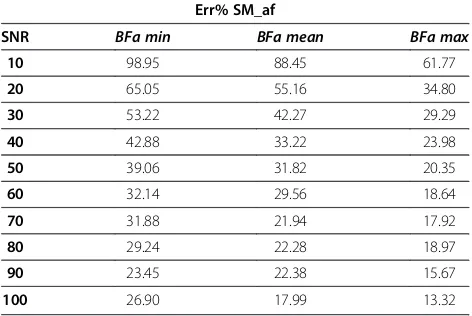
In Table 4, instead, we reported the average value of the relative percentage errors for the automatic algo-rithm with filtering computed for each SNR study, since this parameter affects strongly the performance of this software.

Results reported in Table 4 indicate that the relative percentage error depends both on BFa value and SNR level.

Considering then the semiautomatic algorithm (SM_sa), it is possible to observe (Table 3 and Figure 5) that the standard deviation of % error ois quite low, regardless to SNR.

This result suggested us to compute a “modified” BFa value starting from that estimated with the semiauto-matic algorithm and using a correcting factor (CF), com-puted as the overall mean percentage error, about equal to 35, as in formula 5.

BFamodified ¼100

BFaSM sa

100−CF ð5Þ

In this way, starting from the estimations obtained for the different SNR studies (second, fourth and sixth col-umn in Table 5), we obtained the BFa values reported in (See figure on previous page.)

Figure 3Example of behaviour of the algorithms developed for implementation of slope method.Behaviour of the algorithms developed for implementation of SM. Estimated regression lines are shown superimposed on a simulated noisy Cl curve (the same reported in Figure 2). From the top:a)semiautomatic algorithm, black stars represent start and end points selected from the operator;b)automatic algorithm; c)automatic algorithm after smoothing. In b and c the black stars represent the point automatically recognised from the algorithm as sample at maximum slope. In this case, computed BFa were respectively: 68.55, 78.30 and 123.81 ml/min/100 ml.

Table 2 BFa mean values obtained in the three simulation studies

DOCM SM_sa SM_a SM_af

BFa min (57.6) 58.25 ± 6.71 39.63 ± 6.53 142.53 ± 109.90 78.01 ± 29.31

BFa mean (87.6) 88.69 ± 8.27 58.83 ± 10.53 192.67 ± 149.63 109.23 ± 41.24

BFa max (113.4) 113.66 ± 10.19 67.14 ± 16.70 208.54 ± 153.51 124.17 ± 39.63

Table 6 (third, fifth and seventh column), which are much closer to the reference BFa value.

Finally, concerning SNR estimation, in Table 6 we reported the mean values obtained in the 150 simulations (30 for each patient) performed for each SNR study and for each simulation study.

It is possible to observe that set and estimated values, except in a few cases, are always very similar.

Discussion

Diagnostic imaging techniques provide limited evaluations of tissue characteristics beyond morphology, whereas quantifying reliably angiogenesis is very important for

evaluation of tumour progression and monitoring of the therapeutic response of HCC. CT perfusion has the po-tential to achieve this objective [23,24]. This technique is quickly spreading in the field of hepatic oncology, since it is minimally invasive and can be quite simply incorporated into routinely CT protocols providing precious informa-tion about tumour grade and angiogenesis monitoring

“in vivo”[5-7]. However, consistent, routine clinical ap-plication of perfusion CT requires a reliable employ of the technique. At the moment of research starting, there existed encouraging preliminary findings about repro-ducibility of the methodology and intra- and inter-observer variability but they did not regard the liver

Figure 4BFa mean values (over 30 simulations) computed with BFa reference set to 87.6 (second patient).BFa mean values (second patient) computed with the four algorithms for each set SNR (shown on the x-axis). Reference BFa was 87.6.

[25]. Besides, some aspects of crucial importance are still debated, for example effects of extra-hepatic factors [7] and standardization and validation of the analytic method to be employed [24], problem here faced. More-over, although software packages involving perfusion parameters computation were addressed as advanta-geous in oncological applications [7], details of signal processing are lacking in literature so making difficult the procedures’reproducibility.

Aim of this work was to compare two among the most diffused methods, SM and DOCM, testing three differ-ent algorithms for application of SM and one for DOCM and studying noise effect on the estimation of BFa, since, at the best of our knowledge, no study of this kind is available in literature. In fact, for example, Kanda et al. [8] have recently compared three analytic methods (SM, DOCM and DC, in their work named by different acro-nyms) but without considering noise contribution and Murase et al. [1] investigated effect of noise but only in the comparison of two computation methods for DOCM use.

Since there is no a practical method to evaluate in a reliable and accurate way perfusion parameters in vivo that can be considered the gold standard [11], we carried

out a computer simulation process comparing estimated BFa with reference values.

In this study, according to literature, we considered a SNR range between 10 and 100. The lowest values charac-terise TAC computed using very small ROI or the pixel-by-pixel analysis typical in maps generation.

In all the 4500 simulations (30 for each of the 10 SNR values, 300 for each patient, 1500 for each simulation study), DOCM provided the best results, i.e., those with the lowest percentage error compared to the reference value of BFa (see Table 3).

About SM, its application by means of the semiauto-matic algorithm provided always results lower than both the set BFa value and values estimated with the other methods, as shown in Figure 4. This is not so surprising, in fact other authors highlighted that perfusion parame-ters computed with SM are lower than those obtained with DOCM method, both in clinical studies and in simulation analysis [8,11,13], though, there, technical de-tails about signal processing are not given. Furthermore, it is important to put in evidence that the semiautomatic algorithm computes the linear interpolation of the TAC between two points (start and end points) providing the estimation of its slope, and in turn an estimate of the average slope, while the automatic algorithm estimates the slope of the curve at its maximum slope point (over-estimated in presence of noise). Of course, the mean slope value is surely lower than the maximum slope.

However, results got with the semiautomatic algorithm are quite stable, in the sense that they show a standard deviation of the percentage error (Table 3, column named Err% SM_sa) very low and not dependent on SNR. Hence, we propose to use a correcting factor (for-mula 4) to compute the BFa value starting from that in output of the software. Here, we imposed CF equal to 35 (mean percentage error), obtaining satisfactory results (please refer to Table 5); however, a deepened study, carried out on a more numerous set of images would be useful in order to set this parameter in a more general and reliable way.

Concerning the application of SM with automatic algorithm following a smoothing filtering, obtained re-sults are not so far from the set value, confirming that it is useful to attenuate the irregularities of TAC before assessing perfusion parameters, as reported also in literature [17]. Nevertheless, this is valid only until SNR is over 50 (please refer to Figure 5 and Table 4), beyond this value the percentage error increases up to about 40%. Therefore, in order to apply this algorithm, is necessary to know the SNR of the image under analysis. Since, of course, in clinical practice this value is not known, we proposed a simple procedure for its estima-tion. As shown in Table 6, obtained results are satisfac-tory. So it could be possible to include this procedure in Table 3 Relative percentage errors obtained on average

for each simulation study

Err% DOCM Err% SM_sa Err% SM_a Err% SM_af

BFa min 8.27 ± 8.28 31.39 ± 10.79 182.82 ± 157.19 44.28 ± 43.40

BFa mean 6.74 ± 6.73 33.26 ± 10.81 153.21 ± 141.72 36.51 ± 38.64

BFa max 6.48 ± 6.23 40.81 ± 14.67 114.14 ± 111.05 25.47 ± 25.74

For each simulation study (1500 simulations), mean ± standard deviation of relative percentage errors of BFa estimated with the four developed algorithms with respect to the set value.

Table 4 Mean values (each by 150 simulations) of the Err% for the semiautomatic algorithm with filtering

Err% SM_af

SNR BFa min BFa mean BFa max

10 98.95 88.45 61.77

20 65.05 55.16 34.80

30 53.22 42.27 29.29

40 42.88 33.22 23.98

50 39.06 31.82 20.35

60 32.14 29.56 18.64

70 31.88 21.94 17.92

80 29.24 22.28 18.97

90 23.45 22.38 15.67

100 26.90 17.99 13.32

the image processing when an automatic algorithm is preferred.

Summarising, DOCM seems to be more reliable but it to be taken into account that for its use it is necessary that portal vein is visible in CT scans. This can be an important limitation, in fact portal vein is not always observable even using 64 slices CT. In our study, for example, only images recorded by five patients, in a database populated by 17 patients’ images, satisfy this requirement. The constraint is even more important for patients’follow-up.

Reliability of patient follow-up evaluation is very im-portant in medicine, and in particular in oncology, for assessment of therapy response of tumours [26]. Never-theless, in the choice of the method, to be employed for estimation of perfusion parameters, no agreement has been reached and, according to Kanda et al. [8], it is not possible to interchange results obtained with different methods (SM, DOCM, DC). So that it can be crucial to

employ always the same methodology for BFa assess-ment. In this case, our results suggest that SM can be reliably used but with attention to the particular pro-cessing employed.

Conclusions

Perfusion CT, a technology which allows functional evalu-ation of tissue vascularity, is finding increasing utility in oncology and it is more and more often used as a means to assess the grade of vascularisation in HCC patients. Nevertheless, the best model to be adopted in assessment of perfusion parameters has not been yet established. On the basis of results shown in this work, and according with great part of literature, we found that DOCM provides the best assessment of perfusion, in particular of BFa, here estimated in a computer simulation process. However, the use of DOCM is limited by the necessity that portal vein is visible in CT scans, significant restriction mainly in patients’follow-up, for which it is necessary to use always the same methodology. In these cases, we suggest that SM can be a useful and reliable alternative but a proper soft-ware for TAC processing has to be used and an estimation of SNR would be carried out before its use.

Competing interests

The authors declare that they have no competing interests.

Authors’contributions

MR and MC were the principal investigators of the research work, they participated in its design and coordination and drafted the manuscript. MDA contributed to the conception of the study, carried out the experiments and collected the data. MR and MDA developed the simulation software. MR, PB and MC performed the quality control of data and algorithms. MR, MC and MDA participated in data analysis and interpretation. FF contribute to design the study, to define inclusion criteria of patients, to assess the future usefulness in clinical setting and to collect data. All authors contributed to revise the manuscript and approved its final version.

Table 5 Mean BFa values obtained after correction (starting from results provided by the semiautomatic algorithm)

SNR

BFa min (57.6) BFa mean (87.6) BFa max (113.4)

SM_sa SM_sa_mod SM_sa SM_sa_mod SM_sa SM_sa_mod

10 37.97 58.41 57.82 88.96 64.99 99.98

20 38.96 59.93 58.68 90.27 68.08 104.75

30 38.90 59.84 56.26 86.55 65.56 100.87

40 40.14 61.75 59.30 91.23 67.71 104.17

50 39.11 60.17 59.29 91.21 64.46 99.17

60 39.58 60.90 60.70 93.39 66.25 101.92

70 40.63 62.50 59.18 91.05 68.27 105.03

80 40.45 62.22 59.15 91.01 67.00 103.07

90 40.70 62.62 59.68 91.81 69.09 106.30

100 39.91 61.40 58.23 89.58 70.04 10 7.75

BFa values obtained starting from estimations provided by the semiautomatic algorithm - SM_sa - and using the correcting formula - SM_sa_mod–(each value is the average of results obtained by 150 simulations), for each SNR study (bold numbers).

Table 6 Mean estimation of SNR values

SNR BFa min BFa mean BFa max Mean

10 11.18 11.43 11.66 11.42

20 21.62 21.80 21.61 21.68

30 30.97 30.63 31.84 31.15

40 40.51 42.33 40.89 41.24

50 48.48 49.69 50.63 49.60

60 58.29 60.64 63.84 60.92

70 67.98 69.11 71.13 69.41

80 76.10 77.83 82.48 78.80

90 85.95 86.08 94.22 88.75

100 91.80 96.11 101.91 96.61

Acknowledgement

A special and heartfelt thanks goes to ing. Mariano Ruffo, for the important impulse given in the initial phase to software development.

This study was partially supported by DRIVE IN2 project - funded by the Italian National Program Piano Operativo Nazionale Ricerca e Competitività 2007/13 - and by QUAM project–funded by Italian Ministry of Economic Development.

Author details 1

DIETI, University of Naples,“Federico II”, Naples, Italy.2Interuniversity Centre of Bioengineering of the Human Neuromusculoskeletal System, Rome, Italy. 3

National Cancer Institute“Pascale Foundation”, Naples, Italy.

Received: 27 July 2014 Accepted: 1 August 2014 Published: 18 August 2014

References

1. Murase K, Miyazaki S, Yang X:An efficient method for calculating kinetic parameters in a dual-input single-compartment model.Br J Radiol2007, 80(953):371–375.

2. Materne R, Van Beers BE, Smith AM, Leconte I, Jamart J, Dehoux JP, Keyeux A, Horsmans Y:Non-invasive quantification of liver perfusion with dynamic computed tomography and a dual-input one-compartmental model.Clin Sci (Lond)2000,99(6):517–525.

3. Miles KA:Perfusion CT for the assessment of tumour vascularity: which protocol?Br J Radiol2003,76:S36–S42.

4. Miles KA:Functional computed tomography in Oncology.Eur J Cancer

2002,38(16):2079–2084.

5. Miles KA, Griffiths MR:Perfusion CT: a worthwhile enhancement? Br J Radiol2003,76:220–231.

6. D’Antò M, Cesarelli M, Fiore F, Romano M, Bifulco P:Sources of variability in the use of standardized perfusion value for HCC studies.OJMI2012, 2(2):33–40.

7. Bae KT:Intravenous contrast medium administration and scan timing at CT: considerations and approaches.Radiology2010,256(1):32–61. 8. Kanda T, Yoshikawa T, Ohno Y, Kanata N, Koyama H, Takenaka D, Sugimura K:

CT hepatic perfusion measurement: comparison of three analytic methods. Eur J Radiol2012,81:2075–2079. Elsevier Ireland Ltd.

9. Dushyant Sahani V: Perfusion CT:An Overview of Technique And Clinical Applications.Proc Intl Soc Mag Reson Med2010,18.

10. Miles KA, Hayball MP, Dixon AK:Functional images of hepatic perfusion obtained with dynamic CT.Radiology1993,188(2):405–411.

11. Miyazaki M, Tsushima Y, Miyazaki A, Paudyal B, Amanuma M, Endo K: Quantification of hepatic arterial and portal perfusion with dynamic computed tomography: comparison of maximum-slope and dual-input one-compartment model methods.Jpn J Radiol2009,27:143–150. 12. Cuenod CA, Leconte I, Siauve N, Frouin F, Dromain C, Clément O, Frija G:

Deconvolution technique for measuring tissue perfusion by dynamic CT: application to normal and metastatic liver.Acad Radiol2002,

9(Suppl 1):S205–S211.

13. Miyazaki S, Murase K, Yoshikawa T, Morimoto S, Ohno Y, Sugimura K:A quantitative method for estimating hepatic blood flow using a dual-input single-compartment model.Br J Radiol2008,81(970):790–800. 14. Kim KW, Lee JM, Klotz E, Park HS, Lee DH, Kim JY, Kim SJ, Kim SH, Lee JY,

Han JK, Choi BI:Quantitative CT color mapping of the arterial enhancement fraction of the liver to detect hepatocellular carcinoma. Radiology2009,250(2):425–434.

15. Tsushima Y, Blomley MJK, Kusano S, Endo K:Measuring portal venous perfusion with contrast-enhanced CT: comparison of direct and indirect methods.Acad Radiol2002,9:276–282.

16. Ruan C, Yang S, Clarke GD, Amurao MR, Partyka SR, Bradley YC, Cusi K:First-pass contrast-enhanced myocardial perfusion MRI using a maximum up-slope parametric map.IEEE Trans Inf Technol Biomed2006,10(3):574–580. 17. Bader TR, Grabenwöger F, Prokesch RW, Krause W:Measurement of

hepatic perfusion with dynamic computed tomography: assessment of normal values and comparison of two methods to compensate for motion artifacts.Invest Radiol2000,35(9):539–547.

18. D’Antò M, Cesarelli M, Bifulco P, Romano M, Cerciello V, Fiore F, Vecchione A: Study of different Time Attenuation Curve processing in Liver CT Perfusion. In10th IEEE International Conference on Information Technology and Applications in Biomedicine.Corfu, Greece: paper N; 2010:101.

19. Van Beers BE, Leconte I, Materne R, Smith AM, Jamart J, Horsmans Y: Hepatic perfusion parameters in chronic liver disease: dynamic CT measurements correlated with disease severity.Am J Roentgenol2001, 176(3):667–673.

20. Cesarelli M, Bifulco P, Cerciello T, Romano M, Paura L:X-ray fluoroscopy noise in modeling for filter design.Int J Comput Assist Radiol Surg2012, 2012:1–10.

21. Presidente A, Romano M, D’Angelo R, Ronza FM, Cesarelli M, Fiore F, D’Antò M:A new procedure to obtain Standardized Perfusion Value to assess HCC vascularization: early clinical experience.Vienna: European Congress of Radiology; 2011.

22. D’Antò M, Cesarelli M, Bifulco P, Romano M, Fiore F, Cerciello V, Cerciello T: Perfusion CT of the liver: slope method analysis.InII Congresso Nazionale di Bioingegneria. Torino.Atti Pàtron editore; 2010:467–468. 8–10 luglio. 23. Tsushima Y, Funabasama S, Sanada S, Aoki J, Endo K:Development of

perfusion CT software for personal computers.Acad Radiol2002, 9(8):922–926.

24. Pandharipande PV, Krinsky GA, Rusinek H, Lee V:Perfusion imaging of the liver: current challenges and future goals.Radiology2005,234:661–673. 25. Kamel IR, Liapi E, Fishman EK:Multidetector CT of Hepatocellular

Carcinoma.Best Pract Res Clin Gastroenterol2005,19(1):63–89. 26. Sansone M, Cesarelli M, Pepino A, Bifulco P, Romano M, De Rimini ML,

Muto P:Assessment of Standardised Uptake Values in PET Imaging Using Different Software Packages.J Med Imaging Radiat Sc2013, 44(4):188–196. in press.

doi:10.1186/1756-0500-7-540

Cite this article as:Romanoet al.:Robustness to noise of arterial blood flow estimation methods in CT perfusion.BMC Research Notes20147:540.

Submit your next manuscript to BioMed Central and take full advantage of:

• Convenient online submission

• Thorough peer review

• No space constraints or color figure charges

• Immediate publication on acceptance

• Inclusion in PubMed, CAS, Scopus and Google Scholar

• Research which is freely available for redistribution