Rochester Institute of Technology
RIT Scholar Works
Theses Thesis/Dissertation Collections
9-1-2012
Three-dimensional quantification and visualization
of vascular networks in engineered tissues
Mohammed Yousefhussien
Follow this and additional works at:http://scholarworks.rit.edu/theses
This Thesis is brought to you for free and open access by the Thesis/Dissertation Collections at RIT Scholar Works. It has been accepted for inclusion in Theses by an authorized administrator of RIT Scholar Works. For more information, please [email protected].
Recommended Citation
Three-dimensional Quantification and Visualization of
Vascular Networks in Engineered Tissues
by
Mohammed Assad Yousefhussien
A Thesis Submitted in Partial Fulfillment of the Requirements for the Degree of Master of Science in Electrical and Microelectronic Engineering
Supervised by
Prof. Maria Helguera Chester F. Carlson Center for Imaging Science Rochester Institute of Technology
Rochester, NY September 2012
Approved By:
_____________________________________________ ___________ ___
Prof. Maria Helguera
Primary Advisor – R.I.T. Center of Imaging Science
_ __ ___________________________________ _________ _____
Prof. Eli Saber
Secondary Advisor – R.I.T. Dept. of Electrical and Microelectronic Engineering
_____________________________________________ ______________
Prof. Dorin Patru
Secondary Advisor – R.I.T. Dept. of Electrical and Microelectronic Engineering
_____________________________________________ ______________
Prof. Sohail A. Dianat
Dedication
To my father Dr. Assad Yousef M.D.
To my mother Inaam
To my brother & sister Shadi & Haneen
To my wife & daughter Safaa & Rafeef
Acknowledgements
It would not have been possible to write this Master thesis without the help and
support of the kind people around me. Above all, I would like to thank my parents,
brother, and sister who have given me their support throughout the two years I spent them
far from them, which my mere expression of thanks likewise does not suffice. This work
wouldn't have been possible without the great support and patience at all times from my
wife and my daughter Safaa and Rafeef.
My sincere thanks go to my second advisor, Dr. Maria Helguera, for the good
advice, support and friendship of her, which has been invaluable on both an academic and
a personal level, for which I am extremely grateful. I would like to acknowledge the help
and the academic support that Dr. Nathan Cahill gave me whenever I needed an answer
to any image processing problem. My deepest gratitude to my friends Dr. Mustafa Jaber,
Muhannad Darnasser, Kunal Vaidya, Sreenath Vantaram, Abdul Haleem Syed, and Ye
Lu for being there for me.
I also thank the people at the Department of Biomedical Engineering - University
of Rochester for providing me with the image data and their continuous support and
feedback for this work.
Finally, I would like to extend my pleasure to thank the person who always
supported, encouraged, and guided me throughout my studies alongside this work, where
it was a great pleasure being his student and work with him. Thank you Dr. Eli Saber for
all what you gave me.
Abstract
Three-dimensional textural and volumetric image analysis holds great potential in
understanding the image data produced by multi-photon microscopy. In this thesis, a tool
that provides quantitative textural and morphometric analyzes of vasculature in
engineered tissues, alongside with a fast three-dimensional volume rendering is proposed.
The investigated 3D artificial tissues consist of Human Umbilical Vein Endothelial Cells
(HUVEC) embedded in collagen exposed to two regimes of ultrasound standing wave
fields under different pressure conditions. Textural features were evaluated over the
extracted connected region in our samples using the normalized Gray Level
Co-occurrence Matrix (GLCM) combined with Gray-Level Run Length Matrix (GLRLM)
analysis. To minimize the error resulting from any possible volumetric rotation and to
provide a comprehensive textural analysis, an averaged version of nine GLCM and
GLRLM orientations is used. To evaluate volumetric features, parameters such as volume
run length and percentage volume were utilized. The z-projection versions of the samples
were used to estimate the tortuosity of the vessels, as well as, to measure the length and
the angle of the branches. We utilized a three-dimensional volume rendering technique
named MATVTK (derived from MATLAB and VTK) and runs under MATLAB that
shows a great improvement on the processing time to reconstruct our volumes compared
to MATLAB built-in functions. Results show that our analysis is able to differentiate
among the exposed samples, due to morphological changes induced by the ultrasound
standing wave fields. Furthermore, we demonstrate that providing more textural
parameters than what is currently being reported in the literature, enhances the
Table of Contents
Dedication ... III
Acknowledgements ... IV
Abstract ... V
Table of Contents ... VI
List of Figures ... VIII
List of Tables ... X
Chapter 1: INTRODUCTION ... 1
1.1 Objectives and Motivations ... 1
1.2 Literature Review ... 1
1.3 Contribution ... 5
1.4 Thesis Outline ... 6
Chapter 2: BACKGROUND ... 7
2.1 Experimental Data ... 8
Chapter 3: PROPOSED ALGORITHM ... 11
3.1 Preprocessing ... 12
3.2 Volume Segmentation ... 16
3.3 Textural Quantification ... 17
3.3.1 Gray Level Co-occurrence Matrix (GLCM) ... 19
3.3.2 Gray Level Run Length Matrix (GLRLM) ... 22
3.4 Volumetric Quantification ... 26
3.4.1 Growth Direction ... 26
3.4.2 Volume Percentage ... 26
3.4.4 Length and Angle Estimation ... 29
3.5 Volume Visualization ... 30
Chapter 4: RESULTS AND DISCUSSIONS ... 31
Chapter 5: CONCLUSIONS AND FUTURE WORK ... 38
References ... 39
Appendix A ... 54
Appendix B ... 60
List of Figures
Figure 1: (a) 2 MHz - 0.2 MPa image, (b) 1 MHz - 0.1 MPa image ... 8
Figure 2: A block diagram that shows the proposed algorithm ... 11
Figure 3: (a) A single image of one sample , and (b) the corresponding histogram of the image in (a). The histogram shows a narrow distribution as well as the maximum gray
level value which doesn't exceed 4095... 12
Figure 4: (a) The original histogram with the clipped region before redistribution, and (b) the clipped region is distributed uniformly throughout the histogram. ... 14
Figure 5: (a) The original image, (b) global histogram equalization, (c) adaptive histogram equalization, and (d) with (CLAHE). The red circles shows the level of noise
in the same region, while the yellow circles shows the effect of preserving structural
regions. ... 14
Figure 6: (a) The graph shows the process of the three-dimensional median filter, while (b) and (c) shows the z-projected version of the images before and after the filtering
respectively... 15
Figure 7: (a) The original image, (b) the result after Otsu thresholding, and (c) the result after the mean value thresholding... 16
Figure 8: (a) The original image, (b) the result after thresholding, and (c) the result after extracting the largest connected region... 18
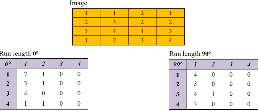
Figure 9: An example showing a 4×4 image having four gray levels (1-4) and the resulting gray level run length matrices for two directions... 22
Figure 11: Image (a) shows the user's selection, (b) shows the extracted line segments and the end-points after the thinning step, (c) lines segments are overlaid on the original
structure for user's revision, (e) the labeled line segments, (f) the estimation of the Arc
length, (g) the estimation of the chord length, and (h) the final tortuosity results... 28
Figure 12: Image (a) shows the user's input as a blue line, and (b) shows the output table contains the length and the angle results... 29
Figure 13: Image (a) shows the isosurface rendering by MATLAB functions (~ 1h.), (b) shows MATVK volume rendering through MATLAB (~ 10sec.)... 30
Figure 14: The figure shows different projections of cell formation due to the pressure exposure. (a) shows low-pressure exposure with shorter branches. (b) shows
high-pressure exposure which forms thick bands in the center of the gel, while (c) shows the
sham formation with less structure at the bottom of the gel... 33
Figure 15: The figure shows the developed GUI used to produce the results. The GUI
includes all the needed operations to analyze the vascular network using the proposed
work... 34
Figure 16: The figure shows different intensity arrangements and their corresponding
GLCM textural values... 60
Figure. 17. The figure shows different intensity arrangements and their corresponding
List of Tables
Table 1: Different orientation angles in three planes... 30
Table 2: Results obtained during the (GLCM) textural analysis, where tables 2.1 - 2.5 are the results for different frequency and pressure settings. Please see section 3.3 for
abbreviations...45
Table 3: Results obtained during the (GLRLM) textural analysis, where tables 3.1 – 3.5 are the results for different frequency and pressure settings. Please see section 3.3 for
abbreviations... 46
Table 4: Results obtained during the volumetric analysis, where tables 4.1 - 4.5 are the results for different frequency and pressure settings... 47
Table 5: Table 5. Results obtained during the GLCM textural analysis, where tables 5.1 - 5.6 are the results for experiment 1,2, and 3, while tables 5.7 - 5.10 are for experiment 4
and 5. Table 5.11 is for averaged sham... 54
Table 6:Table 5. Results obtained during the GLCM textural analysis, where tables 5.1 - 5.6 are the results for experiment 1,2, and 3, while tables 5.7 - 5.10 are for experiment 4
and 5. Table 5.11 is for averaged sham... 56
Table 7:Table 5. Results obtained during the GLCM textural analysis, where tables 5.1 - 5.6 are the results for experiment 1,2, and 3, while tables 5.7 - 5.10 are for experiment 4
Chapter 1
INTRODUCTION
1.1 OBJECTIVES AND MOTIVATIONS
Microbiological three-dimensional image analysis is rapidly becoming more
interesting to researchers, due to the huge image data produced by modern scanning tools
such as Mirco-CT, Confocal microscope, and Multi-photon microscope. This type of
analysis provides microbiological scientists with a solid ground to support their
qualitative observations using parametric quantification. The need for quantification
algorithms that efficiently provide a comprehensive three-dimensional analysis, by
quantifying the biological heterogeneity and the morphological characteristics while
providing a three-dimensional volume reconstruction all in one package, laid the
foundation of this work to provide a simple and easy-to-use Graphical User Interface
(GUI) that assists the scientists working in the field of artificial tissue engineering in
quantifying their observations.
1.2 LITERATURE REVIEW
Qualitative image analysis usually tries to differentiate between sets of
experiments by examining the image data manually and using a single image at a time
without quantitative parameters to support their observations. Many methodologies have
been proposed in the past to provide a solution to this problem. Some algorithms tackled
a single quantification problem such as counting cells or tortuosity. Other algorithms
provided either a full textural or volumetric quantification alongside with a reconstruction
The authors in [1] developed a two-dimensional automatic counting of cell colonies
algorithm that was divided into two stages. The first stage was developed to target cell
types that have a good contrast with respect to the background. Methods such as
background subtraction, edge detection, and morphological operations were used in this
stage. The second stage targeted the ill-defined or fuzzy colonies with low contrast by
using the edge information with a compact Hough transform to enhance circular shapes
while suppressing straight lines. However, the algorithm didn't provide any quantification
features beyond the counting algorithm. In [2], the authors developed a two stage
automatic segmentation algorithm to extract and quantify three-dimensional mouse
embryonic cell images produced by a fluorescence microscope. Prior to segmentation, a
two-dimensional preprocessing operations using top-hat transform, automatic
thresholding, masking, and median filtering were applied to eliminate the effect of bright
condensed regions. The first step in the segmentation process involved a
dimensional adaptive thresholding mechanism to extract complete cell clusters. A
three-dimensional Euclidean distance and watershed segmentation were then applied to
subdivide cellular regions. In the second step, the algorithm utilized a three-dimensional
level set algorithm operating on the Laplacian images to determine fuzzy borders that
weren't detected by thresholding. The quantification measurements were performed
semi-automatically, however, the reported features only included nuclei volume and distances
to the nuclear centers and peripheries.
In [3], Textural features were included alongside with a single morphological
measurement. The study used co-occurrence matrix calculation [4] to identify between
utilized to classify normal tissues. Even though this study doesn't provide the biological
meaning of the textural features, it shows that textural techniques are useful to
discriminate between pathological status of tissues. On the other hand, the algorithm
didn't provide any structural information.
For a full volumetric quantification [5,6], a three-dimensional algorithm to
quantify microvascular network of human cerebral cortex was introduced in [5]. The
images were captured using confocal microscope, and a preprocessing stage using
two-dimensional median filtering was applied. The algorithm provided comprehensive
three-dimensional quantification parameters such as microvessel density, orientations,
distances, number of segments, lengths, volume. However in [6], the algorithm included
tortuosity as a measurement for complex vascular networks, neither algorithm provided
any textural quantification. The work in [7,9] provided a full and complete quantification
by utilizing both textural and volumetric measurements. In [7], the developed algorithm
implemented a two-dimensional quantification of biofilm images. It utilized three
parameters evaluated using Gray Level Concurrence Matrix (GLCM) to quantify textural
information, while two-dimensional areal features such as porosity, fractal dimension,
and run length were used to quantify structural information. The authors in [8] decided to
take the quantification to a further step. Their developed algorithm didn't include textural
analysis, but it expanded the structural parameters to three-dimensional volumetric
parameters while adding more measurements. As a full improvement over [7,8], the
algorithm developed in [9] included a three-dimensional textural analysis alongside a
three-dimensional volumetric analysis. The developed software expanded the GLCM to a
Besides evaluating four volumetric features, the authors in [10] introduced a
three-dimensional reconstruction algorithm for cell nuclei. Their algorithm proposed
surface rendering and volume rendering methods written in C++ language and OpenGL.
In volume rendering, the algorithm separated volumetric data set into structural units by
three-dimensional labeling. After adding coordinates, intensities, and gradient vectors
information to the structural units, a bilinear interpolation scheme was utilized to
generate new values between the actual voxels. By using ray casting graphical algorithm
and assigning different colors and opacities to the voxels, the algorithm enabled
three-dimensional view from two-three-dimensional stacks of images, while no textural
quantification were reported in this study. Other techniques include registration before
the reconstruction as in [11]. The reported images show that the algorithm displayed a
solid three-dimensional object that enabled viewing front faces of the rendered volume
only. However, to view dept, the authors provided a displaying method that utilizes x, y,
z plane images to intersect at the desired point of interest.
Other techniques utilize the information such as diameter, angle, and length
extracted from volumetric analysis to reconstruct three-dimensional objects by assuming
cylindrical shapes that vary according to the previously mention features [12]. The
reconstruction method wasn't reported in the previous reference. For more information
about other techniques, the reader is referred to [13,14,15], where in [15] a recent full
1.3 CONTRIBUTION
Due to the novelty of the microbiological engineering technique used to induce
different vasculature networks, to the best of our knowledge, we believe there is no
preliminary work on quantitative image analysis and three-dimensional visualization of
Ultrasound Standing Wave Field (USWF) induced vasculature networks. In this work, we
present an algorithm that quantifies three-dimensional vasculature networks in
engineered tissues. Our algorithm includes two different three-dimensional textural
analyses evaluated from nine directions as an improvement on the algorithm presented in
[9] to quantify the heterogeneity of our induced patterns. The algorithm starts with an
enhancement process followed by a simple segmentation using threshold technique to
eliminate background noise and uneven illumination. A three-dimensional connected
component analysis is applied in the following step to extract our volume of interest. As a
quantification step, our textural analysis utilized four statistical features computed using
(GLCM ) method which incorporates voxels intensives to describe texture, as well as
Gray Level Run Length Matrix (GLRLM ) which adds structural information by using
run length technique. Combining both methods makes the textural quantification more
informative, where each technique explains the behavior of the features from the other
one. Also, we provide selected volumetric parameters computed in nine directions.
Finally, we introduce a very fast volume reconstruction through MATLAB environment
with the instructions on how to setup and establish this feature for future use to provide a
complete tool that helps the scientists in quantifying their observations and enables them
1.4 THESIS OUTLINE
This work is organized as follows. In Chapter 2 a background about tissue
engineering and the techniques used to create each tissue as well as the experimental data
are presented in this chapter. The proposed algorithm including the preprocessing steps
and the volume quantification in terms of textural, volumetric, tortuosity, length, and
angle measurements is presented in Chapter 3. Chapter 3 also shows the
three-dimensional volume rendering using the new rendering technique through linking
MATLAB environment with the visualization tool VTK, and describes the developed
GUI and its functions. In Chapter 4, the results are discussed by comparing the
quantitative analysis between the experimental data evaluated using the developed tool,
and show that our analysis supports the qualitative analysis. Finally, Chapter 5 draws
Chapter 2
BACKGROUND
Tissue engineering is the study of recreating or replacing diseased or damaged
organs and tissue by growing connective tissue using cells extracted from the body. This
technique allows newly developed tissues to be implanted and grown inside the donor's
body without immunological rejection. In a simple description of fabricating tissues and
organs, the cells are seeded within an appropriate microenvironment that promotes cell
communication and growth. When the cells find the growth factors, they start to multiply
in number and grow into a three-dimensional tissue. Once the tissue is ready, it is
implanted in the body and eventually the cells start their intended function. To keep the
implanted tissue functioning, blood vessels start to connect to the new tissue for
nourishment. For such a process to achieve its success, an appropriate microenvironment
that promotes tissue regeneration, as well as a rapid development of vascular networks is
needed.
To prepare the appropriate microenvironment, two different techniques were
reported to organize cells in complex patterns. In the first approach, pre-designed
micro-patterns are used to direct the cells to create complex structures, while in the second
approach an external force is applied to direct the cells to a certain location. Different
forces such as fluidic, magnetic, electro kinetic or optical are reported in the literature.
On the other hand, to vascularize engineered tissue, two general strategies are under
development. The first strategy depends on the natural growth of the body's blood vessels
to attach with the implanted tissue in order to form a vascular network inside it. Such a
process is reported to be slow, which can compromise tissue viability. As an
the vascular network within the engineered tissue prior to the implantation to minimize
the perfusion time after the implantation.
In this work, we utilize image processing techniques to quantitatively characterize
vascular networks induced by the recent novel application, which utilized (USWF) to
vascularize engineered tissues, as reported in [16,17,18].
2.1 EXPERIMENTAL DATA
Ultrasound Standing Wave Fields (USWF) has been demonstrated to
non-invasively control the spatial distributions of cells within three-dimensional,
collagen-based engineered tissues. Ultrasound-induced alignment of mouse embryonic
myofibroblasts in collagen gels increases cell contractility and cell-mediated extracellular
matrix reorganization. Noninvasive organization of endothelial cells within collagen gels
accelerates the formation of capillary sprouts that mature into branching networks
throughout the three-dimensional hydrogel. Both the rate of formation and morphology of
the resultant vascular network are dependent upon the ultrasound field parameters used to
produce the cellular alignment. Multi-photon microscopy imaging techniques are
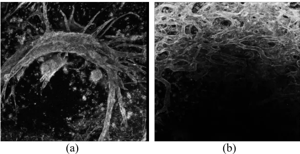
employed to visualize these branching networks, as shown in Figure 1.
Figure 1. (a) 2 MHz - 0.2 MPa image, (b) 1 MHz - 0.1 MPa image
[image:19.612.146.453.531.689.2]It was observed that at 1MHz, changing the pressure amplitude from low to high
resulted in loosely aggregated cell bands at low pressure, while dense cell bands were
formed at high pressure. Based on these differences in initial cell band density, we
observed that the resulting vascular structure differed. Loosely aggregated cell bands led
to the formation of dense vascular network. On the other hand, densely packed cell bands
formed into sprouting networks with a vascular tree-like morphology. In 2MHz, the
(USWF) pattern differs and the cell bands that are formed are closer together than those
formed at 1 MHz. However, the low and high pressure amplitudes chosen for the 2 MHz
exposures resulted in similar initial cell band density than the 1 MHz pressures used. So
the low pressure of 0.08 MPa results in loosely aggregated cell bands while the high
pressure of 0.2 MPa results in densely packed cell bands. Human Umbilical Vein
Endothelial Cells (HUVEC) were suspended in an unpolymerized type I collagen
solution and were exposed to either a 1 or 2 MHz (USWF) at various (USWF) peak
positive pressure amplitudes (1 MHz - sham, 0.1 MPa, 0.3 MPa; 2 MHz - sham, 0.08
MPa, 0.2 MPa). Collagen solutions were allowed to polymerize during the 15 min
exposure period to effectively maintain (USWF) induced cell alignment after removal of
the sound field. Exposure of (HUVEC) at the stated pressures resulted in either a
homogeneous cell distribution (sham exposure), loosely aggregated cell bands (0.1 MPa
at 1 MHz and 0.08 MPa at 2 MHz), or densely packed cell bands (0.3 MPa at 1 MHz and
0.2 MPa at 2 MHz). Samples were incubated for 10 days post (USWF) exposure and then
fixed in 4% paraformaldehyde. These experiments were repeated three times for each
condition. Standard immunofluorescence protocols were used to label (HUVEC)
staining with (DAPI). Samples were then examined using multi-photon
immunofluorescence microscopy to noninvasively scan through the three-dimensional
volume of the engineered tissue. Images were collected in the z-direction in 1 μm step
size generating stacks of 300 to 400 images. The spatial dimensions of each voxel are 2.5
x 2.5 x 1 μm3
.
In this study, we utilize stacks of multi-photon microscopy images to develop
three-dimensional textural and volumetric image analysis techniques to quantitatively
Chapter 3
PROPOSED ALGORITHM
To better understand, compare, and monitor the samples development, a
three-dimensional image analysis to quantify the volume structure is needed. A preprocessing
stage is required to enhance the stack of images before any further calculation. Figure 2
describes the entire process in terms of a flowchart.
[image:22.612.112.520.229.672.2]3D-Median 3D-Smoothing Thresholding 3D-Connected Component Analysis Volume Stack Intensity Rescaling CLAHE Textural Analysis 3D-GLRLM 3D-GLCM Volumetric Analysis 3D-Reconstruction Volume Visualization P re pro ce ss ing Vo lum e Seg menta tio n
3.1 Preprocessing
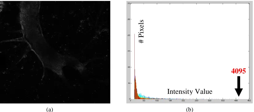
Multi-photon microscopy produces 16-bit depth images, however after close
examination, three issues were identified. First, even though the images are stored in
16-bit depth, their gray level values never exceed the value of 4096, which means that the
images, in fact, are 12-bit depth as shown in Figure 3 (b). To process and display the
images without changing their intensity distribution, they were normalized by dividing
each one by the maximum value.
Second, the intensity distribution of the images follows a very narrow unimodal
histogram centered at low intensity values as shown in Figure 3 (b). Such distribution
produces poor, low-contrast images, which are difficult to deal with. To overcome this
issue, a Contrast Limited Adaptive Histogram Equalization (CLAHE) was applied with a
7 x 7 pixels window size in order to enhance the contrast for better processing, while
preventing the over amplification of noise that global or adaptive histogram equalization
can produce in such cases. Histogram Equalization (HE) tries to transform the pixel
4095
Figure 3. (a) A single image of one sample , and (b) the corresponding histogram of the image in (a). The histogram shows a narrow distribution as well as the maximum gray level value which doesn't exceed 4095.
(a) (b)
Intensity Value
# P
[image:23.612.105.518.273.455.2]values of an image so that they occupy the full range of intensities regardless of the
histogram distribution [19-20]. Assume Pr(rk)is the normalized histogram of a given
image, where k=0,2,...,L-1 is the intensity level, and L is the number of gray levels. The
goal of the process is to generate an image with equally likely intensity values. The
normalized histogram serves as a Probability Density Function (PDF), where each single
value refers to the probability of occurrence of each gray level in the image. To transform
the random (PDF) of the image into a uniform distribution, an equalization
transformation function is used as in Eq. (1)
k j j k j j r k k MN n L r P L r T S 0 0 ) 1 ( ) ( ) 1 ( )( (1)
where Skis the new distribution and T(rk) is the transformation function modeled as the
Cumulative Distribution Function (CDF) of the original histogram. The constant MN is
the number of pixels in the image, while njrefers to the number of pixels in gray level j.
Since (HE) applies the transformation over the entire histogram as a whole, a huge noise
amplification is a natural result especially for narrow histogram distributions. Adaptive
Histogram Equalization (AHE) has the advantage of being applied locally by dividing the
image into small regions and performing (HE) on each single region separately or
overlapping[19,20]. The results of the (AHE) hold great improvement in our images, but
noise amplification still exist which produces unwanted regions at the segmentation step.
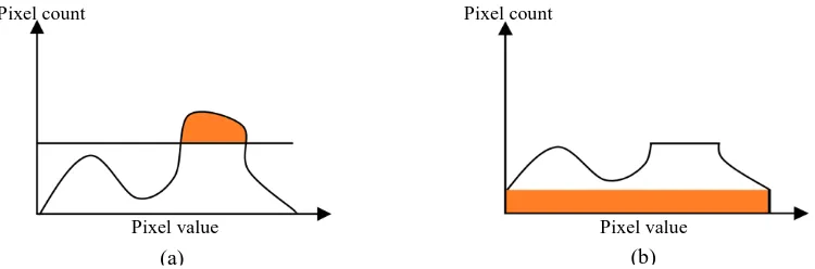
In (CLAHE), the height of the histogram is clipped at a certain level, enforcing a
maximum on the counts of the histogram that in return will limit the contrast
enhancement and the noise amplification [21]. Then the clipped regions of the histogram
mapped to the full output intensity range as described in Figure 4. Different results are
shown in Figure 5 after further enhancement for displaying purpose.
Pixel value Pixel value
Pixel count Pixel count
Figure 4. (a) The original histogram with the clipped region before redistribution, and (b) the clipped region is distributed uniformly throughout the histogram.
(a) (b)
Figure 5. (a) The original image, (b) global histogram equalization, (c) adaptive histogram equalization, and (d) with Contrast Limited Adaptive Histogram Equalization. The red circles shows the level of noise in the same region, while the yellow circles shows the effect of preserving structural regions.
(a) (b)
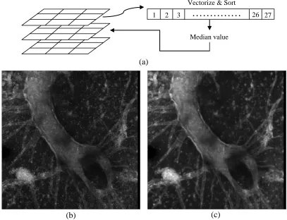
[image:25.612.112.487.134.258.2] [image:25.612.123.485.310.640.2]The third issue was due to the staining of the samples, where cellular debris is
captured alongside the vasculature structure which affects the images with a salt and
pepper-type noise. To remove such noise, we utilized a three-dimensional median
filtering algorithm with a cube of 3 x 3 x 3 voxels as shown in Figure 6.
Combining those preprocessing steps results in noise reduction while maintaining
the high spatial frequency content in each image. It is important that the three steps
mentioned above follow a certain order. At first we rescaled the intensities, then we
applied median filtering, and at the end we performed the intensity enhancement using
(CLAHE). Putting the median filtering before the (CLAHE) prevented the salt and
pepper noise enhancement alongside the actual biological structure.
1 2 3 . . . . 26 27 Vectorize & Sort
Median value
(a)
(b) (c)
[image:26.612.102.509.187.499.2]3.2 Volume Segmentation
To achieve accurate analysis, the effect of the uneven illumination needs to be
eliminated from the background, which is produced due to the scanning process of the
samples. On the other hand, all the relatively small objects that weren't removed by the
three-dimensional median filter and don't contribute to the volume of interest need to be
removed. In order to achieve this goal, two steps were applied. The first step aims to
remove the background from each image, which will prevent the textural analysis from
producing misleading results due to uneven illumination. This is done by thresholding
each single image of the stack automatically using the mean value of each image. Other
methods such as Otsu didn't work well due to the single peaked narrow intensity
distribution of the images as shown in Figure 7.
However, an effect of over quantification might result due to small gaps or discontinuities
that occur after thresholding. In order to reduce this effect, a three-dimensional
smoothing filter is utilized before the thresholding step to connect such gaps between
clusters. For more information about thresholding in tissue analysis, the reader is referred
to [22], where different thresholding techniques for engineered tissue images have been
(a) (b) (c)
[image:27.612.96.521.385.536.2]evaluated and discussed. The second step includes a three-dimensional connected
component analysis, where a 26-connectivity was used to ensure all the neighbors of each
voxel are covered. Any set of pixels which is not separated by a boundary is considered a
connected component. In order to extract the connected regions in an image, a labeling
step is required. Different segmentation algorithms ranging from simple thresholding to
more advanced techniques such as region growing and K-means clustering are used
before the labeling step. It is worth mentioning that advanced segmentation algorithms
incorporate labeling within the segmentation algorithm when providing the final results.
To label binary images, different gray level values starting from 1 to the number of the
connected regions are assigned to each region. Different searching neighborhoods
(4,8-connected neighborhood for two-dimensional images, and 6,18,26-(4,8-connected
neighborhood for three-dimensional volumes) are used for different connectivity options.
Filtering the connected components by size enables further processing over the extracted
regions. By choosing different connected volume sizes and visually inspecting the results,
we found that the volume of interest always gets extracted by choosing the largest
connected volume. This step will ensure a connectivity of the volume of interest, while
removing other regions that may contribute as noise as shown in Figure 8.
3.3 Textural Quantification
We recognize texture when we look at different patterns, but it is difficult to
define it. For our application we define texture analysis as the ability to differentiate
between different pattern arrangements due to the existence of repetitive, random, or
classification, where producing a classification map of the identified textural regions are
required, and textural segmentation which divides the image into none overlapping
regions according to their textural properties. Our textural analysis aims mainly to
describe the textural changes that occur in different induced vascular networks when
being exposed to different (USWF) settings more than a classification or a segmentation
process. Textural features can be calculated by statistical methods, geometric methods,
model based methods, or signal processing methods such as (GLCM), Voronoi
Tessellation, Fractals, and Fourier transform respectively [23]. Since our work utilizes
statistical methods, we should explain two types of statistical concepts:
i) First-order statistics: which measures a probability of observing gray levels at a
randomly selected location in an image. This type of statistics doesn't incorporate pixel
position or the effect of the neighboring pixels, but only depends on individual pixel
value. Such statistics can be calculated from the histogram such as the average image
intensity.
ii) Second-order statistics: which takes into account the likelihood of observing
the gray level values in the neighborhood at different distances and orientations. In our
(a) (b) (c)
[image:29.612.93.518.73.213.2]work we included two different textural analyses belonging to this group, since they
incorporate pixel location, orientation, and neighboring pixels information.
3.3.1 Gray Level Co-occurrence Matrix (GLCM)
The Haralick (GLCM) [24] is one of the most popular methods that utilize pixel variation
statistics in textural analysis. it uses a dependence matrix that represents the distribution
of change in gray level values of neighboring pixels. To evaluate the dependence matrix,
three different parameters should be pre-set in order to achieve the desired accuracy in
determining the textural features as follow.
i) Quantization Levels: the size of the (GLCM) is dependent on the quantization
level, since it is a square matrix with a dimension estimated by the maximum gray value
in an image. When more levels are included in the calculation, an increase of the
accuracy is achieved, however, the computational cost is increased as well and vice versa.
ii) Displacement: this parameter defines the neighboring pixels to be compared
with the current pixel. Applying a large displacement value results is a (GLCM) that
doesn't capture detailed texture, while the opposite is true as well.
iii) Orientation: it defines the direction in which the texture is being estimated.
Since each pixel has eight neighboring pixels, eight orientation angles which are 0°, 45°,
90°, 135°, 180°, 225°, 270°, and 315° are defined. However, evaluating the texture in 0°
or 180° will produce the same value for a textural feature. Since this is true for the rest of
recommended that one should estimate the textural features in all four directions in order
to avoid rotational errors and to capture every possible textural information as well.
In our work, the previous parameters were chosen as follow: different
quantization levels varying from 8 to 256 were tested for textural quantification, however
huge differences in values were observed; therefore we used the quantization level of 256
for this analysis by utilizing uniform quantization. Levels higher than 256 were not used
due to processing time. A displacement of value 1 was also chosen in order to capture the
micro-scale textural changes that occur in the vascular network. Finally, since our
samples are three-dimensional objects, we extended the orientations to cover nine
directions in three planes as shown in Table 1.
Plane XY YZ XZ
Angle 0° 45° 90° 135° 45° 90° 135° 45° 135°
In [24], eight textural features can be evaluated from (GLCM), but in this
application we chose four of them which can be interpreted into a physical meaning
describing the textural changes in our samples. The four textural parameters were
calculated over the largest connected volume as follow:
i) Entropy (ENT)
Entropy is a measurement of randomness and is defined by
1 0 1 0 )) , ( log( ) , ( N i N j j i p j i pENT (2)
where N is the number of gray levels in the image after quantization, p(i,j) is the
(GLCM) will contain many elements of small values, which results in a very large
entropy value. In other words, a random texture will result in higher entropy values,
while a smoother texture will result in lower entropy values. In our case, the entropy can
serve also as a complexity measurement, where a higher value refers to a more complex
structure.
ii) Energy (ENE)
Energy is also called Angular Second Moment (ASM). This parameter was
utilized as a measurement of cluster repetition and uniformity, and it is defined by
1 0 1 0 2 ) , ( N i N j j i pENE (3)
For this parameter to reach its maximum value of 1, a few elements in the GLCM should
be close to 1, while many elements should be close to 0. In other words, a higher energy
value means more periodic and uniform clusters in the volume, while the ideal case
happens when the volume has a constant intensity level where the energy value equals 1.
iii) Contrast (CON)
Contrast measures the difference between the highest and the lowest intensity
values of contiguous pixels and it is defined by
1 0 1 0 2 ) ( ) , ( N i N j j i j i pCON (4)
where the values range between 0 and (N-1)2. Higher contrast corresponds to busier
texture and sharper, more frequent transitions between the gray levels.
iv) Homogeneity (HOM)
Homogeneity measures the similarity and the smoothness between the intensity
values of neighboring pixels. It is defined by
(
( 4)
1 0 1 0 2 ) ( 1 ) , ( N i Nj i j
j i p
HOM (5)
where higher homogeneity corresponds to smoother and more similar regions in the
volume.
3.3.2 Gray Level Run Length Matrix (GLRLM)
Run length analysis captures the textural information in a specific direction. A run is
defined as a group of consecutive pixels that have the same gray level value along a
specific orientation. Fine texture tends to contain a higher number of short runs with
similar intensities, while coarse texture has longer runs [25].
The run length matrix R is defined as follows: the elements R(i,j) refer to the number of
runs with pixels of gray levels (i) and length of runs equal (j) along a certain orientation.
The size of the matrix is M by N, where M is the number of the gray levels in the image,
while N is the maximum possible run across the image. The following figure shows a
[image:33.612.93.529.497.685.2]simple example describing the calculation of a run length matrix.
(
5)
Different numerical measurements of texture can be estimated from this matrix. The
advantage of this analysis is that it provides textural information while incorporating
structural information while the calculation is done. As a result of this an explanation of
the GLCM features' behavior is found here. For example, an image that has a high
number of long runs results in a low entropy value and a high homogeneity value, while
the opposite is also true. In [26], the authors suggested that the gray-level values to be
grouped into 8 sets (levels) for a 64-levels image, and the run lengths into 6 sets for a 64
by 64 image. We believe the reason behind this is to avoid irrelevant counting of very
small runs and very close values of intensity levels, which may contribute in a negative
way to the analysis. Since our analysis is applied over the largest connected volume with
no background intensity variation or noise, we need every single run length of the volume
to be counted. Also, due to having 256 intensity levels, we grouped the gray-level values
into 16 different sets. The following five features are described for further explanation.
i) Short Run Emphasis (SRE)
This feature measures and emphasizes the short runs in the image, and it is
calculated by
N i M j N i i M j j i R j j i R SRE 1 1 1 2 ) , ( ) , ( (6)where N and M are the row number and the column number of the GLRLM respectively,
while R(i,j) is the entry value at location (i,j). A higher value corresponds to a higher
amount of short runs in the image, which indicates that the image contains a
ii) Long Run Emphasis (LRE)
This feature emphasizes the long runs in the image, and it is calculated by
N i M j N i i M j j i R j i R j LRE 1 1 1 2 ) , ( ) , ( (8)where higher values correspond to a higher amount of long runs in the image, which
indicates that the image contains bigger regions of similar structural texture.
iii) Gray Level Non-uniformity (GLN)
The output of this function measures the intensity variation throughout an image,
and it is calculated by
N i M j N i i M j j i R j i R GLN 1 1 2 1 ) , ( ) , ( (9)The lowest value occurs when the runs of the intensity levels are equally distributed
throughout the image, higher values correspond to a fine textural structure.
iv) Run Length Non-uniformity (RLN)
This feature measures the distribution of the runs throughout the lengths in the
image, and it is defined by
N i M j M i j N i j i R j i R RLN 1 1 2 1 ) , ( ) , ( (10)The function has a low value when the image has a single intensity value, since the
v) Run Percentage (RP)
The output of this function is a ratio of the total number of the runs to the total
number of pixels K in the image and it is calculated by
K j i R RP
N
i i
M
j
1
) , (
(11)
where K is also known as the total possible runs if all the intensities have a run length of
one. By combining the two previously mentioned methods, nine different parameters
evaluated in nine directions provide us with a complete picture of how the characteristics
of samples exposed to different regimes differ from each other. For better understanding
of textural parameters, we included synthetic images that explain the differences between
3.4 Volumetric Quantification
Volumetric parameters were evaluated on the three-dimensional binary version of
the images to quantify the morphological information of the induced vasculature
networks. Features such as growth direction and volume percentage are presented in this
section. We also utilized the two-dimensional z-projection images to estimate the
tortuosity and to provide length and angle measurements as additional, but important
features.
3.4.1. Growth Direction
This parameter is computed in order to find in which direction the branching
network is growing. To evaluate this parameter, an average run length algorithm was also
utilized in the nine directions described in Table 1. Higher values result when longer
connected regions are examined. For example, if we measure the growth in XY-plane
with 0º between two different objects, the object with the higher value will have a larger
connected object in that direction.
3.4.2 Volume Percentage (VP)
This feature measures how much the extracted volume covers from the total size
of the sample, and it is calculated by dividing the number of voxels of the extracted
volume of interest over the total number of voxels of the sample. This analysis gives us
an indication of how changes in frequency and pressure regimes will affect the size of the
formed network structures. The actual size of each volume can be found by multiplying
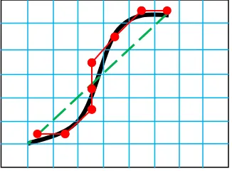
3.4.3 Tortuosity
This feature is generally used in estimating the retinal blood vessels curvature, which
provides an indication about retinal diseases since normal vessels tend to be straight and
gently curved [27]. Different methods were reported in the literature to estimate this
feature [27,28,29]. The method named Arc-Chord Ratio (ACR) is used in this work,
which is calculated as follows: assume a line segment S, as shown in Figure 10, has an
Arc length L and a chord length C, then the tortuosity
(S) is computed as
C L S) (
(12)
where L is computed as the sum of the Euclidean distances between the connected pixels
of the line segment, while C is calculated as the Euclidean distance between the end
points of the same segment. This ratio equals 1 for straight line and ∞ for a circle.
In our work, in order to estimate the tortuosity, many steps are taken to find both
distances to calculate this feature. The user has to select the region for which he/she
wants to estimate this feature manually, and then a thinning algorithm that simplifies the
structure into lines is applied. The lines are then separated into different segments
(branches) in order to find the end-points. By labeling the different line segments and
[image:38.612.225.388.402.522.2]extracting the end points, the distance estimation then becomes an easy step and the
tortuosity is calculated. The following Figure shows the tortuosity estimation process.
(a) (b) (c)
(e) (f) (g)
z-projected image...PLEASE SELECT AN R-I-O SEGMENTS AND END POINTS OVERLAYED IMAGE
SEGMENTS LABELS SEGMENTS PATH LENGTH
* 204.978 pixels * 78.841 pixels * 29.971 pixels
* 98.510 pixels
* 225.640 pixels * 188.380 pixels
* 82.385 pixels
* 275.475 pixels
* 146.610 pixels
SEGMENTS END POINTS DISTANCES
* 191.107 pixels * 72.918 pixels * 27.731 pixels
* 96.333 pixels
* 206.155 pixels * 174.943 pixels
* 77.058 pixels
* 257.070 pixels
* 131.674 pixels
SEGMENTS END POINTS DISTANCES
* 1.073 pixels * 1.081 pixels * 1.081 pixels
* 1.023 pixels
* 1.095 pixels * 1.077 pixels
* 1.069 pixels
* 1.072 pixels
* 1.113 pixels
(h)
[image:39.612.98.517.119.666.2]3.4.3 Length and Angle Estimation
These measurements are also estimated by utilizing the z-projection images. The
user will draw a line over the structure that he/she wants to find the value for, then the
algorithm will find the distance between the end-points of the line as the length in pixels,
while the angle is estimated by finding the angle between the drawn line and the positive
x-axis. Figure 12 shows an example of the user selection and the estimated
measurements.
z-projected image...PLEASE SELECT AN R-I-O
[image:40.612.150.479.269.663.2]259.88
Figure 12. Image (a) shows the user's input as a blue line, and (b) shows the output table contains the length and the angle results.
(a)
3.5 Volume Visualization
In order for scientists working in microscopy to get the full benefits of our tool, a
three-dimensional visualization is needed. Using the MATLAB function to produce a
volume of approximately 400 images, it took the algorithm close to 1 hour to produce an
iso-surface rendering, which lacks the appropriate light effect and speed needed to zoom
and rotate the volume. In order to boost the three-dimensional reconstruction through
MATLAB, a group of researchers developed a three-dimensional reconstruction
extension for MATLAB, using the visualization capabilities of VTK called MATVTK
[30]. To the best of our knowledge, a step by step manual that helps setting up this tool is
not widely available. After collecting information from different places and
troubleshooting, we managed to get the tool to work and to be fully integrated with
MATLAB. Due to this reason, we are providing a full setup instructions (see Appendix
(C) on how to compile VTK and MATVTK from source code and how to integrate it
with MATLAB for any further use in any research requires a three-dimensional
visualization. Figure 13 shows the isosurface rendering by MATLAB versus the volume
rendering by MATLAB using MATVTK.
Figure 13. Image (a) shows the isosurface rendering by MATLAB functions (~ 1h.), (b) shows MATVK volume rendering through MATLAB (~ 10sec.).
[image:41.612.117.518.526.670.2]Chapter 4
RESULTS
In this paper, we compare different experimental conditions consisting of two
different frequency settings and pressure regimes. We use the sham samples as a
reference to compare to. Also, since the experiments are independent, the sham results
from all experiments were averaged. This step was taken after analyzing each sham
sample and not finding noticeable differences among them. Tables 2 and 3 list textural
parameters calculated by the (GLCM) and (GLRLM) methods respectively, while Table
4 shows the results calculated for the volumetric analysis.
In Table 2, entropy is highest for the low peak positive pressure cases in both
frequency regimes, i.e., 0.1 MPa for 1 MHz, and 0.08 MPa for 2 MHz. These entropy
values indicate the disruption of the network appearance compared to the sham values,
which show more complex structure. On the other hand, the entropy value for the high
peak positive pressure cases in both frequency settings is lowest, since the images contain
highly packed sprouts with lower structural complexity. These results are further
supported be the fact that energy and homogeneity are lowest, while contrast is maximum
in the low-pressure cases, while the opposite is true for the high-pressure cases. By taking
a closer look at experiment 2 and 3 (Appendix A), we find that entropy is a bit higher
than the averaged sham, while the energy is lower. However, homogeneity and contrast
follows the previous observations, while no changes occurred in the low pressure
samples. The reason for this is the fact that there is more cell communication in the high
pressure samples compared to the sham samples, due to the absence of the pressure effect
in the later one. At this stage, we see how the (GLRLM) analysis helps in understanding
pressure samples have lower number of short runs, run length non-uniformity, and run
percentage, which supports our reasoning above.
In Table 3, the high-pressure samples have lower values of short runs and higher
long run values compared to the sham samples. On the other hand, the opposite is true for
the low-pressure samples. This indicates that the high-pressure regime tends to form
denser, more uniform, and smoother regions with bands and long sprouts. However, the
low pressure setting wasn't enough to force the cells to form thick bands, but it was
enough to form short branches when comparing to the sham samples. This conclusion is
further supported by the difference of the values in the rest of the features. Other
parameters presented in the literature [31,32] which will increase the dimensionality and
the complexity in interpreting the results were not included.
Table 4 shows that the high-pressure cases have higher volumetric run length
values than the low-pressure cases compared to sham samples, except for the z-direction,
due to the morphological structure of the low-pressure setting as shown in Figure 14 (a).
Also, it is worth mentioning that the ratio between the z-direction run length and the other
directions shows that the high-pressure setting tends to form structures in the center of the
plate as shown in Figure 14 (b), while the low-pressure samples tends to grow vertically
compared to sham networks which lay down at the bottom of the plate as shown in Figure
14 (c).
The absence of (USWF) on the sham samples result in a lower rate of biological
communication between the cells, which is supported by the fact that they have lower
volume percentage (VP) in Table 4. On the other hand, low-pressure samples have the
enough to pack them into thick bands. The values for the high-pressure samples tend to
be in-between except for the 2MHz samples, which we noticed that they were always
lower in this case. We relate this observation to the effect of changing the frequency to a
higher setting, which induces the formation of bands more than in the 1MHz samples.
The overall results show that the high-pressure samples have smoother, more
uniform, longer, and densely packed structure, while the low-pressure samples tends to
have non-uniform, more heterogeneous, shorter, and unpacked network structure.
Therefore, the quantitative results presented in this work obtained using textural and
volumetric analysis of three-dimensional vascular structures in engineered tissues support
the qualitative observations made in [18], that different vascular network morphologies
are formed when low versus high pressure amplitudes were used to organize cells within
the tissue constructs. Figure 15 shows the GUI that was developed and used to produce
[image:44.612.93.518.435.586.2]these results.
Figure. 14. The figure shows different projections of cell formation due to the pressure exposure. (a) shows low-pressure exposure with shorter branches. (b) shows high-low-pressure exposure which forms thick bands in the center of the gel, while (c) shows the sham formation with less structure at the bottom of the gel.
Table 2. Results obtained during the GLCM textural analysis, where tables 2.1 - 2.5 are the results for different frequency and pressure settings. Please see section 3.3 for abbreviations
Table 2.1. GLCM results for 1MHz - 0.3 MPa Table 2.2. GLCM results for 1MHz - 0.1 MPa
Table 2.3. GLCM results Averaged SHAM
[image:46.612.88.527.110.596.2]Table 3. Results obtained during the GLRLM textural analysis, where tables 3.1 – 3.5 are the results for different frequency and pressure settings. Please see section 3.3 for abbreviations
Table 3.1. GLRLM results for 1MHz - 0.3 MPa Table 3.2. GLRLM results for 1MHz - 0.1 MPa
Table 3.3. GLRLM results for Averaged SHAM
[image:47.612.55.575.522.684.2]Table 4. Results obtained during the volumetric analysis, where tables 4.1 - 4.5 are the results for different frequency and pressure settings.
Table 4.1. Volumetric results for 1MHz - 0.3 MPa Table 4.2. Volumetric results for 1MHz - 0.1 MPa
Table 4.3. Volumetric results for Averaged SHAM
[image:48.612.89.519.84.709.2]Chapter 5
CONCLUSIONS AND FUTURE WORK
In this work, a tool that analyzes three-dimensional vasculature networks in engineered
tissues alongside providing a three-dimensional volume rendering was proposed. The
algorithm used textural and volumetric parameters for quantitative analysis to provide a
more objective and reliable monitoring as well as a quantitative comparison between the
structures. We showed that combining two different textural quantification methods
provide a comprehensive overview about the structure's heterogeneity. We also showed
that expanding the analysis to cover nine orientations in quantifying textural and
volumetric features, enabled us to capture full three-dimensional changes happen
throughout our samples. Other volumetric parameters such as porosity, permeability, and
diffusion distance were not included, since they don't serve the purpose of comparing
totally different structures. Parameters such as tortuosity, length, and angle that provides
more information about the induced structures using the z-projection version of the stacks
were included. The algorithm provided a fast three-dimensional volume rendering by
linking MATLAB and VTK using the newly developed tool named MATVTK. The
algorithm is provided with a standalone (GUI) written in MATLAB, which will allow
the scientists to interact with the algorithm without the need of understanding the code.
The (GUI) also provides other functions such as viewing, filtering, or projecting the
samples using different techniques. Future work includes investigating different
sophisticated segmentation techniques beside the effect of other three-dimensional
volumetric parameters such as Three-dimensional Fractal Dimension (3D-FD), which is
commonly used in medical imaging [33], and Three-dimensional structural similarity
Bibliography
[1] P.R. Barber, B. Vojnovic, J. Kelly, C.R. Mayes, P. Mayes, M. Woodcock, and M.C.
Joiner, "Automated Counting of Mammalian Cell Colonies," Physics in Medicine and
Biology, vol., 64, pp.63-76, (2001).
[2] N. Harder, M. Bodnar, R. Elis, D.L. Spector, and K. Rohr, "3D Segmentation and
Quantification of Mouse Embryonic Stem Cells in Fluorescence Microscopy Images ,"
Biomedical Imaging: From Nano to Macro, 2011 IEEE International Symposium on,
pp.216-219, (2011).
[3] J. Diamond, N.H. Anderson, P.H. Bartels, R. Montironi, and P.W. Hamilton, "The
Use of Morphological Characteristics and Texture Analysis in the Identification of Tissue
Composition in Prostatic Neoplasia," Hum. Pathol, vol., 35, pp.1121-1131, (2004).
[4] R.M. Haralick, K. Shanmuga, and I. Dinstein, "Textural Features for Image
Classification," IEEE Transactions on Systems, Man and Cybernetics SMC3,
pp.610-621, (1973).
[5] F. Cassot, F. Lauwers, C. Fouard, S. Prohaska, and V. Lauwers-Cances, "A Novel
Three-dimensional Computer-assisted Method for A Quantitative Study of Microvascular
Networks of the Human Cerebral Cortex," Microcirculation, vol., 13, pp.1–18, (2006).
[6] P.R. Barber, S.M. Ameer-Beg, B. Vojnovic, R.J. Hodgkiss, G.M. Tozer, J. Wilson,
and V.E. Prise, "3D Imaging and Quantification of Complex Vascular Networks,"
Proceedings of SPIE-OSA Biomedical Optics, SPIE, vol., 5139, (2003).
[7] X.M. Yang, H. Beyenal, G. Harkin,, and Z. Lewandowski, "Quantifying Biofilm
Structure Using Image Analysis," Journal of Microbiological Methods, Elsevier,
[8] A. Heydron, A.T. Nielsen, M. Hentzer, C. Sternberg, M. Givskov, B.K. Ersboll, and
S. Molin, "Quantification of Biofilm Structure by the Novel Computer Program
COMSTAT," Journal of Microbiology, pp.2395-2407, (2000).
[9] H. Beyenal, C. Donovan, Z. Lewandowski, and G. Harkin, "Three-dimensional
Biofilm Structure Quantification," Journal of Microbiological Methods, Elsevier,
pp.395-413, (2004).
[10] H.J. Choi, I.H. Choi, T.Y. Kim, and H.K. Choi, "A Computerized Program for
Three-dimensional Visualization and Quantitative Analysis of Cell Nuclei," Enterprise
Networking and Computing in Healthcare Industry, Proceedings. 6th International
Workshop, pp.83- 87, (2004).
[11] F. Scarpa, D. Fiorin, and A. Ruggeri, "In Vivo Three-dimensional Recon-Struction
of the Cornea From Confocal Microscopy Images," Conference Proceedings of IEEE
Engineering in Medicine and Biology Society, pp.747–750, (2007).
[12] J. Wu, B. Rajwa, D.L. Filmer, C.M. Hoffmann, B. Yuan, C. Chiang, et al.,
"Automated Quantification and Reconstruction of Collagen Matrix From 3D Confocal
Datasets," Journal of Microscopy, vol., 210, pp.158-165, (2003).
[13] E. Kaczmarek, and R. Strzelczyk, "From Two to Three-dimensional Visualization of
Structures in Light and Confocal Microscopy – Applications for Biomedical Studies,"
Multidisciplinary Microscopy Research and Education, pp.289-295, (2005).
[14] H.J. Choi, T.Y. Kim, N.H. Cho, G.B. Jeong, Y. Huh, and H.K. Choi,
"Three-dimensional Quantitative Analysis of Cell Nuclei for Grading Renal Cell Carcinoma,"
Enterprise networking and Computing in Healthcare Industry, HEALTHCOM.