Two-tier Networks: A Stienen’s Model Base Approach
.
White Rose Research Online URL for this paper:
http://eprints.whiterose.ac.uk/113323/
Version: Accepted Version
Article:
Hernandez-Aquino, R, Zaidi, SAR, Ghogho, M orcid.org/0000-0002-0055-7867 et al. (2
more authors) (2017) Stochastic Geometric Modeling & Analysis of Non-Uniform Two-tier
Networks: A Stienen’s Model Base Approach. IEEE Transactions on Wireless
Communications. ISSN 1558-2248
https://doi.org/10.1109/TWC.2017.2682844
© IEEE 2017. This is an author produced version of a paper published in IEEE
Transactions on Wireless Communications. Personal use of this material is permitted.
Permission from IEEE must be obtained for all other uses, in any current or future media,
including reprinting/republishing this material for advertising or promotional purposes,
creating new collective works, for resale or redistribution to servers or lists, or reuse of any
copyrighted component of this work in other works. Uploaded in accordance with the
publisher's self-archiving policy.
[email protected] https://eprints.whiterose.ac.uk/ Reuse
Unless indicated otherwise, fulltext items are protected by copyright with all rights reserved. The copyright exception in section 29 of the Copyright, Designs and Patents Act 1988 allows the making of a single copy solely for the purpose of non-commercial research or private study within the limits of fair dealing. The publisher or other rights-holder may allow further reproduction and re-use of this version - refer to the White Rose Research Online record for this item. Where records identify the publisher as the copyright holder, users can verify any specific terms of use on the publisher’s website.
Takedown
If you consider content in White Rose Research Online to be in breach of UK law, please notify us by
Stochastic Geometric Modeling & Analysis of
Non-Uniform Two-tier Networks: A Stienen’s
Model Based Approach
Raul Hernandez-Aquino,
Student Member, IEEE,
Syed Ali Raza Zaidi,
Student Member, IEEE,
Mounir Ghogho,
Senior Member, IEEE,
Des McLernon,
Member, IEEE,
and Ananthram Swami,
Fellow, IEEE
Abstract—While stochastic geometric models based on Poisson point processes (PPP) provide a tractable approach for the anal-ysis of uniform two-tier network deployments, the performance evaluation of a non-uniform deployment remains an open issue which we address in this paper. This is due to the fact that smaller cells can be more efficiently deployed in areas where the QoS of traditional macro base stations is poor. Therefore, in this paper we introduce Stienen’s model which allows us to analyse such non-uniform deployment. In contrast to tradi-tional PPP based analysis, performance characterization under Stienen Model are more challenging due to location and density dependencies. However, we demonstrate that the performance can be approximated in a tractable manner. The developed statistical framework is employed to characterize the gains in terms of energy efficiency (EE) for non-uniform deployments. Results show an achievable 19% to124% improvements in the
macrocell coverage as compared to a uniform deployment, while the femtocell coverage and system EE are of the same order of magnitude for both deployments. These results are complemented with the fact that OPEX and CAPEX are reduced due to a lesser number of FAPs deployed.
Index Terms—Energy efficiency, Rayleigh fading, Poisson point process.
I. INTRODUCTION
A. Motivation
T
HE the exponential increase in both the number of users of cellular systems and their bandwidth requirements, has created the need to increase the data rates that the system can handle and improve the coverage where it is needed. However, until very recently designing for energy efficiency (EE) has not received the importance that it deserves in the development of techniques and algorithms for future wireless networks deployments. According to recent studies, around 2% of the global CO2 emissions is contributed by theInfor-mation and Communication Technology (ICT) industry [1]. In particular, the share for telecommunications is around 1%, and this is directly related to the energy used in the cellular
This work was partly supported by CONACYT, Mexico; Secretaria de Educacion Publica; the Mexican government; and U.S. Army Research Lab Grant W911NF-13-1-0216.
R. Hernandez-Aquino, S.A.R. Zaidi and D. McLernon are with the School of Electronic and Electrical Engineering, University of Leeds, Leeds, United Kingdom. email:{elrha, s.a.zaidi,d.c.mclernon}@leeds.ac.uk
M. Ghogho is with the School of Electronic and Electrical Engineering, University of Leeds, Leeds, United Kingdom and also with the International University of Rabat, Morocco. email: [email protected]
A. Swami is with the U.S. Army Research Lab, Adelphi, MD, USA (e-mail: [email protected]).
system. Moreover, about 80% of this energy is consumed by the Radio Access Network (RAN) [1]. So reducing the energy consumption in cellular networks has therefore both environmental and economical implications.
A promising solution for Next Generation Networks (NGNs) to cope with the demands for better coverage and higher data rates is the deployment of heterogeneous networks (HetNets) which consists of smaller, cheaper and less energy consuming base stations (BSs) such as femtocell access points (FAPs) overlaid with the traditional macro base station (MBS) network [2]. The use of HetNets has the potential to provide both the required coverage and increase the data rates of the users. However, realising such a potential may incur a significant energy penalty if the EE is not used as a metric to design the HetNet. This can be attributed to the fact that dense network deployment with aggressive frequency reuse does not come without increased co-channel interference. Thus network resources/available degrees-of-freedom should be engineered with the aim of maximizing EE without sacrificing the desired quality of service (QoS).
In order to characterize the performance of a large scale network, Poisson Point Processes (PPPs) [3] have frequently been used to model infrastructure-less networks such as ad-hoc [4]–[6] or femto-cell networks [7]–[11]. In these networks the randomness is an intrinsic ingredient of the network topology. Thus PPPs are a natural choice to capture the spatial dynamics. Furthermore, the use of PPPs has also been extended to model macro-cells [12]–[14], since the traditional hexagonal lattice based models only provide an upper bound on the performance of actual networks at the cost of time consuming and tedious simulations and/or numerical integrations. In contrast, PPPs have proven to be just as accurate as grid models (under certain conditions) to characterize the network performance with the advantage of an analytically tractable model.
to the edge of the cells. Moreover, it is well established that traditionally the bottleneck of the cellular system resides in the edge user performance.
Characterizing the performance of non-uniform two-tier net-works deployment is a non-trivial task. This can be attributed to the fact that within stochastic geometric analysis1 the edge of a typical Voronoi cell does not have a fixed shape. The exact geometry depends on the number of neighbors which is a random variable with unknown distribution [15]–[17]. Additionally, due to the polygonal nature of the cell edge, the distances across different edges may vary. Thus, analysing cell edge type deployments becomes challenging. Consequently, there is a need for a tractable model where non-uniform deployments (which are parametrized by the cell-size and cell-edge deployment densities) can be investigated. In this paper, we introduce Stienen’s model which can address the above mentioned challenges. Stienen’s model was originally proposed for material science related application [18].
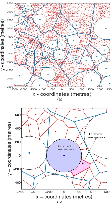
Stienen’s Model overview: Stienen’s model can be con-structed from a Poisson-Voronoi Tessellation. Assume a cel-lular network where each mobile user is associated to the closest macro BS. The complement of the coverage areas of all MBS then form a Voronoi Tessellation. For a typical MBS, a Steinen’s cell can be formed by constructing a disc whose radius is equal to half of the distance between the MBS and its nearest neighbour (see Fig. 1). Note that the Voronoi cell of the typical MBS is larger than its Stienen cell. In other words, each Voronoi cell can be decomposed into two regions, namely, the Stienen cell and its complementary area. Such decomposition of a typical Voronoi cell allows to model different deployment densities in these two areas. Moreover, as compared to traditional hardcore models such as Matern processes, the exclusion disc via Stienen’s model intrinsically captures the impact of the cell size. Since the coverage area of each MBS is not isotropic (and polygonal in nature), it would make less sense to have a fixed size disc centered at each MBS and then deploy FAPs outside such a disc. This is because some cell edges are far more closer to MBS than others. Stienen’s Model also intrinsically captures this irregularity in distances to different cell edges.
In this article, we propose an operator’s femtocell deploy-ment on areas close to the macrocell edge. As a result, we obtain an analytical framework to model non-uniform two-tier HetNet deployments via Stienen’s model. We demonstrate that19% to124% improvements are possible in the macrocell coverage as compared to the ones obtained with a uniform deployment when the same parameters are used. On the other hand, the femtocell coverage and system EE are similar in both deployments but with the main difference that the non-uniform deployment has a significant reduction of the OPEX and CAPEX due to the smaller number of smaller cells deployed.
B. Related Work
The gains in coverage, throuhgput and EE of HetNets have been analysed in several works, where the improvements have
1which is often employed to characterize the performance of large scale
cellular network
been reported for different techniques and algorithms. The EE of a two-tier network consisting of both macro- and picocells was analysed in [19] where both tiers were modelled with in-dependent PPPs. Analytical results on the coverage probability, data rates and EE (in bits/s/m−2/J) were obtained as a function of the base station densities. Also, by considering independent PPPs, [20] evaluated the EE in a scenario consisting of micro-and picocells. An optimization problem was formulated to obtain the density of picocells that maximized the EE of the network with constraints on the outage probabilities of both tiers. The study of EE with the use of PPPs was extended to the multi-antenna case in [9] and [10]. An analysis of the EE of different MIMO diversity schemes was carried out in [9] for a two-tier network consisting of macro and femtocells. The opti-mum antenna configuration and diversity schemes that yielded the maximum EE (while keeping some QoS constraints) were presented for different system parameters. Alternatively, in [10] a scenario consisting of a single macrocell overlaid with a tier of femtocells modelled with a PPP was analysed. The authors examined the throughput and the EE of a MIMO system with an opportunistic interference alignment scheme in order to mitigate interference. While the results of this works show the potential improvements in the performance of the network in terms of coverage, data rates and EE by deploying HetNets, the assumption that there is not an inter-tier dependency on the location of different inter-tiers is simply not realistic.
tier follows a Poisson hole process (PHP). Therefore, the picocells are only deployed in the locations outside a circular area surrounding a MBS with a fixed radius of exclusion. By assuming a fixed position from a typical macrocell user to its designed MBS and a typical femtocell user to its tagged pico BS, bounds on the coverage probabilities for both users are obtained.
C. Contributions
The need to plan in a more efficiently manner the deploy-ment of smaller cells, creates a challenge in the analysis of the deployment of non-uniform tiers. Therefore in this work, we propose a tractable model for the non uniform deployment of a two-tier network consisting of macro- and femtocells. While the macrocells are uniformly distributed across the service area, the FAPs are only deployed outside a given disc of radius
Rs centered at each MBS. Most of the works devoted to the
study of non-uniform BSs assume a fixed exclusion region, which lacks a sense of realistic planning from a network operator perspective, as the size of the cell determines the areas where the potential placement of smaller cells can improve the performance. Moreover, the interrelation between a cell edge user and the topology of the cell is lost. This is due to the fact that classifying a user as cell edge user depends on the location of the user in its particular serving MBS. This cannot be captured by using a fixed radius as the size and shape varies from macrocell to macrocell. In contrast with those works, we propose the use of Stienen’s model [18] to design the size of
Rs. The resulting exclusion region is a function of the size of
each Voronoi cell. The model then accounts for a more realistic model where the areas of possible femtocell locations depend on the size of the macrocell, while preserving the correlation of cell edge users with the topology of the cell. Additionally, the proposed model represents a tractable approach which can be easily scaled for a high number of femtocells deployed. The main contributions of this paper are stated as follows.
• Introducing Stiennen’s model: We propose the use of Stienen’s model [18] to characterize in a realistic manner a non-uniform deployment of femtocells overlaid to a macrocell network. In this model, a radius surrounding each MBS (Stienen radius) is designed as a function of the distance to its closest (interfering) MBS. On the other hand, the femtocell tier is deployed only in the areas outside the discs of Stienen radii. Users located in the areas enclosed by the discs of Stienen radii will be served by the macrocell tier while the users located outside these areas (edge users) will be offloaded to the femtocell tier.
• Improved edge user performance: It is universally
ac-cepted that the bottleneck of cellular networks is the edge user, which experiences the worst performance due to the high path loss perceived at a distant user and also because the distances between the serving and interfering BSs to the user have the same order of magnitude. As is shown in the results, with the proposed model, the edge user performance can be greatly increased with the deployment of femtocells, while the macrocell user performance is not significantly reduced. This in turn
helps to achieve a more balanced network throughout the entire service area.
• Characterization of coverage, throughput and EE of users
in both tiers: With the use of tools from stochastic geometry, we provide a tractable approach to characterize the performance of users in both tiers. Namely, we find expressions for the coverage probability, average user throughput and overall EE of the network.
• Improved coverage, throughput and EE: By letting users located outside the discs of Stienen’s radii to be served only by femtocells, the performance in terms of coverage, throughput and EE is improved in both tiers in compari-son with a typical deployment. On one hand, due to the fact that the users served by the macrocell tier will be closer to their serving MBS in comparison with a normal deployment, they will experience better QoS. On the other hand, given that the femtocells will only be deployed in areas where the average perceived power from a MBS is not very high, the use of resources is carried out in a more efficient manner, which is reflected in the enhanced performance.
D. Organization and notation
The rest of the paper is organized as follows. Section II introduces the system model. The coverage probability and the expected throughput in each tier for the proposed model are derived in section III. . Section IV describes the analysis of the EE for the proposed model. The numerical results are presented in Section V. Finally, conclusions are given in Section VI.
Throughout the paper the following notations are used. The notation E[X] is used to express the expected value of the random variableX. A random variableXfollowing a complex Gaussian distribution with mean µ and variance σ2 is
ex-pressed asX ∼ CN(µ, σ2). A Poisson distribution with mean µ is expressed as Pois (µ), and an exponential distribution with meanµis written asExpµ1. CDF(FX(x))and CCDF
(Fc
X(x) = 1−FX(x))stand respectively, for the cumulative
and complementary cumulative distribution function of the random variableX. We denote as FinallyB(x, D)represents the ball of radius D centered atx.
II. SYSTEM MODEL
Consider a two tier network consisting of MBSs and FAPs deployed in a given area. The MBSs are deployed across the entire area following a PPP Φm, with densityλm. The FAPs
are only deployed outside the discs of radii Rj
s centered at
each MBS located at xj ∈Φ
m, where the superscript stands
for the j-th MBS (j ∈ Φm)2. The femtocell tier is then
modelled via a PHP with effective intensity λfp, whereλf is
the original intensity of femtocells, whilepis the probability that a FAP will be located outside the discs of radii Rj
s,
∀j ∈ Φm. In this model, the users that fall within the area
2Note that we will refer toxj∈Φmandxk∈Φfto represent, respectively,
the position of the j-th andk-th points. On the other hand, we will use
j ∈ Φm and k ∈ Φf with j = 0,1, ...,|Φm|andk = 0,1, ...,|Φf|to
covered by the discs will be served by the corresponding MBS. On the other hand, the users located outside the discs will be served by the femtocell tier. The advantages of this model are two-fold: deploying only femtocells in areas where the coverage is expected to be low (near the edge of the macro cells), and improving the macrocell expected performance, since the users served by the macrocell tier will be close to their serving MBS. Users are modelled by another PPP Φu
of density λu and so, they are uniformly placed across the
service area. We assume that each user is associated with the closest MBS. This is equivalent to a user associating with the MBS which provides the highest long term expected power. In the femtocell tier, we also assume that the users are associated with the nearest FAP. Under these assumptions, the resulting association scheme is formed by two Voronoi tessellations [12], i.e. one corresponding to the macrocell tier and the other one for the femtocell tier. The Voronoi cells formed represent the coverage regions for each BS in the network.
In contrast with previous works, in this paper we propose the use of Stienen’s model to characterize the size of the macrocell coverage area, matching it with the area enclosed in the Stienen cells. Originally proposed for applications in material science, Stienen’s model [18] is described as follows. Consider the homogeneous PPP Φm modelling the positions
of the MBSs. The points generated byΦm are taken as seeds
to construct a Voronoi tesellation. Now, around each point
xj, j ∈ Φ
m (each Voronoi cell seed), a disc of radius Rjs
equal to half of the distance to the closest neighbour of xj
is placed. We can extend the model to a more general case, in which the radius Rj
s is assumed to be the product of the
closest neighbour and a scalar τ. When τ <1/2, the disc is located completely inside its Voronoi cell. On the other hand, for τ >1/2 the disc extends to other macrocells3. Note that due to the independence property of the PPP, the set of Stienen radii {Rj
s}, j ∈ Φm are all i.i.d. Therefore, we will refer to
the Stienen radius only asRsin the reminder of the paper.
To model the location dependent femtocells, the FAPs with density λf are placed uniformly only in areas outside the
Stienen cells of each MBS will be retained. By definition, Stienen’s model considers that the radius Rs is a function of
its closest neighbourr1. It is well-known that the distance of
the typical user to its closest neighbourr1in a PPP follows a
Rayleigh distribution, i.e.fr1(r1) = 2πλr1e−πλr
2
1 [24]. Given that in this work it is assumed that Rs=τ r1, we can obtain
the distribution of the radius of the Stienen cell as
fRs(Rs) = 2πλmRsτ
−2e−πλm(Rτs)
2
. (1)
The following lemma states the effective intensity of the femtocell tier, for the non-uniform deployment previously described.
Lemma 1. Under Stienen’s model for cellular systems, the effective density of femtocells is λfp, where
p= 1 +τ2−1
. (2)
3Note that in the original Stienen modelτ= 1/2, in which case, the Stienen
radius represents the maximum inscribing radius of its corresponding Voronoi cell.
x - coordinates (metres)
-2500 -2000 -1500 -1000 -500 0 500 1000 1500 2000 2500
y - coordinates (metres)
-2500 -2000 -1500 -1000 -500 0 500 1000 1500 2000 2500
(a)
−600 −400 −200 0 200 400 600
−400 −200 0 200 400 600
x − coordinates (metres)
y − coordinates (metres)
Stienen cell coverare area
Femtocell coverage area
(b)
Fig. 1: (a) Stienen’s two tier network model. The blue dots represent the MBS, while the red dots represent the FAPs. The blue and red lines represent respectively, the boundaries of the macrocells and femtocells coverage regions. The discs surrounding the MBSs represent the Stienen cells. (b) Cover-age regions of a Stienen cell (blue shaded disc) and a femtocell (red shaded polygon) in the typical Voronoi cell (area enclosed within the polygon determined by the blue lines).
Proof. In a PHP with fixed value of an exclusion region
Rs, for each point x∈ Φm, all points of ΦfTB(x, Rs) are
removed. In this case the effective intensity of the femtocell tier is given asλfp, wherep=e−λmπR
2
s, [25]. Now, asRsis a random variable in the proposed model, then we must re-write
pas,p=ERs
h
e−λmπR2s
i
. By taking the expectation using the pdf found in (1), the expression in (2) is obtained.
The propagation model considered is assumed to be a composite of Rayleigh flat-fading channel and path loss. For the flat fading component, we define hj,k as the channel
between the j-th transmitter and the k-th receiver in tier
[image:5.612.319.542.56.461.2]hand is modelled as l(rj,k) = (rj,k)−αi
, where rj,k is the
distance from the j-th transmitter to the k-th receiver and
αi is the path loss exponent in tier i. We assume that the
femtocells will be deployed outdoors by the network operator, and therefore the path loss exponents in both tiers are the same (αm=αf =α). The mean total transmitted power of a base
station in tieri∈ {m,f}is denoted asPtx
i . It is assumed that
when a complex symbol (sj,k) sent from thej-th transmitter
to the k-th receiver satisfies,Eh|sj,k|2 i
= 1.
In the model considered, depending upon the density of users λu, some BSs in the network could be left off without
any users within their coverage. These BSs are considered to be inactive, as they do not have any users to serve. We will denote (respectively) by pia and pin = 1−pia, i ∈ {m,f},
the probabilities that a BS in thei-th tier is active or inactive. The following lemma defines the distribution of the number of users in the macrocell tier, from which pma and pmn are
derived.
Lemma 2. The pmffnum(num)describing the number of users
inside a macrocell coverage region following Stienen’s model is given as
fnum(num) =
λmτ−2 λmτ−2+λu
λu λu+λmτ−2
num
. (3)
From (3) it is straightforward to obtain the probability of a macrocell being active (pma) and inactive (pmn) as
pma=
λu λmτ−2+λu
and pmn=
λmτ−2 λmτ−2+λu
. (4)
Proof. The pmf fnum(num) of the number of users inside Stienen’s cell can be directly obtained as
fnum(num) =ERs
fnum|Rs(num|Rs)
= Z ∞
0
(λuπR2s)nume−λuπR
2 s
num!
!
fRs(Rs)dRs
= (λuπ) num2πλ
mτ−2 num!
×
Z ∞
0
R2num+1
s e
−λmπτ−2R2s
1+ λu
λmτ−2
dRs
(a)
=(λuπ) num2πλ
mτ−2 num!
×
1 2
λmπτ−2
1 + λu
λmτ−2
−1−num
(5)
where we used the property R∞
0 x
ae−bxdx=b−1−aΓ(a+ 1)
in step (a). After some algebra, we obtain the final result in (3).
The following lemma defines the distribution of the number of users in the femtocell tier, from which pfa and pfn are
derived.
Lemma 3. The pmffnuf(nuf)describing the number of users
inside a femtocell coverage region following Stienen’s model is given as
fnuf(nuf)≈
1 + λu
3.5λf
−3.5
Γ(3.5 +nuf)
nuf! Γ(3.5)
λu λu+ 3.5λf
nuf
.
(6)
From (6) it is straightforward to obtain the probability of a femtocell being active (pfa) and inactive (pfn) as
pfa≈1−
3.5λ
f
3.5λf+λu
3.5
and pfn≈
3.5λ
f
3.5λf+λu
3.5
.
(7)
Proof. The expression of fnuf(nuf) in (6) can be obtained by following the same approach as in lemma 2, using the distribution fv(v) of the areav of a Voronoi cell. As stated previously, this exact pdf is not know, but a very accurate approximation was found in [15] as
fv(v)≈ 3.5
3.5
Γ(3.5)λ
3.5
f v3.5e−3.5λfv (8)
With the use of (8), the final results in (6) and (7) are found.
III. COVERAGE AND THROUGHPUT
A. Coverage
In this section we analyse the coverage achieved in each tier. Formally, the coverage probability Pci(β) (i ∈ {m,f})
is defined as the probability that the signal to interference plus noise ratio (SINR) is above a certain threshold (β) in the entire service area, i.e., Pci(β) =P(SINRi > β), i∈ {m,f}.
Considering that both tiers share the same spectrum, the SINR at the typical (k= 0) receiver is expressed as
SINRi= P
tx
i |h|2l(ri) P
j∈Φm Ptx
m|hj,0|2l(rj,0) + P
k∈Φf Ptx
f |hk,0|2l(rk,0) +σ2
= P
tx
i |h|2ri−α
IΦm+IΦf +σ2
, i∈ {m,f} (9)
where ri represents the distance from the typical user to
its closest BS in tier i, h is the channel coefficient in the desired link,IΦm andIΦf represent, respectively, the received interference from the macro- and femtocell tiers and σ2
represents the noise power. For ease of notation, from now on, we drop the “0” superscript for the interfering links to the typical user, i.e. hj = hj,0, hk = hk,0, rj = rj,0 and rk = rk,0. Using the fact that|h|2 ∼ Exp(1), the coverage
probability is expressed as
Pci(β) =P(SINRi> β) =P Ptx
i |h|2r
−α i
IΦm+IΦf +σ2 > β
=Eri,Rs,IΦm,IΦf
exp
−r
α iβ
Ptx i
IΦm+IΦf +σ2
=Eri,Rs
exp
−r
α iβσ2
Ptx i
LΦm(s)LΦf(s)
s=rαiβ P txi
where LIΦi(s) is the Laplace transform of the interference
perceived from the i-th tier, withi∈ {m,f}.
Now, a very common assumption in HetNets is to consider an interference limited scenario, where the interference dom-inates the performance of the network and the effect of noise can be neglected, which is commonly the case for most modern cellular networks [12]4. Under this assumption, the coverage probability can be defined in terms of the SIR, in which case (10) becomes
Pci(β)≈P(SIRi> β) =Eri,Rs
LΦm(s)LΦf(s)
s=rαiβ P txi .
(11)
We proceed to obtain the statistics for the typical user in each tier. As required by Stienen’s model, we place the center of the typical cell at the origin. As it was stated before, the dis-tance of the typical user to the closest BS follows a Rayleigh distribution. Thus, we proceed to place the typical user at a distance rfrom the origin with fr(r) = 2πλmr e−πλmr
2 , for
r > 0. We assume that users inside Steiner cells (r < Rs,
whereRs is the radius of the Stienen cell) will be served by
macro BSs, while those outside the cells (r > Rs) will be
offloaded to the femtocells. We proceed to find the coverage probabilityPic(β)for both tiers.
1) Macrocell coverage:
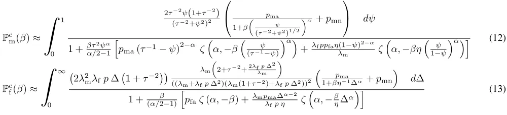
Theorem 1. The coverage probability in the macrocell tier is given in (12) (on top of next page), where ζ(a, b) =
2F1(1,1−2/a; 2−2/a;−b) is the Gauss hypergeometric
function.
Proof. The proof is given in appendix A.
2) Femtocell coverage:
Theorem 2. The coverage probability in the femtocell tier is given in (13) (on top of the previous page).
Proof. The proof is given in appendix B
B. Throughput
In this section, the throughput is defined for the BSs of each tier. The throughput in bps/Hz of each BS in the network is defined as a function of the coverage probability as
Ti= log2(1 +β)Pci(β), i∈ {m,f}. (14)
Now, depending on the load, the effective throughput (Tiu, i∈ {m,f}) experienced by a typical user in thei-th tier varies and the number of users that are served by the same BS needs to be taken into account. Thus, we now proceed to find the throughput achieved by the macro and femtocell typical users.
4As will be clear after the coverage probability analysis, we could easily
include the noise factor in the coverage probability at the cost of an extra integration.
1) Macrocell user throughput: The macrocell typical user throughput is presented in the next theorem.
Theorem 3. The macrocell typical user throughput is ex-pressed as
Tum≈
Z 1
0
T0 pum
pma
1 +β ψ
(τ−2+ψ2)1/2
α +pmn
× λ
mτ−2 λu
ln 1− λu
λmτ−2(B+τ2)
1− λu
λmτ−2B
!
fψ(ψ)dψ
(15)
where T0 = log2(1 + β) and B = 1 +
pmaβτ2ψα(τ−1−ψ)2−
α
ζ
α,−β
ψ (τ−2−ψ2)1/2
α
α/2−1 +
λfppfaβητ2ψα(1−ψ)2−α
λm(α/2−1) ζ
α,−βη1−ψψα+λuτ2
λm .
Proof. The proof is presented in appendix C.
2) Femtocell user throughput:
Theorem 4. The femtocell typical user throughput is expressed as
Tfu≈T0Pcf(β) λf λu
1−
1 + λu 3.5λf
−3.5!!
(16)
wherePcf(β)was previously defined in (13).
Proof. The proof is given in appendix D.
IV. ENERGYEFFICIENCY
In order to characterize the power consumed in the system, we make use of EARTH’s model [26] given as
Pi=
Pitx
ηP A i (1−σ
f eed i )
+PRF
i +PiBB
(1−σDC
i )(1−σiM S)(1−σCOOLi )
(17)
where ηP A
i is the efficiency of the power amplifier, PiRF
is the RF transmit energy consumption, PBB
i is the power
consumption of the base band interface,σif eedaccounts for the
feeder loses. Additionally, σDC
i , σM Si and σiCOOL represent
respectively the loss factor of the DC-DC power supply, main supply and cooling of the sites. The typical values of the components used in this work are presented in Table I. From (17) we see that the power consumption model agrees with the general model assumed in other works ( [27]–[29]) which considers a component (ai) dependent on the transmitted
power and a component (bi) independent of it. The power
consumption can then be expressed as
Pi =aiPitx+bi (18)
whereai=ηP A 1 i (1−σ
f eed
i )(1−σDCi )(1−σM Si )(1−σCOOLi )
andbi=
PRF i +PiBB (1−σDC
i )(1−σM Si )(1−σCOOLi ).
The EE is defined in terms of the throughput and the power used to operate the cellular system. We use the definition provided in the Energy Consumption Rating [30], as
EE= T
Pcm(β)≈
Z
10
2τ−2ψ(1+τ−2)
(τ−2+ψ2)2
pma
1+β
ψ (τ−2 +ψ2)1/2
α +pmn
dψ
1 +βτα/22−1ψαhpma(τ−1−ψ)2−α ζ
α,−β(τ−ψ1−ψ)
α
+λfppfaη(1−ψ)2−α
λm ζ
α,−βη1−ψψαi
(12)
Pcf(β)≈
Z
∞0
2λ2
mλfp∆ 1 +τ−2
λm
2+τ−2+2λfp∆2
λm
((λm+λfp∆2)(λm(1+τ−2)+λfp∆2))2
pma
1+βη−1∆α+pmn
d∆
1 +(α/β2−1)hpfaζ(α,−β) +λmpma∆ α−2
λfp η ζ
α,−βη∆αi (13)
x - coordinates (metres)
-1000 -500 0 500 1000
y - coordinates (metres)
-1000 -800 -600 -400 -200 0 200 400 600 800 1000
Rs Rs=!1 D
[image:8.612.64.564.62.176.2]r=ARs
Fig. 2: Model considered for the approximation. The green diamond represents the typical user located at a distance r=
ψRs from the serving MBS, where Rs is the Stienen radius
for the typical cell. The typical macrocell dominant interferer is located at a distance Rsτ−1 from the MBS located at the
origin. The distance between the user and the closest dominant MBS is denoted as D.
whereT is the throughput in bps, andP is the power used in the system in Watts. For the scenario analysed in this paper, the EE is given by
EE= NmpmaTm+Nfpfap Tf
NmPm+NfPf
= λmpmaTm+λfpfap Tf
λm(pmaPm+pmnbm) +λf(pfaPf+pfnbf)
(20)
where theEE is given in b/s/Hz and we used the substitution
Ni =λiA,i∈ {m,f}. It is important to notice that one of the
techniques for future deployment of HetNets which promises high savings in the overall EE of the systems is the sleep mode configuration in the different types of BSs. In order to quantize the extra savings in power consumption by equipping the BSs with sleep mode configuration, we assume that both MBSs and FAPs can turn off some of their components in a given time slot when they are not serving any users. Under this scenario, (20) transforms into
EEsleep= λmpmaTm+λfpfap Tf
λm(pmaPm+pmnpsm) +λf(pfaPf+pfnpsf)
(21)
whereps
i,i∈ {m,f}is the power consumed when the BS in
thei-th tier operates in sleep mode. Thanks to the breakdown of the power consumption in a BS provided in EARTH’s project, a sleep mode power consumption can be quantized by assuming that some components of a BS can be shut down to save energy when the BS does not have any users to serve. In particular for a non-active BS, the transmitted power is Ptx
i = 0Watts, and so there is no power consumed
in the power amplifier. Also, we assume that in the baseband interface, only the processor remains on. Finally, in the small signal RF transceiver, we assume that the transmitter part can be shut down and only the power related to the receiver remains turned on for reception. With this assumptions, the total power consumption in a BS of the i-th tier operating in sleep mode is expressed as
psi =
PRFsleep
i +P
BBsleep
i (1−σDC
i )(1−σM Si )(1−σCOOLi )
. (22)
The values for the power consumption of the small signal transceiverPRFsleep
i and the baseband interfaceP BBsleep
i when
a BS in the i-th tier is operating in sleep mode are derived from [26], and presented in table I.
With the expression for the throughput and the power consumption in each tier previously found, the overall system EE can be found. In the next section, the numerical results for the proposed model are presented.
V. NUMERICAL RESULTS
In this section, we: (i) validate the already developed framework, (ii) employ the developed analytical model in conjunction with Monte Carlo simulations to explore coverage, throughput and EE performances for the considered HetNet deployment, and(iii) we compare the results obtained via the Stienen model with a traditional PPP of a two-tier network where maximum expected SINR is used as the association
scheme [31]. The results are presented in figures 3 to 8. It is
worthwhile mentioning that in the simulations, for the case of the femtocell typical user (r > Rs) when we place a random
user at a distance r from the typical MBS (located at the origin) following a Rayleigh distribution as detailed in section III, if the value ofrexceeds the size of the typical MBS, we suppress this point and generate another one, until it is located outside the Stienen radius (r > Rs) but inside the typical MBS.
TABLE I: SIMULATION PARAMETERS
Parameter Value Description
λm, λf, λu 1.54x10−6,0,6.16 x 10−4, Density of MBSs, FAPs and users respectively
{1.54 x 10−5,3.08 x 10−5,4.62x10−5}
αm=αf=α 4 Path loss exponent
ηP A
m , ηmP A 0.388,0.052 Efficiency of the power amplifier in the macro- / femtocell
PRF
m , PfRF 10.9,0.4 RF transceiver power in the macro- / femtocell
PBB
m , PfBB 14.8,1.2 Baseband interface power in the macro- / femtocell
PRFsleep
m , P
RFsleep
f 5.1,0.2 Sleep mode RF transceiver power in the macro- / femtocell
PBBsleep
m , P
BBsleep
f 5,0.1 Sleep mode baseband interface power in the macro- / femtocell
σDC
m , σfDC 0.06,0.08 Loss factor of the DC-DC power supply in the macro- / femtocell
σCOOL
m , σfCOOL 0.09, 0 Loss factor of the cooling of site in the macro- / femtocell
σM S
m , σfM S 0.07,0.1 Loss factor of the main supply in the macro- / femtocell
σmf eed, σff eed 0,0 Loss factor of the feeder in the macro- / femtocell
τ 1/2 Stienen radius factor
[image:9.612.314.550.77.491.2]model the distribution of a random variable describing the position of the user outside the Stienen cell but inside the typical MBS coverage region. This follows from the variation of a Voronoi cell and its asymmetry with respect to its seed. By placing the user in this manner, this will of course have an effect on the distribution of ∆ in (38) and so the theory will differ from the simulations. However, as it will be seen in this section, the results are not greatly affected.
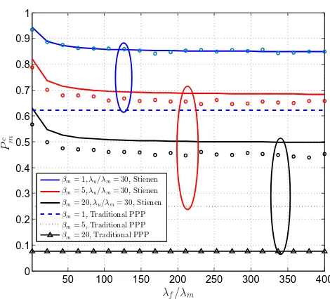
Fig. 3 shows the coverage probability in the macrocell tier, when the number of femtocells is increased in the service area. We can see that for small values of β the proposed model highly resembles the results found through simulations. Moreover, for a value of β = 20 the variation between the results from simulations and the analytical results is around
3%. Furthermore, we see that initially, increasing the number of femtocells deployed generates a decrease in the macro-cell coverage probability due to the increase of interference. However, when the number of femtocells deployed is large enough, the macrocell coverage probability reaches a constant value. Intuitively, these results follow from the fact that for a small density of FAPs, the coverage region of each femtocell is big, and so they will serve more users. By increasing the density, the coverage region of each femtocell decreases, and more FAPs will be active (i.e.,pfawill be higher) in order to
provide a service to the users located in the outermost areas of a macrocell. If the density of femtocells is high enough, the coverage region of each femtocell will be so small that it will only (approximately) serve one user. Therefore, the maximum density of active (interfering) FAPsλmax
f will equal
the density of users deployed in the femtocell tier coverage regions (i,e.λmax
f =λup). In other words, for a high number
of femtocells, the maximum number of interferers is dictated by the density of users.Additionally, the gains of the proposed model with respect to the traditional PPP two tier network with maximum SINR association scheme [31] are presented. Note that under this scheme developed in [31] it was shown that ignoring noise and using the same path loss exponent
(αm=αf =α), the coverage probability do not change with
the number of femtocells deployed, hence the straigh lines presented. A similar behaviour was found in [12] for some
50 100 150 200 250 300 350 400
0 0.1 0.2 0.3 0.4 0.5 0.6 0.7 0.8 0.9 1
λf/λm
P
c m
[image:9.612.318.553.267.480.2]βm= 1,λu/λm= 30, Stienen βm= 5,λu/λm= 30, Stienen βm= 20,λu/λm= 30, Stienen βm= 1, Traditional PPP βm= 5, Traditional PPP βm= 20, Traditional PPP
Fig. 3: Macrocell coverage probability (12) as a function of the density of femtocells deployed in the area for different threshold valuesβ, and λu
λm = 30. Circles represent the results from Monte Carlo simulations (with 5 x 10⁴ runs for each
point) while lines correspond to the analytical values.
specific cases.
In Fig. 4, we present the performance in terms of coverage probability for the femtocell tier, as a function of the fem-tocells deployed. We observe that increasing the number of femtocells in the area has a direct effect of increasing the coverage probability for a fixed value of λu and β. This
50 100 150 200 250 300 350 400 0
0.1 0.2 0.3 0.4 0.5 0.6 0.7 0.8 0.9 1
λf/λm
P
c f
[image:10.612.63.282.55.266.2]β= 1,λu/λm= 30, Stienen β= 5,λu/λm= 30, Stienen β= 20,λu/λm= 30, Stienen β= 1, Traditional PPP β= 5, Traditional PPP β= 20, Traditional PPP
Fig. 4: Femtocell coverage probability (13) as a function of the density of femtocells deployed in the area for different threshold valuesβ, and λu
λm = 30. Circles represent the results from Monte Carlo simulations (with 5 x 10⁴ runs for each
point) while lines correspond to the analytical values.
a MBS is expected to be low greatly improves the coverae probability of the femtocell tier, while the macrocell tier’s coverage is not highly affected. Note that by incorporating the strategic positioning of femtocells into the model, the coverage probability depends highly on the density of BSs. This is in contrast with results from other works which consider that all tiers are uniformly distributed in the area, in which case both the coverage and the data rates are independent of the density of BSs [12], [13], [31].Also from Fig. 4 we can conclude that only for a relatively small number of femtocells deployed, the traditional PPP achieves better results than those of Stienen’s model, but this trend is rapidly inverted as the number of femtocells increases.
In Fig. 5, the macrocell user throughput is presented as a function of the density of femtocells deployed in the area for the same threshold β and for different values of the density of users λu in the area. As expected, the increase in the
density of users reduces the throughput achieved per user in the macrocell tier. Due to the behaviour of the coverage probability, the throughput per macrocell user follows the same trend. Namely, by increasing the number of femtocells in the area, the throughput of the macrocell typical user is decreased until it reaches a minimum when the number of active interfering femtocells equals the number of users to be served by the femtocell tier.Comparing the results of Stienen’s model with the traditional PPP we can see that for a high enough number of femtocells, the traditional model achieves better results than Stienen’s model. However, these results are somehow misleading due to the fact that for a large number of femtocells the vast majority of users are being served by the femtocell tier. Moreover for the results in Fig. 5, when
λf
λm ≈ 130 (highlighted with the ellipses), the femtocell tier
50 100 150 200 250 300 350 400
0 0.2 0.4 0.6 0.8 1 1.2
λf/λm Tm
u
(b
p
s/Hz
)
βm= 5,λu/λm= 10, Stienen
βm= 5,λu/λm= 20, Stienen
βm= 5,λu/λm= 30, Stienen
βm= 5,λu/λm= 10, Traditional PPP
βm= 5,λu/λm= 20, Traditional PPP
βm= 5,λu/λm= 30, Traditional PPP
Fig. 5: Macrocell typical user throughput (15) probability as a function of the density of femtocells deployed in the area for the same value of β = 5, and for different values of the density of usersλu. Circles represent the results from Monte
Carlo simulations (with 5 x 10⁴ runs for each point) while
lines correspond to the analytical values.
will serve around 90% of the users, which will result in a
very inefficient macrocell deployment due to the high costs associated to the placement of MBSs. Moreover, similar gains are achieved by Stienen’s model in these cases.
The expected throughput per femtocell user is presented in Fig. 6 as a function of the number of femtocells deployed by keeping the same value for the threshold β and having different values of the user density λu. In these case, an
improvement in the perceived throughput per femtocell user is achieved by increasing the number of femtocells. These results provide the means by which network operators can plan the number of femtocells to be deployed in order to achieve a more balanced network in terms of the experienced user throughput. In other words, the operators can decide on the number of femtocells that would achieve the level of service required throughout the entire network, effectively eradicating the edge user bottleneck.Additionally, similar to the coverage probability, the femtocell user throughput in Stienen’s model rapidly surpasses the performance achieved by the traditional PPP with the increase in the femtocells deployed in the area. Note that in the proposed model, the coverage probability in the macrocell tier is over-estimated with respect to the simu-lations, while the macrocell user throughput is actually under-estimated. This is in contrast with the femtocell tier behaviour, where in general the femtocell tier coverage represents an under-estimation and the femtocell user throughput an over-estimation. This is due to the respective approximations made to simplify the analysis of both tier which have a different effect in the final approximations, namely, the interference ex-clusion region selection, and the assumptions of independence between the pairs of variables:rm with respect toRs, andrf
[image:10.612.321.551.58.262.2]50 100 150 200 250 300 350 400 0
0.5 1 1.5 2 2.5 3 3.5
λf/λm Tf
u
(b
p
s/Hz
)
β= 5,λu/λm= 10, Stienen
β= 5,λu/λm= 20, Stienen
β= 5,λu/λm= 30, Stienen
β= 5,λu/λm= 10, Traditional PPP
β= 5,λu/λm= 20, Traditional PPP
[image:11.612.322.547.57.267.2]β= 5,λu/λm= 30, Traditional PPP
Fig. 6: Femtocell typical user throughput (16) as a function of the density of femtocells deployed in the area for different threshold valuesβ, and λu
λm = 30. Circles represent the results from Monte Carlo simulations (with 5 x 10⁴ runs for each
point) while lines correspond to the analytical values.
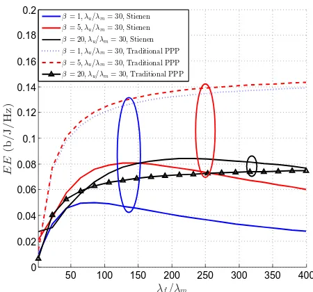
The EE of the network is presented in Fig. 7 when the num-ber of femtocells deployed is increased. We observe that the EE follows a quasi-concave shape, meaning that an increase in the number of femtocells is directly related to an increase in the EE of the network when the number of femtocells deployed is relatively small. However, as the number of femtocell increases beyond a given threshold (which varies with respect toβ), the EE of the system starts to decrease. This behaviour agrees with previous works on EE, where a trade-off between the achievable throughput (or spectral efficiency) and the EE has been observed. Intuitively, an increase in the number of femtocells deployed creates high gains in the expected throughput when this number is still relatively small. However, an increase in the number of FAPs deployed also generates an increase in the total power consumption of the network. As the achievable expected throughput is limited (given that the maximum value of Pc
f is 1), when the number of femtocells
deployed is significantly increased, the power consumed in all FAPs overweighs the increase in throughput and so the EE starts decreasing. This is evident from figures 4 and 7, where we can see for example that for β = 5 andλu = 30,
increasing the number of femtocells beyond λf
λm would give in an increase in the coverage probability, but it would also generate a decrease in the EE of the network.Also, in Fig. 7 it is shown that in general, the energy efficiency of the traditional PPP is higher than that of the Stienen’s model. However, this
highly depends on the values of β and λf selected, e.g. for
λf
λm = 400and β = 20 the EE achieved in both models is
very similar.
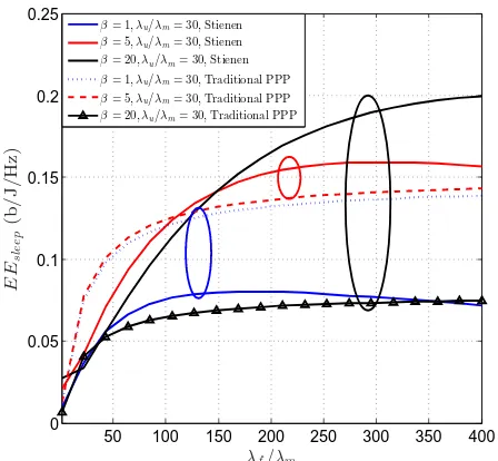
In Fig. 8, the EE of the network is plotted when both MBSs and FAPs have sleep mode capabilities. In this scenario, further improvements in the EE can be achieved by effectively turning
50 100 150 200 250 300 350 400
0 0.02 0.04 0.06 0.08 0.1 0.12 0.14 0.16 0.18 0.2
λf/λm
E
E
(b
/J
/Hz
)
β= 1,λu/λm= 30, Stienen
β= 5,λu/λm= 30, Stienen
β= 20,λu/λm= 30, Stienen
β= 1,λu/λm= 30, Traditional PPP
β= 5,λu/λm= 30, Traditional PPP
β= 20,λu/λm= 30, Traditional PPP
Fig. 7: EE (20) as a function of the density of femtocells deployed in the area for different threshold valuesβ, and λu
λm =
30.
off some components of the base stations in order to save power. We can see that even through the EE still follows a quasi-concave shape (as expected), the gradient with which the EE decays after reaching its maximum value is almost constant in comparison with the case without sleep mode. This gives the network operator more room to further increase the expected throughput while still having an acceptable performance in terms of the overall EE. Moreover, from Fig. 8 we observe an increase of about 87% in the maximum achievable EE with sleeping mode over the EE without sleeping mode for
β = 5 and λu
λm = 30.Additionally, we can see that including
sleep mode into the base stations in general results in a higher attained EE than the one obtained via the traditional PPP.
[image:11.612.64.285.57.264.2]50 100 150 200 250 300 350 400 0
0.05 0.1 0.15 0.2 0.25
λf/λm
E
Es
le
e
p
(b
/J
/Hz
)
[image:12.612.65.289.55.262.2]β= 1,λu/λm= 30, Stienen β= 5,λu/λm= 30, Stienen β= 20,λu/λm= 30, Stienen β= 1,λu/λm= 30, Traditional PPP β= 5,λu/λm= 30, Traditional PPP β= 20,λu/λm= 30, Traditional PPP
Fig. 8: EE with sleep mode capabilities (21) as a function of the density of femtocells deployed in the area for different threshold valuesβ, and λu
λm = 30.
to cope with the increase in traffic in particular areas.
VI. CONCLUSIONS
In this paper we introduced Stienen’s model for the mod-eling of non-uniform network deployment. With this model, femtocells are only deployed outside discs surrounding macro base stations. The radii depend on the distance to the closest MBS (and therefore depends also on each MBS size) which accounts for a realistic topology. Using stochastic geometry tools we found approximations for the coverage probability, expected user throughput and system energy efficiency of the network. Results confirm high gains in both throughput and the energy efficiency that can be achieved by cleverly placing femtocells in areas where the performance is expected to be low (near the edge of each MBS). Additionally, a more balanced network can be achieved, due to the fact that deploying a higher number of femtocells in the area with this topology greatly increases the femtocell user performance (users closer to the MBS edge) while the macrocell user performance is not significantly decreased.
As a result of the work undertaken in this study, a future direction consists of considering a non co-channel deployment between tiers can be considered. This way the inter-tier interference can be completely avoided. However, depending upon the number of users, there could be an underutilization of the available spectrum. Therefore, it would be interesting to study the interrelations between the BSs and user densities and their effect on the performance of the network in compar-ison with the joint channel deployment studied in this work. Additionally, the use of hybrid networks where a deployed ad-hoc network can make use of the cellular infrastructure has the potential to enhance the network performance. Therefore a case of interest would be in analysing the improvements of a hybrid network with a non-uniform deployment of femtocells,
where further improvements in network performance can be achieved and the inherent trade-offs between the performance of the ad-hoc and cellular components can be analysed.
APPENDIXA
PROOF OFTHEOREM1
From (11), the coverage probability in the macrocell tier is expressed as
Pcm=Erm
h
LΦm(s)|s=rα
mβLΦf(s)
s=rα
mβη
i
(23)
where η = Pftx
Ptx
m represents the ratio of the transmit powers employed by the tiers. Each Laplace transforms corresponds exactly to the probability generating functional of a PPP [3], which is defined as EQ
x∈Φf(x)
= exp(−λR
R2(1−
f(x))dx), where f(x) is a given function applied on each point of the process. For the considered scenario, the exact computation of the Laplace transform is not feasible. However, we obtain an approximation by following the approach taken in [32] for a fixed user location, and extend it for a random position in the service area. In Fig. 2 a sketch of the model used is presented. Under this scheme, the typical user which is located at a distance r from its serving MBS coincides withrm, and so we havefrm(rm) = 2πλmrmexp(−πλmr
2 m).
From Fig. 2, it is clear that the dominant interfering MBS is always located at a distance D from the typical user, and at a distance Rsτ−1 from the serving MBS, with Rs being
the Stienen radius of the typical macrocell. Therefore, the Laplace transform of the macrocell interference is decomposed into two components,Lm=LDm(s)L′m(s), whereLDm denotes
the Laplace transform of the interference form the dominant interfering MBS andL′
mdenotes the Laplace transform of the
interference from the rest of the MBSs. Additionally, we define a variable ψ = rm
Rs which corresponds to the ratio between the distance from the typical user to its serving MBS and the Stienen radius of that MBS. Using the law of cosines we obtain
D=p(Rsτ−1)2+r2m−2Rsτ−1rmcos(φ)
=Rs
p
τ−2+ψ2−2τ−1ψcos(φ)
≈Rs
p
τ−2+ψ2. (24)
whereφis the angle between triangle sides” Rsτ−1 and rm.
Due to the fact that the typical user’s position angle will be uniformly distributed, φwill also be uniformly distributed.
The Laplace transform of the interference from the domi-nant interfering MBS can then be evaluated as
LDIΦm(s) =EIΦm
h
exp (−IΦms)|s=rα
mβ
i
=E|h|2exp −s|h|2D−α
(a)
=E|h|2
"
exp −|h|2β ψ
(τ−2+ψ2)1/2
!α!#
= 1
1 +β ψ
(τ−2+ψ2)1/2
α (25)
where (a) was obtained using the substitution rm = ψRs.
probability pma and inactive with probability pmn, the final
expression is given as
LD IΦm =
pma
1 +β ψ
(τ−2+ψ2)1/2
α+pmn. (26)
As stated previously, the interference from the macrocell tier (other than the dominant interferer) is not symmetric with respect to the typical user. In this case, an approximation is obtained by considering that the interference to the typical user comes from outsideB xr, R
s(τ−1−ψ), wherexris the
position of the user. The Laplace transform of the interference from the other (not dominant) MBSs is then obtained as
L′
IΦm(s) =EIΦm
h
exp(−IΦms)|s=rα
mβ
i
=EΦm,|hj|2
exp
−s X
j∈Φm
|hj|2r−jα
=EΦm,|hj|2
Y
j∈Φm
exp −|hj|2β rαmrj−α
=EΦm
Y
j∈Φm
1
1 +βrj
rm
−α
(a)
≈exp
−2πλmpma
Z ∞
Rs(τ−1−ψ)
v dv
1 + v
β1/αψRs
α
(b)
=exp
−πλmpmaβ2/αψ2R2s
Z ∞
τ−1−ψ β1/α ψ
2
du
1 +uα/2
≈exp −λmπpmaβψ
α τ−1−ψ2−α
R2 s
α/2−1 ×
2F1
1,1− 2
α; 2−
2
α;−β
ψ
τ−1−ψ
α
.
(27)
where (a) is obtained by using the probability generating functional of a PPP [3] and (b) is obtained by using the
substitution u= rj
β1/αψR
s
2
. The Laplace transform for the interference from the femtocell tier is obtained by assuming a worst case scenario, in which the interference is assumed to come from outside B(x0, Rs(1−ψ)), and so the typical user
receives more interference than the one found in the scenario proposed. Considering this assumption, we have
LIΦf(s) =EIΦf h
exp(−IΦfs)|s=rα
mβη
i
=EΦf,|hk|2
"
exp −sX
k∈Φm
|hk|2r−kα
!#
=EΦf,|hk|2
" Y
k∈Φf
exp −|hk|2r−α k βη rαm
#
=EΦf
Y
k∈Φf
1
1 +βηrk
rm
−α
≈exp −λfπp pfaβ η ψ
α(1−ψ)2−α
R2 s
α/2−1 ×
2F1
1,1−2/α; 2−2/α;−βη
ψ
1−ψ
α
(28)
where the final expression is found by conducting a similar analysis as the one used for the macrocells. It is worth pointing out that in (11) the expression for the coverage probability requires averaging over rm and Rs. With the substitution rm = ψRs, the coverage probability can now be obtained
by taking the average overRs andψ. It is important to notice
that for the expression in (28), the distribution of ψ depends on the value ofRs. However, averaging over the conditional
distribution complicates the final expression. On the other hand, assuming independence simplifies the analysis and this approximation does not actually have a significant effect on the results (as will be evident in the results section), so we will use this approximation. We proceed to find the pdfs of these parameters, i.e., fRs(Rs)andfψ(ψ).
The pdf ofψis obtained by directly using the definition of the ratio distribution as
fψ(ψ) = Z ∞
0
Rs×fRs,rm(Rs, ψRs)dRs
= 2τ
−2ψ
(τ−2+ψ2)2. (29)
Finally, in order to effectively deal with the case when the user is served by the macrocell tier, we need to condition on the probability of the typical user being located inside the Stienen cell (pum=P(xr∈ B(0, Rs)), which is equivalent
to P(ψ < 1). From (29) it is straightforward to obtain
this probability as pum = 1 +τ−2 −1
. So the coverage probability in the macrocell tier is expressed as
Pcm(β)≈
1 pum Z 1 0 Z ∞ 0 LD IΦmL
′
IΦmLIΦf ×
fRs(Rs)fψ(ψ)dRsdψ. (30)
Substituting the values found in (29), (26), (27), (28) and (1) into (30) and integrating with respect to Rs, the final
expression in (12) is obtained.
APPENDIXB
PROOF OF THEOREM2
From (11), the coverage probability in the femtocell tier is expressed as
Pcf =Erf
h
LΦm(s)|s=rα
fβη−1 LΦf(s)
s=rα
fβ
i
. (31)
The Laplace transform for the femtocell interference in this case is assumed to be the same as in a normal PPP Voronoi but also considering the thinning of the density of interferers by a factor pfa accounting for the percentage of femtocells
Pcm(β)≈ Z ∞ 0 Z 1 0
2λmπψRs
τ 2
e−λmπR2s[ψ2+τ−2]
1−exp(−λmπR2s)
× LD IΦmL
′
IΦmLIΦf dψ dRs
Pcm(β)≈
Z ∞
0
Z 1
0
pma
1+β
ψ (τ−2 +ψ2)1/2
α +pmn
2λmπψRs
τ 2
1−exp(−λmπR2s)
×exp −λmπR2s
ψ2+τ−2
+pmaβψ
α τ−1−ψ2−α
α/2−1 2F1
1,1− 2
α; 2−
2
α;−β
ψ
τ−1−ψ
α
+λfp pfaβ η ψ
α(1−ψ)2−α
λm(α/2−1) 2F1
1,1−2/α; 2−2/α;−βη
ψ
1−ψ
α#!
dψ dRs
region). Therefore, the Laplace transform of the interference from the femtocell tier is given as
LIΦf(s) =EIΦf h
exp(−IΦfs)|s=rα
fβ
i
=EΦf
Y
k∈Φf
1
1 +βrk
rf −α ≈e
−λfπ pfaβR2s
α/2−1 2F1(1,1−2/α;2−2/α;−β).
(32)
For the macrocell tier interference, we note that the closest MBS (within the same Voronoi cell) now acts as an interferer, and it is always located at a distance rfrom the typical user, with the condition that r > Rs. Similar to the case of the
macrocell tier, we define a variable ∆ = rf
r that will help to
simplify the final expression for the coverage probability. With these considerations, we observe that the Laplace transform of the interference from the macrocell interference can once again be decomposed into two Laplace transforms, i.e.LIΦm =
Lr IΦmL
′′
IΦm, whereL
r
IΦm corresponds to the Laplace transform of the interference from the closest interferer (at a distancer, conditioned onr > Rs), andL
′′
IΦm is the Laplace transform of the interference from the other (non-closest interferer) MBSs. The Laplace transform of the interference from the closest MBS is given as
Lr
IΦm(s) =EIΦm
h
exp(−IΦms)|s=rα
fβη−1
i
≈E|h|2exp −s|h|2r−α
=E|h|2exp −|h|2βη−1∆α
≈ 1
1 +βη−1∆α. (33)
Considering that the closest MBS will be active with probability pma and inactive with probability pmn, the final
expression is given as
Lr
IΦm(s)≈
pma
1 +βη−1∆α+pmn. (34)
For the Laplace transform of the other macrocell interfer-ence, we observe that the interference can be as close asr= rf
∆
(withr > Rs). Therefore, we have
L′′IΦm(s) =EIΦm
h
exp(−IΦms)|s=rα
fβη−1
i
=EΦm,|hj|2
Y
j∈Φm
exp −|hj|2rαf β η−1r−jα
=EΦm
Y
j∈Φm
1
1 +βη−1rj
rf
−α
(a)
= exp
−2πλmpma
Z ∞
rf
∆
v dv
1 + v
β1/αη−1/αr
f
α
(b)
=e
−πλmpma(βη)
2/α r2 f
R
∞ (β ∆) 1/α∆−2 du
1+uα/2
=e
−λmπpmaβη−1 ∆α−2r2 f
α/2−1 2F1(1,1−2/α;2−2/α;−βη− 1∆α)
(35)
where(a) is obtained by using the PGF of a PPP, and ((b))
is obtained by using the substitutionu= rj
β1/αη−1/αr
f
2
.
Now, thanks to the use of the variable ∆ = rf
r previously
defined, the final expression for the coverage probability needs to be averaged over ∆ and rf by assuming independence of
these parameters like we did in the macrocell case. The pdf of
rf is directly obtained from the closest neighbour distribution
of a PPP considering a thinning with probabilitypas
frf(rf)≈2πλfp rfexp −πλfp r
2 f
. (36)
In order to obtain the pdf f∆(∆), we first need to obtain
the pdf of the distance to the closest MBS conditioned on
r > Rs. We will denote asR the random variable following
the Rayleigh distribution for the closest neighbour with the condition that it can only take values above Rs. As Rs
distribution. The pdf ofR can then be found as
fR(R) = Z R
0
f(R|Rs)f(Rs)dRs
= Z R
0
2πλmR e−πλmR
2
(2πλmτ−2Rse−πλm( Rs
τ )
2
)dRs
= 2πλmR e−πλmR
2
1−e−πλmτ−2R2. (37) Once the distribution of R is found, the pdf of ∆ can be obtained by means of the ratio distribution as
f∆(∆) =
Z ∞
0
R ×fR,rf(R,∆R)dR
= Z ∞
0
R × 2πλmR e−λmπR
2
1−e−πλmτ−2R2 ×
2πλfp∆R e−πλfp(∆rf)
2
dR
= 2λ2mλfp 1 +τ−2
∆×
λm 2 +τ−2
+ 2λfp∆2
((λm+λfp∆2) (λm(1 +τ−2) +λfp∆2))2
!
.
(38)
With the expressions previously obtained and conditioning on the probability of the user being served by the femtocell tierpuf = 1−pum, the femtocell coverage probability is given
by
Pcf(β)≈
1 puf Z ∞ 0 Z ∞ 0 Lr IΦmL
′′
IΦmLIΦffrf(rf)f∆(∆)drfd∆. (39) Substituting the values found in (32), (33), (35), (36) and (38) into (39) and integrating with respect to rf, the final
expression in (13) is found.
APPENDIXC
PROOF OF THEOREM3
In order to obtain the user throughput in the macrocell tier we use the definition in (14) but considering for the coverage probability calculation the other users served in the same macrocell as the typical user due to the fact that they share the available resources. We need to take into account the fact that the pdf of a cell is modified when it is conditioned on the user being inside [22]. We proceed to find the pdf fRˆs( ˆRs)
of the typical Stienen cell radius Rˆs, by noting that it is
a random truncated distribution which is conditioned on the eventr < Rs(typical user inside the Stienen cell). With these
considerations the pdf of the typical Stienen cell conditioned on the typical user being inside it is given as
fRˆs( ˆRs) = 1 pum
Z Rˆs
0 fRs|r
ˆ
Rs|r
f(r)dr
= 1
pum
Z Rˆs
0
2πλmτ−2Rˆse−πλmτ −2Rˆs2
×
2πλmre−πλmr
2
dr
=
2πλmτ−2Rˆse−πλmτ −2Rˆs2
1−e−πλmRˆs 2
pum .
(40)
OncefRˆs( ˆRs)is found, the throughput for the typical user
in the macrocell tier can be obtained by taking into account the other users to be served in the typical Stienen cell. By taking the definition of the coverage probability of the macrocell tier in (30), but considering the conditioned pdf of the Stienen’s radius (Rˆs) recently found, the throughput of the macrocell
typical user can be obtained as
Tum≈Eψ,Rˆs,num
"
T0
LD IΦmL
′
IΦmLIΦf
1 +num
!#
=Eψ T 0 pum × ∞ X
num=0
Z ∞
0
LD IΦmL
′
IΦmLIΦf
1 +num
!
fnum(num)
× fRˆs( ˆRs)d
ˆ
Rs
i
. (41)
Using the definitions of the Laplace transforms,fnum(num) andB, previously defined we have
Tum ≈Eψ
T0 pum pma
1 +β(τ−2+ψψ2)1/2
α +pmn
×
( ∞
X
num=0
Z ∞
0
2πλmτ−2(λuπ)numRˆs 2num+1
1 +num
×
e−πλmτ−2Rˆs 2
B−e−πλmτ−2Rˆs 2
(B+τ2)
dRˆs
)#
=Eψ T0 pum pma
1 +β(τ−2+ψψ2)1/2
α +pmn
×
( ∞
X
num=0
B−1
num+ 1
λu λmτ−2B
num
−
∞
X
num=0
(B+τ2)−1
num+ 1
λ
u λmτ−2(B+τ2)
num)#
=Eψ T0 pum pma
1 +β ψ
(τ−2+ψ2)1/2
α +pmn
×
λmτ−2 λu
−ln
1− λu
λmτ−2B
+ln
1− λu
λmτ−2(B+τ−2)
≈Eψ "
T0 pum
λmτ−2 λu
(
ln 1− λu
λmτ−2(B+τ2)
1− λu
λmτ−2B
!)#
.
(42)
Taking the expectation with respect to ψ in (42), we obtain the final expression in (15).
APPENDIXD
PROOF OF THEOREM4
We first derive the pdf (fy(ˆˆ y)) of the area (yˆ) of the Voronoi