The relative importance of macrophysical and cloud albedo changes for aerosol-induced radiative effects in closed-cell stratocumulus: insight from the modelling of a case study

www.atmos-chem-phys.net/17/5155/2017/ doi:10.5194/acp-17-5155-2017

© Author(s) 2017. CC Attribution 3.0 License.

The relative importance of macrophysical and cloud albedo changes

for aerosol-induced radiative effects in closed-cell stratocumulus:

insight from the modelling of a case study

Daniel P. Grosvenor1, Paul R. Field1,2, Adrian A. Hill2, and Benjamin J. Shipway2

1_{School of Earth and Environment, University of Leeds, Leeds, LS2 9JT, UK} 2_{Met Office, Exeter, UK}

Correspondence to:Daniel P. Grosvenor (daniel.p.grosvenor@gmail.com) Received: 14 November 2016 – Discussion started: 23 November 2016

Revised: 2 March 2017 – Accepted: 15 March 2017 – Published: 20 April 2017

Abstract. Aerosol–cloud interactions are explored using 1 km simulations of a case study of predominantly closed-cell SE Pacific stratocumulus clouds. The simulations in-clude realistic meteorology along with newly implemented cloud microphysics and sub-grid cloud schemes. The model was critically assessed against observations of liquid water path (LWP), broadband fluxes, cloud fraction (fc), droplet

number concentrations (Nd), thermodynamic profiles, and

radar reflectivities.

Aerosol loading sensitivity tests showed that at low aerosol loadings, changes to aerosol affected shortwave fluxes equally through changes to cloud macrophysical char-acteristics (LWP, fc) and cloud albedo changes due solely

toNdchanges. However, at high aerosol loadings, only the

Nd albedo change was important. Evidence was also

pro-vided to show that a treatment of sub-grid clouds is as im-portant as order of magnitude changes in aerosol loading for the accurate simulation of stratocumulus at this grid resolu-tion.

Overall, the control model demonstrated a credible abil-ity to reproduce observations, suggesting that many of the important physical processes for accurately simulating these clouds are represented within the model and giving some confidence in the predictions of the model concerning stra-tocumulus and the impact of aerosol. For example, the con-trol run was able to reproduce the shape and magnitude of the observed diurnal cycle of domain mean LWP to within

∼10 g m−2 for the nighttime, but with an overestimate for the daytime of up to 30 g m−2. The latter was attributed to the uniform aerosol fields imposed on the model, which meant

that the model failed to include the low-Ndmode that was

ob-served further offshore, preventing the LWP removal through precipitation that likely occurred in reality. The boundary layer was too low by around 260 m, which was attributed to the driving global model analysis. The shapes and sizes of the observed bands of clouds and open-cell-like regions of low areal cloud cover were qualitatively captured. The daytimefc frequency distribution was reproduced to within

1fc=0.04 forfc>∼0.7 as was the domain mean nighttime

fc (at a single time) to within1fc=0.02. Frequency

dis-tributions of shortwave top-of-the-atmosphere (TOA) fluxes from the satellite were well represented by the model, with only a slight underestimate of the mean by 15 %; this was attributed to near–shore aerosol concentrations that were too low for the particular times of the satellite overpasses. TOA long-wave flux distributions were close to those from the satellite with agreement of the mean value to within 0.4 %. From comparisons ofNddistributions to those from the

satel-lite, it was found that theNd mode from the model agreed

with the higher of the two observed modes to within∼15 %.

Copyright statement. The works published in this journal are distributed under the Creative Commons Attribution 3.0 License. This licence does not affect the Crown copyright work, which is reusable under the Open Government Licence (OGL). The Creative Commons Attribution 3.0 License and the OGL are interoperable and do not conflict with, reduce, or limit each other.

1 Introduction

In this paper we describe 1 km horizontal grid-spacing simu-lations of marine stratocumulus clouds nested within a global operational analysis framework that provides realistic me-teorological initial conditions and lateral boundary forcing. A grid spacing of this order bridges the gap between large eddy simulation (LES) and global model resolution, allow-ing larger domains than possible with LES, but the direct rep-resentation of more detailed processes than is possible with global models. We perform the first tests for stratocumulus of a newly implemented microphysics package that includes a detailed representation of the effects of aerosol upon clouds and a diagnostic cloud scheme. We use this model to examine the response of the cloud field to varying aerosol concentra-tions.

Stratocumulus clouds are the dominant cloud type in terms of area, covering over one-fifth of the Earth’s surface in the annual mean (Wood, 2012). They exert a strong net nega-tive radianega-tive effect that has a major impact on Earth’s radia-tive balance (Hartmann et al., 1992) and only a small change in their properties would have a large radiative impact (e.g. Latham et al., 2008). The albedo and the spatial coverage of stratocumulus clouds are affected by both their macrophys-ical and microphysmacrophys-ical properties, with aerosol potentially playing a key role in modulating both of these aspects. If this is the case, then the accurate representation of cloud– aerosol interactions would be needed in order to make ro-bust predictions about the response of stratocumulus to cli-mate change and anthropogenic aerosol changes. Further-more, since uncertainties in the representation of stratocumu-lus have been identified as one of the major sources of uncer-tainty in climate model predictions (Bony, 2005; Soden and Vecchi, 2011), it follows that the treatment of aerosol will in-fluence this uncertainty if the aerosol has a significant cloud impact.

Stratocumulus clouds are also important for numerical weather prediction (NWP) because they modulate the surface temperature through its influence on downwelling shortwave and long-wave radiation at the surface. Furthermore, their in-fluence on visibility is a major consideration for aircraft oper-ations. There is therefore a strong impact on both commercial and general public weather forecasts and applications.

For the climate system, the radiative impact of stratocu-mulus is strongly dependent on macrophysical properties such as cloud fraction or cloud liquid water path (LWP), which are likely to be heavily influenced by large-scale cir-culation and meteorological factors. However, microphysical processes can also influence the macrophysical cloud prop-erties, as well as having important radiative impacts in their own right. If all else is equal, i.e. a fixed liquid water con-tent (LWC), increasing the concentration of cloud conden-sation nuclei (CCN) leads to smaller droplets that in turn produce more reflective clouds (Twomey, 1977). The reduc-tion of droplet sizes is also associated with the suppression

of precipitation. Since this removes the main sink for wa-ter in a cloud, it was suggested that precipitation suppres-sion via increases in aerosol would increase LWP and cloud lifetime (e.g. Albrecht, 1989), an idea that has been backed up by LES modelling studies (Berner et al., 2013; Feingold et al., 2015; Ackerman et al., 2004, hereafter A04). However, A04 showed that this is only true for precipitating clouds; once precipitation had been suppressed, further aerosol in-creases led to cloud thinning (LWP decrease) via inin-creases in entrainment. Mechanisms for this effect are discussed in Bretherton et al. (2007) and Hill et al. (2009). Observation studies have also demonstrated a lack of LWP increase in ma-rine stratocumulus at high aerosol concentrations (e.g. Ack-erman et al., 2000; Platnick et al., 2000; Coakley and Walsh, 2002).

Changes in precipitation and LWP that result from changes in aerosol can also be accompanied by changes in cloud frac-tion (Stevens et al., 1998; Berner et al., 2013, hereafter B13). An example of this is the occurrence of pockets of open cells (POCs). POCs constitute regions of open cells with low cloud fraction in amongst high-cloud-fraction closed-cell regions (Wood et al., 2011a). It has been suggested that the enhancement of precipitation by reduced aerosol con-centrations can cause a transition between a state of closed and open cells within stratocumulus (Rosenfeld et al., 2006), which is then enhanced by a positive feedback mechanism that has been called the “runaway precipitation sink” (Fein-gold and Kreidenweis, 2002), whereby precipitation leads to a reduction in the available CCN. All else being equal, re-ducing CCN leads to larger drops that enhance the formation of precipitation, promoting the removal of more CCN. High-resolution idealised LES modelling supports this idea (B13) and shows that these processes occur at smaller spatial scales than can be captured explicitly by general circulation models (GCMs).

A compromise between LES and GCMs is a coarser-resolution (∼1 km) regional model that can simulate larger domains for the same or less computational cost as an LES. Regional models have the advantage over LES in that they are driven by meteorological analyses that can capture the relevant large-scale dynamic and thermodynamic structure, allowing results to be more easily compared to real ob-servations. Aerosol effects can also be considered relative to dynamical forcing or meteorology effects. However, we also note that many models have the ability to nest down from regional model resolution to LES resolution (includ-ing the one used in this study), although the computa-tional cost for high-resolution nests can be prohibitive for large domains. Techniques for the better coupling of (non-LES) atmospheric models to high-resolution LES nests (with non-periodic boundary conditions) now exist and have been shown to compare well to observations (e.g. Chow et al., 2006; Xue et al., 2014, 2016).

in-volved in marine stratocumulus. For example, Boutle and Abel (2012, hereafter BA12) showed that a mesoscale model with a 1 km grid spacing could capture closed-cell stratocu-mulus well, but they did not look at open-cell behaviour. Results from WRF-Chem at coarser grid spacings (9 km, Yang et al., 2011; 12 km, Saide et al., 2012; 14 km, George et al., 2013), where the representation of stratocumulus is re-liant on boundary layer parameterizations, have also shown reasonable agreement with observations. Whilst the coarser-resolution models may capture the general features of closed-cell stratocumulus, the simulation of open closed-cells is likely to be more difficult owing to the smaller size of the precipitating and updraft regions and the small scales over which aerosol– cloud interactions occur. It is unclear whether the combina-tion of boundary layer parameterizacombina-tions and microphysics schemes used in the coarser models will encapsulate the cor-rect response to aerosols.

In this paper we present results using a regional nested configuration of the Met Office Unified Model (UM). It is driven by realistic meteorology and includes a new micro-physics scheme called CASIM (Cloud AeroSol Interaction Microphysics; see Sect. 2.1.2 for details) designed to sim-ulate the processes important to aerosol–cloud interactions. Simulating a well-observed case allows the critical assess-ment of the model against a wide range of relevant observa-tions. By demonstrating that the model is capable of repro-ducing the observations, we can argue that the model cap-tures the important physics and will provide a reliable base-line for predicting the influence of aerosol on this stratocu-mulus cloud system.

Thus, we aim to address the following questions:

1. Can a regional model produce a realistic representation of stratocumulus clouds when compared to a diverse range of observations?

2. How do the modelled clouds respond to aerosol? 3. What is the relative importance of macrophysical and

cloud albedo changes for aerosol-induced radiative ef-fects?

4. What is the relative importance of the sub-grid cloud scheme?

2 Data and methods

For this case study we simulate a near-coastal region of the SE Pacific (see Fig. 1) for the period 12–14 November 2008, during which time mostly closed-cell stratocumulus clouds were observed. This period coincides with the VOCALS field campaign, which took place in this region and provided a variety of cloud, aerosol, and meteorological measurements made from airborne, ship, radiosonde, and buoy observa-tional platforms (Wood et al., 2011b). A variety of satellite

Figure 1.A map of the SE Pacific region with the 1 km model do-main shown as a black box. The colours show the orography over land and the sea-surface temperature over the ocean, both at the

res-olution of the global model (N512;∼39 km×26 km resolution at

the Equator for dx×dy). The black dot shows the location of the

RVRonald H. Brown(20◦S, 75◦W).

data are also available. Further details of the simulations and the observations used are now described.

2.1 Model details

Table 1.The model vertical grid spacing (dz) of the inner 1 km nest

as a function of height (z) for the boundary layer.

Model level z(m) dz(m)

1 2.50 2.50

2 13.33 10.83

3 33.33 20.00

4 60.00 26.67

5 93.33 33.33

6 133.33 40.00

7 180.00 46.67

8 233.33 53.33

9 293.33 60.00

10 360.00 66.67

11 433.33 73.33

12 513.33 80.00

13 600.00 86.67

14 693.33 93.33

15 793.33 100.00

16 900.00 106.67

17 1013.33 113.33

18 1133.33 120.00

19 1260.00 126.67

20 1393.33 133.33

21 1533.33 140.00

(SSTs) just offshore of the coast at the latitudes of the model domain, which reduce with distance offshore until just west of 80◦_{W when they start to increase again.}

The 1 km inner nest also employs 70 vertical levels, but with a lower domain top of 40 km and thus a higher vertical resolution. Table 1 shows that the vertical resolution near the top of the boundary layer for the inner nest (∼1–1.5 km) is around 100–140 m. The 1 km nest uses a rotated pole coor-dinate system whose equator is situated at the centre of the domain. A parametrized convection scheme is not required at high resolution since the model is likely to be convection permitting.

The global simulation uses the operational microphysics scheme based on Wilson and Ballard (1999), which is a sin-gle moment scheme in that it does not represent the num-ber concentrations of hydrometeors. For the 1 km nest runs we primarily use the newly implemented double-moment CASIM aerosol scheme that is described in Sect. 2.1.2. 2.1.1 A sub-grid cloud scheme

The recent previous studies of stratocumulus with the UM that employed high-resolution nests, e.g. BA12, used a sub-grid cloud scheme (Smith, 1990) that was linked to the Wil-son and Ballard (1999) microphysics scheme. The sub-grid cloud scheme parameterizes the variability in relative hu-midity (RH) that occurs in reality within a grid box, which may allow cloud to form even if the mean grid-box RH is below 100 %. This can be important for stratocumulus since

the presence of some liquid cloud water generates long-wave cooling at cloud top, which creates instability within the boundary layer. This drives turbulent overturning that can in turn create more cloud (i.e. a positive feedback).

When CASIM was implemented into the UM, it was done so with no sub-grid cloud scheme. In this configuration there was a large under-prediction in the amount of stratocumulus (see Sect. 3.2.2). Therefore, work was undertaken to imple-ment and adapt the Smith (1990) approach to allow it to work with a multi-moment bulk scheme such as CASIM. Details of this implementation are provided in Appendix A.

2.1.2 The CASIM microphysics scheme

CASIM is a new multi-moment microphysics scheme for the UM that includes the effects of aerosol upon clouds and vice versa. This provides enhanced capability over the old opera-tional scheme in which the cloud droplet concentration was constant throughout the domain.

As with other bulk microphysics schemes, the cloud and rainwater are separated into two hydrometeor classes. In each class the drop size distributions are described using a gamma distribution with a prescribed shape parameter and prog-nosed bulk mass and number concentration, i.e. double mo-ment cloud and rain (for details on the multi-momo-ment imple-mentation, see Shipway and Hill, 2012). In this study, ice mi-crophysics is not switched on since only warm clouds were present in the study area.

If a model grid box is deemed to be sufficiently humid by the above-mentioned cloud scheme, then cloud water con-denses and the number of droplets activated is determined us-ing the scheme described in Abdul-Razzak and Ghan (2000), which makes use of explicitly resolved vertical velocity, hu-midity, and aerosol properties to compute the number con-centration of droplets activated. Autoconversion of cloud droplets to rain and droplet accretion is based upon Khairout-dinov and Kogan (2000), and the self-collection of rain fol-lows Beheng (1994). Details on the testing of the warm rain microphysics parameterizations used in CASIM in an ide-alized framework can be found in Hill et al. (2015). The scheme includes an option for the sedimentation of cloud wa-ter; however, this is switched off for most of the runs in this paper. We discuss the effect of switching this on for some test runs in Sect. 4.2. The hydrometeor fall–speed relation-ship follows Shipway and Hill (2012). Table 2 summarizes the microphysical parameterizations used and Table 3 gives the constants used.

Table 2.CASIM microphysics scheme parameterization summary.

Parameterization Reference

Aerosol activation Abdul-Razzak and Ghan (2000)

Autoconversion of droplets to rain Khairoutdinov and Kogan (2000)

Accretion of droplets by rain Khairoutdinov and Kogan (2000)

Rain self-collection Beheng (1994)

concentrations can change locally due to convergence and di-vergence. Details of the aerosol concentrations used in the different runs of this work are given in the next section. CASIM includes the option of aerosol processing, which in-cludes activation scavenging; in-cloud mechanical process-ing into fewer, but larger aerosol particles (via collision coa-lescence); precipitation washout of both in-cloud and out-of-cloud aerosol; and evaporative regeneration. These processes can lead to an overall reduction in the aerosol available for forming cloud droplets. However, aerosol processing is not switched on for the runs in this work, but will be considered in a later paper.

2.1.3 Details on model runs and sensitivities

We have performed several model runs that are listed in Table 4. The run denoted as Old-mphys uses the old mi-crophysics scheme (Wilson and Ballard, 1999), which also uses the Smith (1990) sub-grid cloud scheme and has a fixed cloud droplet concentration of 100 cm−3. All of the other simulations use the CASIM microphysics. CASIM-Ndvar is the control aerosol case, where the accumulation soluble-mode aerosol has been chosen (the mass mixing ra-tio was set to 4.6×10−8kg kg−1, the number concentration to 3.8×109kg−1) to produce droplet concentrations that are in approximate agreement with those observed (see Sect. 3.2.1). CASIM-Ndvar-RHcrit0.999 is the same as the control run except that the sub-grid cloud scheme has been switched off in order to investigate its impact.

Aerosol sensitivity runs have been performed where the soluble accumulation mode aerosol mass and number have been reduced by factors of 10 and 40 (CASIM-Ndvar-0.1 and CASIM-Ndvar-0.025 respectively) and increased by a factor of 10 (CASIM-Ndvar-10). This range of aerosol concentra-tions creates clouds with droplet numbers that bracket the range observed during the VOCALS field campaign, as we will show in Sect. 3.2.1.

2.2 Observations

Data from a variety of instruments onboard several observa-tional platforms, including satellite, ship, and aircraft, have been used to validate the model. The data used (including er-ror estimates from the literature) are described in Appendix B and summarized in Table 5.

Table 3.The microphysical parameters used in the simulations for

the equations described in Shipway and Hill (2012).ρwis the

den-sity of water.

Cloud Rain

Moment description parameters

p1 0 0

p2 3 3

Size spectra parameters

µ 0 2.5

Mass–diameter parameters

cx π ρw/6 π ρw/6

dx 3 3

Fall–speed parameters

ax 3×107 130

bx 2 0.5

fx 0 0

gx 0.5 0.5

2.3 Cloud fraction definition

In this paper we choose to define cloud using an LWP thresh-old of 20 g m−2. The use of LWP makes comparisons be-tween model and satellite instruments simpler. A threshold value of 20 g m−2represents a conservative estimate of the lower limit of the microwave instruments used to observe LWP.

3 Results

3.1 General case study features from the observations Figure 2 shows snapshot satellite images from 13 November, including daytime maps of LWP andNdfrom GOES-10 and

Table 4.UM model runs. “Standard RH_crit” refers to the standard profile (listed in Table A1) of the RH_critparameter that is used within the sub-grid cloud parameterization (see Appendix A).

Model label Description

Old-mphys Old (3-D) microphysics, with standard RHcrit

CASIM-Ndvar (CONTROL) CASIM microphysics, variableNd, standard RHcrit

CASIM-Ndvar-0.025 CASIM-Ndvar with aerosol×0.025

CASIM-Ndvar-0.1 CASIM-Ndvar with aerosol×0.1

CASIM-Ndvar-10 CASIM-Ndvar with aerosol×10

CASIM-Ndvar-RHcrit0.999 CASIM-Ndvar with cloud scheme OFF

appear to be present at night. These regions could be con-sidered as POCs (pockets of open cells) since they constitute large regions of low-cloud-fraction open cells in amongst a region of otherwise closed-cell stratocumulus.

TheNdmap shows the presence of a large spatial gradient

with high Nd values near the coast and lowNd values

off-shore, which seem somewhat anticorrelated with LWP. This may indicate correlations caused by meteorology (e.g. two separate air masses), or it could be the result of aerosol feed-backs upon LWP (or a combination of the two). This bound-ary crosses the UM model domain, splitting it roughly into two halves in terms of LWP, with a low-LWP and high-Nd

re-gion to the NE and a high-LWP and low-Nd region in the

southwest.

3.2 Model validation and aerosol sensitivity 3.2.1 Droplet concentration distributions

Figure 3 shows probability density functions (PDFs) of the cloud droplet number concentration for a snapshot daytime period (14:00 LST on 13 November) for the inner nest of the model domain for both the model and GOES-10 satellite in-strument. Since the satellite provides a 2-D field ofNd, it is

necessary to make a 2-D field from the 3-D model data. This is done by takingNdat the height of the maximum LWC for

each model profile since this helps to avoid theNdfrom

spu-riously small LWC grid boxes from being included. For sim-ilar reasons, data points from both the model and the satellite are ignored if the LWP is less than 5 g m−2, but only after the modelNdand LWP data have been coarse-grained from their

native 1 km resolution to that of GOES-10 (4 km).

The observations from GOES-10 show that there is a two-mode PDF, with a two-mode of very low Nd (∼25 cm−3) and

one at 215 cm−3_{. This reflects the two different air masses}

that seem to be present, as discussed earlier (Fig. 2, i.e. a near-coastal air mass with high Nd and an offshore air

mass with low Nd). The models only capture one of these

modes ofNdsince a spatially uniform aerosol field was

ap-plied. However, it is conceivable that the low-Ndmode may

also be the result of aerosol removal within the precipitat-ing open-cell regions of the stratocumulus since this too can lead to very lowNdvalues (B13). Since aerosol processing

and scavenging is not switched on for these runs, the model will not capture the latter process. Using fixed aerosol con-centrations allows the exploration of the extreme high- and low-aerosol-loading scenarios without the complications of aerosol source functions and processing. This extra complex-ity will be explored in a later paper.

The control model (CASIM-Ndvar) has a Nd

distribu-tion that has a similar width (to within ∼15 %) to that of the higher-Nd mode observed by GOES-10, although

it has a higher frequency of the higher Nd values (above

275 cm−3). Despite this, the modal value is lower for the model (155 cm−3) than for the large mode of GOES-10 (215 cm−3), although the broadness of the model distribu-tion means that it still has large frequencies of data at the position of the GOES-10 modal value. Given the lack of sen-sitivity of the modelled clouds to increasing the aerosol by a factor of 10, it seems unlikely that the small differences between the modelled and observed large-Nd mode would

have a very large impact on cloud properties. The lack of a lower-Ndmode in the model could be more important. This

is explored through the sensitivity tests where we reduce the aerosol.

Figure 3 demonstrates that reducing the aerosol by factors of 10 and 40 (CASIM-Ndvar-0.1 and CASIM-Ndvar-0.025) decreases the mode values ofNdto 25 and 3.5 cm−3

respec-tively. The CASIM-Ndvar-0.025 case produces droplet con-centrations that are very low, with no values above 10 cm−3. This is consistent with the observations of ultra-clean re-gions that have been observed in the outflow rere-gions of POCs (Wood et al., 2011a) and so can be considered as a lower re-alistic bound for aerosol concentrations. The CASIM-Ndvar-10 case produces droplet concentrations of up to around 3000 cm−3, although with a 95th percentile of 1585 cm−3. Aircraft observations from the VOCALS field campaign reported maximum Nd values of around 400 cm−3 in the

vicinity of the coast at 20◦S (Zheng et al., 2011) over the whole campaign period; thus, the modelled Nd values in

the CASIM-Ndvar-10 case are somewhat higher than those likely to occur in reality for this region. However,Ndvalues

Figure 2.Snapshots of LWP (aandb, gm−2) andNd(c)for 13 November 2008.(a)and(c)show 13:57 LST (daytime, 18:45 UTC) from

the GOES-10 geostationary satellite at 4 km resolution.(b)Shows 01:42 LST (nighttime, 06:30 UTC) from the AMSR-E instrument that has

a lower resolution of 0.25◦(GOES-10 LWP andNdretrievals are probably not reliable at nighttime). Note the different colour scales. The

AMSR-E image has a region missing to the west due to the polar orbiting nature of the satellite and the limited swath width. Black regions

in the LWP plots denote those where LWP<20 g m−2, which we have chosen to define as cloud-free. The blue box shows the location of

the 1 km resolution model domain.

the upper bound of Nd values that are likely to occur

any-where on earth. We will show later (e.g. Sects. 3.2.2 and 4.2) that the exact value for the upper bound of aerosol concen-trations is not important given the lack of impact of aerosol on cloud properties as demonstrated by comparisons between the CASIM-Ndvar and CASIM-Ndvar-10 cases.

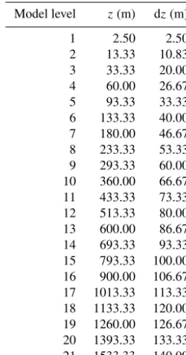
3.2.2 LWP and RWP time series

GOES-T able 5. Details on the observ ations used in this study . Instrument Measurements Product Product Nati v e pix el Estimated Reference used resolution resolution error Micro w av e radiometers (AMSR-E, SSMI–SSMIS, TMI, W indsat) L WP (liquid w ater path) Daily gridded 0.25 ◦ ∼ 37 × 28 km for lo west-resolution instrument 2–3 g m − 2 (Lebsock and Su , 2014 ) www .remss.com GOES-10 N d (droplet concentration) V OCALS re gion data set 4 km 4 km 20 % mean lo w bias, r = 0.91, RMSE = 36 cm − 3 (P ainemal et al. , 2012 ) W ood et al. (2011b ) GOES-10 L WP V OCALS re gion data set 4 km 4 km 14.7 % mean high bias, r = 0.84, RMSE = 26.9 g m − 2 (P ainemal et al. , 2012 ) W ood et al. (2011b ) CERES L W and SW T O A flux es SSF Le v el-2 snapshots 20 km 20 km 5 % for SW , 3 % for L W (Loeb et al. , 2007 ) http://ceres.larc.nasa. go v/products.php? product=SSF-Le v el2 Micro w av e radiometer (shipborne; stationed at 20 ◦ S, 75 ◦ W) L WP V ertical profiles ev ery 10 min n/a n/a Unkno wn Zuidema et al. (2005 ); de Szoek e et al. (2012 ) W -band (94 GHz) radar (shipborne; stationed at 20 ◦ S, 75 ◦ W) Radar reflecti vity (dBZ) V ertical profiles ev ery 10 min n/a n/a Unkno wn Moran et al. (2011 ), de Szoek e et al. (2012 ), F airall et al. (2014 ) n/a = not applicable

Droplet number concentration (cm )−3

Bin-normalized frequency

101 102 103

10−7 10−6 10−5 10−4 10−3 10−2 10−1 100

GOES, µ=136.1

CASIM−Ndvar, µ=173.7

CASIM−Ndvar−0.1, µ=23.7

CASIM−Ndvar−10, µ=612.5

CASIM−Ndvar−0.025, µ=5.2

Figure 3.PDFs of the cloud droplet number concentration for the model domain region. A snapshot time of 14:12 LST on 13 Novem-ber is used for the model and 13:57 LST for the GOES-10 satellite, which is the nearest available data point. Three-dimensional model

data are first converted to 2-D data, taking theNdat the height of the

maximum LWC with each model profile. The model data are subse-quently coarse-grained from their native 1 km resolution to that of GOES-10 (4 km). Data points from both the model and the satellite

are ignored if the LWP is less than 5 g m−2.

10 and the microwave instruments agree within∼10 g m−2_,

giving confidence in the observations.

The model runs produce the observed peaks and troughs in LWP and even capture the secondary peak on 13 Novem-ber at around 08:00 LST. The higher aerosol runs (CASIM-Ndvar and CASIM-(CASIM-Ndvar-10) and the old microphysics run (Old-mphys) also capture the magnitude of the LWP values well, although all simulations overestimate the daytime LWP values. There is better agreement for Old-mphys (overesti-mate of around 10 g m−2, or 10 %) than for the CASIM runs (overestimate of around 20–30 g m−2, or 50–75 %; however, note that the observed LWP is low at this time, being only 40 g m−2, resulting in a large percentage bias). The reverse is true for nighttime values where the CASIM runs match the observations very well (within 10 g m−2_{, or 10 %), but the}

Old-mphys run underestimates by 15–20 g m−2_{, or 15–20 %.}

Time (local solar time)

Liquid

water

path

(g

m

)

−2

LWP timeseries

12−Nov 06:00 12:00 18:00 13−Nov 06:00 12:00 18:00 0

20 40 60 80 100 120 140 160

AMSRE SSMI−f13 SSMI−f15 SSMI−f16 SSMI−f17 TMI Windsat GOES CASIM−Ndvar CASIM−Ndvar−0.1 CASIM−Ndvar−10 CASIM−Ndvar−0.025 Old−mphys

CASIM−Ndvar−RHcrit0.999

Figure 4.Time series of the mean LWP over the region of the UM domain for the different model simulations, the microwave satellite instruments, and the GOES-10 instrument. There are several microwave instruments that give snapshots throughout the diurnal cycle, as labelled in the legend; they are joined by the blue line. GOES-10 data are only used for the daytime, but they give higher time resolution.

Retrievals where the solar zenith angle is larger than 65◦have not been included due to likelihood of biases, as detailed in Grosvenor and

Wood (2014).

much of a precipitation suppression impact. This is demon-strated in Fig. 5 where rainwater path (RWP) is between 8 and 11 times lower in the control case than in the lowest-aerosol case.

CASIM-Ndvar-RHcrit0.999 is a model run where the sub-grid cloud scheme has been switched off, which results in a very large LWP reduction compared to the control case, with LWP values similar to those from CASIM-Ndvar-0.025 for the first day and CASIM-Ndvar-0.1 for the second day. The results clearly highlight that while it is possible for the aerosol environment to have a large impact on the struc-ture of the stratocumulus cloud deck (see CASIM-Ndvar-0.025 and CASIM-Ndvar), the role of the treatment of sub-grid humidity, even for sub-grid spacings of 1 km, is still as im-portant as a factor of 10–40 reduction in aerosol loading (see Ndvar and Ndvar-0.025 or CASIM-Ndvar-0.1). Given the unrealistically low LWP values in the CASIM-Ndvar-RHcrit0.999 case, the results from this run will not be included in future plots for clarity.

3.2.3 LWP maps and cloud coverage

Figure 6 shows the same daytime satellite LWP image from the GOES-10 satellite that was shown in Fig. 2, but zoomed in to the region of the model domain. Also shown are corresponding images from the control, very-low-and high-aerosol runs (CASIM-Ndvar, CASIM-Ndvar-0.025 and CASIM-Ndvar-10). The satellite image reveals that the clouds are orientated in diagonal-band-like structures of high LWP, and it also shows the structure of the POC regions, i.e. small regions of higher LWP (presumably the updraft region)

surrounded by regions of negligible cloud (downdraft–cold pool front region). There are two main POC regions within the model domain region: one centred at around 19.75◦S, 78.25◦_{W and another more elongated region centred at}

22.5◦_{S, 76.75}◦_{W, but stretching to the NW and SE.}

The control and high-aerosol simulations qualitatively rep-resent the diagonal band structures and the low LWP val-ues near the coast (in the NE corner of the domain) very well, despite the fact that there is no spatial gradient in the aerosol field of the model, as there would be in reality. This indicates a general dominance of the meteorological state over the macrophysical properties of the clouds. However, in the very-low-aerosol run (CASIM-Ndvar-0.025), LWP val-ues and the cloud fraction are significantly lower, indicating a cloud macrophysical response via the precipitation rate, which is similar to what has been observed in LES studies (Berner et al., 2013; Feingold et al., 2015). For the high-aerosol case, little impact of high-aerosol on the cloud field was found relative to the control case. This is because precipita-tion is low in the control case (Fig. 5) and so the addiprecipita-tion of more aerosol cannot influence precipitation.

Time (local solar time)

Rainwater

path

(g

m

)

−2

RWP timeseries

12−Nov 06:00 12:00 18:00 13−Nov 06:00 12:00 18:00 0

1 2 3 4 5 6 7 8 9

CASIM−Ndvar CASIM−Ndvar−0.1 CASIM−Ndvar−10 CASIM−Ndvar−0.025 Old−mphys

Figure 5.As for Fig. 4, except for RWP and for the models only.

Figure 6.Daytime snapshots of LWP (g m−2) for 13 November 2008 for the region of the inner model domain.(a)GOES-10 satellite at

13:57 LST (daytime);(b)model with control aerosol;(c)model with×0.025 aerosol;(d)model with×10 aerosol. The model images are

from 14:12 LST. Regions where the LWP is less than 20 g m−2are plotted as black to give an estimate of cloud fraction.

The nighttime LWP maps in Fig. 7 show that a large area of high-LWP cloud is observed by AMSR-E. The CASIM-Ndvar and CASIM-Ndvar-10 models also produce a large region of high-LWP cloud in the southwest corner of the domain, but this is less widespread than observed and reaches higher LWP values. As for the daytime, there is little response between the Ndvar and

CASIM-Ndvar-10 cases, but a large response when aerosol is reduced (CASIM-Ndvar-0.025), again with lower LWPs and lower cloud fractions that are similar to open-cell stratocumulus. 3.2.4 LWP distributions

Figure 7.As for Fig. 6, except for nighttime (01:42 LST for AMSR-E and 02:12 LST for the model).

(a)

(b)

Liquid water path (g m )−2

Bin-normalized frequency

LWP PDFs

0 100 200 300 400 500 0

0.002 0.004 0.006 0.008 0.01 0.012 0.014 0.016 0.018

REMSS, µ=106.1 CASIM−Ndvar, µ=120.8

CASIM−Ndvar−0.1, µ=89.8

CASIM−Ndvar−10, µ=123.0 CASIM−Ndvar−0.025, µ=45.7

Old−mphys, µ=106.4

Liquid water path (g m )−2

Bin-normalized frequency

LWP PDFs

0 100 200 300

0 0.005 0.01 0.015 0.02

REMSS, µ=51.5 GOES, µ=38.6

CASIM−Ndvar, µ=71.5

CASIM−Ndvar−0.1, µ=55.4 CASIM−Ndvar−10, µ=73.4

CASIM−Ndvar−0.025, µ=29.6

Old−mphys, µ=57.5

Figure 8.PDFs of LWP for daytime (left) and nighttime (right) time periods for the model and for satellite observations. “REMSS” refers to the several available REMSS microwave instruments, each of which provides a snapshot LWP field. For the daytime, the times surrounding the minima in the LWP diurnal cycle (see Fig. 4) are used (10:00–18:00 LST on both 12 and 13 November; overall four REMSS snapshots). For the nighttime, only the REMSS satellites are shown; times are chosen surrounding the maxima of the LWP cycle, but the surrounding period is reduced compared to the daytime in order to match the limited available REMSS times as closely as possible (03:00–09:00 LST on 12 November, 20:00 LST on 12 November to 10:00 LST on 13 November, 18:30–20:00 LST on 13 November; contains nine REMSS

snapshots). The model and GOES-10 data have been coarse-grained to the AMSR-E resolution of 0.25◦.

18:00 LST on 12 and 13 November) from both the REMSS microwave instruments (hereafter referred to as REMSS) and GOES-10. There is some disagreement between GOES-10 and REMSS, with GOES-10 generally producing more low LWP values (and fewer high ones). This could indicate

Liquid water path (g m )−2

Bin-normalized frequency

LWP PDFs ship for 12 Nov 06:00−14 Nov 00:00 UTC

0 100 200 300 400 500

0 0.005 0.01 0.015 0.02

Ship, µ=112.5

CASIM−Ndvar, µ=132.3

CASIM−Ndvar−0.1, µ=74.7

CASIM−Ndvar−10, µ=141.2

CASIM−Ndvar−0.025, µ=47.0

Old−mphys, µ=83.1

Figure 9. PDFs of LWP for the period from 06:00 UTC on 12 November to 00:00 UTC on 14 November 2008 from the RVRonald H. Brownmicrowave radiometer and various UM model runs. For both the ship and the model, 10 min averaged data are

used. For the model the 3×3 grid boxes centred at the location of

the ship (20◦S, 75◦W) are used and combined into one PDF in

order to account for the possibility of spatial variability.

good agreement with the observations, although frequencies are too low for the lowest LWP bin centred at 15 g m−2 and slightly too high for LWP values >∼60–100 g m−2, which is consistent with the overprediction of the mean LWP (Fig. 4). This is especially true when comparing to GOES. The CASIM-Ndvar-0.1 and Old-mphys runs are quite simi-lar to each other and both exhibit less underprediction of the low LWP values than the CASIM-Ndvar and CASIM-Ndvar-10 runs. The CASIM-Ndvar-0.025 run has too few high LWP points and too many low ones, again consistent with the un-derprediction of mean LWP for this run compared to the ob-servations.

Also shown are nighttime LWP PDFs from the REMSS satellites only. The models all show some degree of under-estimate for LWP values at around 130 g m−2and have fre-quencies that are too high at lower LWPs of around 30– 100 g m−2, but with the CASIM-Ndvar and CASIM-Ndvar-10 runs showing less overprediction than the other runs. As demonstrated for the daytime, the CASIM-Ndvar-0.025 run has a much larger number of low LWP values compared to the observations and the other models, indicating exces-sive LWP removal by precipitation. Consistent with this, the higher-aerosol runs (CASIM-Ndvar and CASIM-Ndvar-10) and the Old-mphys run have a small number of points with LWP larger than around 300 g m−2, which are not present for the low-aerosol runs (Ndvar-0.025 and CASIM-Ndvar-0.1). There are also higher frequencies of the higher LWP values in the CASIM-Ndvar-0.1 case compared to the CASIM-Ndvar-0.025.

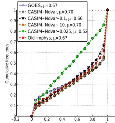
0.25o cloud fraction for LWP.GT.20 g m−2

Cumulative frequency

CF PDFs

−0.20 0 0.2 0.4 0.6 0.8 1 1.2 0.1

0.2 0.3 0.4 0.5 0.6 0.7 0.8 0.9

1 GOES, _{CASIM−Ndvar,} µ=0.67_µ=0.70 CASIM−Ndvar−0.1, µ=0.66 CASIM−Ndvar−10, µ=0.70 CASIM−Ndvar−0.025, µ=0.52 Old−mphys, µ=0.67

Figure 10. Cloud fraction cumulative distribution functions be-tween 08:12 and 16:12 LST for the model and 07:57 and 15:57 for GOES-10 sampled every 30 min. Here each cloud fraction value is calculated as the fraction of data points with LWP greater than

20 g m−2relative to the total number of data points in 0.25◦×0.25◦

areas. GOES-10 data are used at the native 4 km resolution and the model LWP data are first coarse-grained to this resolution from the native 1 km resolution.

In addition to spatial satellite PDFs, the microwave ra-diometer onboard the RV Ronald H. Brown can provide a measure of temporal variability at a resolution of 10 min, but at a fixed location (20◦S, 75◦W). Figure 9 shows LWP PDFs from the ship and for various model runs for the time pe-riod 06:00 UTC (01:12 LST) 12 November to 00:00 UTC on 14 November (19:12 LST on 13 November). A long sam-pling period is necessary given the restriction of the ship sampling being at only one location.

Figure 9 shows that all of the models underestimate the occurrence of LWP>150 g m−2 values and overestimate the occurrence of the lower LWP values for this region (LWP<50–100 g m−2depending on the model run). How-ever, the overestimate of the low values is much less severe for the CASIM-Ndvar and CASIM-Ndvar-10 runs. These re-sults are consistent with the REMSS nighttime rere-sults from Fig. 8.

3.2.5 Distributions of cloud fraction

Figure 10 shows distributions of cloud fraction (fc) for the

SW upwards TOA (W m−2)

Bin-normalized frequency

0 200 400 600 800

0 0.001 0.002 0.003 0.004 0.005 0.006 0.007 0.008 0.009 0.01

CERES µ=444.1 CASIM−Ndvar µ=378.4 CASIM−Ndvar−0.1 µ=245.4 CASIM−Ndvar−10 µ=431.6 CASIM−Ndvar−0.025 µ=158.1 Old−mphys µ=415.6

LW upwards TOA (W m−2)

Bin-normalized frequency

2600 270 280 290 300 310 320

0.01 0.02 0.03 0.04 0.05 0.06 0.07 0.08 0.09

CERES µ=278.5 CASIM−Ndvar µ=278.8 CASIM−Ndvar−0.1 µ=279.0 CASIM−Ndvar−10 µ=278.8 CASIM−Ndvar−0.025 µ=281.6 Old−mphys µ=277.1

(b)

(a)

Figure 11. Shortwave (left) and long-wave (right) top of the atmosphere radiative flux PDFs from CERES and the model for daytime periods for the region of the model domain. This is a combined PDF from the three separate snapshot overpass times of the CERES satellite for the model domain that were available for the simulation period: 10:24 LST (15:12 UTC) on 12 November (Terra satellite), 14:19 LST (19:06 UTC) on 12 November (Aqua satellite), and 11:07 am LST (15:55 UTC) on 13 November (Terra). For the model, the three closest available times were used: 15:00 and 19:00 UTC on 12 November 16:00 UTC on 13 November. Note that CERES–Aqua data are not available for the afternoon (local time) of 13 November. The model data were first coarse-grained to 20 km, which is the approximate resolution of the CERES data.

Figure 10 shows agreement between the model and ob-servations to within 0.1 in terms of cloud fraction for all of the runs, except for the lowest aerosol case (CASIM-Ndvar-0.025), suggesting that the model is very capable of correctly simulating the balance of cloudy and cloud-free areal cover-age. For the model runs (excluding the lowest aerosol case) and the observations, thefcbin that contributes most to the

frequency is the highest fc value (>0.95), corresponding

to nearly overcast conditions. The Old-mphys and CASIM-Ndvar-0.1 runs both have similar contributions to the fre-quency from this bin, as well as for other fc values at the

upper end of the distribution, with both underestimating the contribution to the total compared to the observations (i.e. these models do not have enough of the higherfc values).

In contrast, the CASIM-Ndvar and CASIM-Ndvar-10 agree with the observations to within ∼0.04 cloud fraction for fc>0.7. Thus, CASIM microphysics with the sub-grid cloud

scheme seem to represent an improvement over the old mi-crophysics in this aspect.

The low-aerosol case (CASIM-Ndvar-0.025) showed a much greater frequency of the lower cloud fractions and very few fully overcast data points, which is consistent with the re-sults and discussion of the snapshot maps (discussed above). A distribution plot is not possible for the nighttime where only coarse resolution (0.25◦) snapshots from the microwave instruments are available. The domain-average cloud frac-tion using the same 20 g m−2 LWP threshold was 0.95 for the AMSR-E satellite image (Fig. 7), which is very similar to that predicted in the control and high-aerosol cases (0.97 and 0.98 respectively after coarse graining to 0.25◦). Again, the very-low-aerosol case (CASIM-Ndvar-0.025) showed the

tendency to produce a much lower cloud fraction (0.79). Thus, the model shows large sensitivity of the cloud coverage to aerosol for the entirety of the daytime period and likely for the nighttime period too.

3.2.6 Radiative flux distributions

Figure 11 shows PDFs of the shortwave and long-wave top-of-the-atmosphere (TOA) fluxes from CERES and the mod-els for the region of the model domain (hereafter SWupTOA

and LWupTOArespectively). The results show that the aerosol

amount has a large influence on the shortwave (SW) fluxes, with the CASIM-Ndvar-0.1 and CASIM-Ndvar-0.025 runs showing mode fluxes that are much lower than those ob-served by CERES. The other runs produce SW distributions that are very similar to the those observed with CERES. The low values in the CASIM-Ndvar-0.1 run are unlikely to be the result of cloud fraction differences since Fig. 10 showed similar distributions for this and the higher aerosol runs. In-stead, the response of the SW flux results from the marked change in LWP when aerosol is changed (Fig. 4) and from the change inNd(Fig. 3); this attribution is discussed in more

The CASIM-Ndvar, CASIM-Ndvar-10 and Old-mphys runs all produce SW and LW distributions that are relatively close to those observed. There are a few discrepancies for the SW fluxes such as the observed peak in frequencies between 500 and 700 W m−2not being captured by the models, which show correspondingly larger peaks at lower SW values. PDFs of LWP and Nd at the specific

times of the SW CERES overpasses for the model and GOES-10 (not shown) suggest that the error is attributable to an underestimate in the number of Nd values between

around 210 and 300 cm−3. The Old-mphys run hasNdfixed

at 100 cm−3. For LW the Old-mphys run has values that are shifted slightly towards lower LW values compared to the other runs, which agrees with the observations better than the CASIM runs for the upper tail of the distribution, but not as well for the lower tail. The modal value of the CASIM runs is also slightly too high compared to the observations, whereas the mode for Old-mphys is slightly too low. The mean values of the CASIM-Ndvar, CASIM-Ndvar-0.1 and CASIM-Ndvar-10 runs agree with CERES within 0.2 %, with the Old-mphys and CASIM-Ndvar-0.025 runs perform-ing slightly worse (−0.5 and+1.1 % biases respectively).

Figure 12 shows the equivalent plot, but for nighttime snapshots. The models generally all produce distributions that are shifted to too-high LW flux values, indicating either clouds that are too low in altitude, cloud fractions that are too low, or clouds that are too thin. However, we note that cloud thickness would only be relevant for very thin cloud regions (<∼20 g m−2) since the increase in LW flux with LWP saturates at low LWP values (Miller et al., 2015). As for the daytime results, there is a much greater shift to high values for the CASIM-Ndvar-0.025 run, indicating the lesser cloud coverage in this case. The Old-mphys run is shifted to slightly lower values compared to the other runs as was also the case for the daytime LW fluxes. Again, Old-mphys agrees better than the other runs for the upper tail of the observa-tions, but not for the lower tail, which is representative of cloud top conditions.

3.2.7 Thermodynamic profiles

Regular radiosondes were released from the RVRonald H. Brown, allowing a comparison of the model to observations for thermodynamic profiles. Figure 13 shows this compari-son for the potential temperature (θ) and water vapour mix-ing ratio (qv) for the control run only (CASIM-Ndvar);

ex-cept forqvfor the CASIM-Ndvar-0.025 run, all of the runs

showed very similar results and so are not shown. CASIM-Ndvar-0.025 was likely anomalous due to the lack of cloud cover in that run. Three times are shown that are close to the peaks and troughs of the diurnal cycle of LWP (see Fig. 4), but excluding the first peak at 03:00 LST on 12 November to allow for model spin-up.

For the first time shown (15:55 LST on 12 November, i.e. daytime), theθ profile from the model matches that

ob-LW upwards TOA (W m−2)

Bin-normalized frequency

2600 270 280 290 300 310 320

0.02 0.04 0.06 0.08 0.1 0.12 0.14 0.16

CERES µ=274.2

CASIM−Ndvar µ=275.3

CASIM−Ndvar−0.1 µ=275.6

CASIM−Ndvar−10 µ=275.3

CASIM−Ndvar−0.025 µ=278.3

Old−mphys µ=273.5

Figure 12.As for Fig. 11, except for nighttime periods and for long-wave only. The times used for CERES are 22:35 LST (03:23 UTC) on 12 November (Terra satellite), 02:39 LST (07:27 UTC) on 12 November (Aqua satellite), and 01:44 am LST (06:32 UTC) on 13 November (Aqua). For the model, the three closest avail-able times were used: 03:30 and 07:30 UTC on 12 November; 06:30 UTC on 13 November.

served almost exactly, including the height of the sharp in-version, but theqvprofile is around 1 g kg−1too moist in the

boundary layer. The decrease inqvassociated with the

inver-sion is also not as sharp as in reality. The model biases for both of the other two times shown (13 November; nighttime, 03:29 LST; daytime, 15:09 LST) are similar to each other. In the model boundary layer, the modelledθandqvagree with

reality within 1 K and 0.5 g kg−1respectively, but the sudden changes associated with the inversion are too low by around 200 m. Above the inversion the model is also too warm by a maximum of around 3 K and slightly too moist in the region 500–600 m above the inversion by a maximum of approx-imately 1 g kg−1. Overall, the results suggest that the model matches reality very well in terms of the thermodynamic con-ditions, except for a tendency for the inversion to be too low by around 200 m.

3.2.8 Radar reflectivity

Potential temperature (K)

Height (m)

12−Nov−2008, UM = 15:42 LST, sonde = 15:55 LST

2800 300 320

1000 2000 3000

Sonde CASIM−Ndvar

qV (g kg−1)

Height (m)

12−Nov−2008, UM = 15:42 LST, sonde = 15:55 LST

0 5 10

0 1000 2000 3000

Potential temperature (K)

Height (m)

13−Nov−2008, UM = 03:42 LST, sonde = 03:29 LST

2800 300 320

1000 2000 3000

qV (g kg−1)

Height (m)

13−Nov−2008, UM = 03:42 LST, sonde = 03:29 LST

0 5 10

0 1000 2000 3000

Potential temperature (K)

Height (m)

13−Nov−2008, UM = 15:12 LST, sonde = 15:09 LST

2800 300 320

1000 2000 3000

qV (g kg−1)

Height (m)

13−Nov−2008, UM = 15:12 LST, sonde = 15:09 LST

0 5 10

0 1000 2000 3000

(a) (b) (c)

(d) (e) (f)

Figure 13.Profiles of potential temperature (top row) and water vapour mixing ratio (bottom row) from radiosondes released from the RV Ronald H. Brown (labelled “sonde”) and from the control UM run (CASIM-Ndvar). Three different radiosonde times are shown; 15:55 LST on 12 November (left), 03:29 LST on 13 November (middle), and 15:09 LST on 13 November (right), with the closest avail-able UM time being used (see titles of each sub-plot). The closest profile in the UM to the ship location is shown as the dashed grey line and

the surrounding thin grey lines show the 10th and 90th percentiles at each height from all of the profiles in a 1◦×1◦region around the ship.

region that surrounds the ship location to compute radar re-flectivity based on Rayleigh scattering. Tests using smaller sampling regions (down to 3×3 km; not shown) show very little change in the patterns of frequencies for the 2-D PDFs, indicating that the choice of sampling scale is not very impor-tant for this comparison. The ship radar results show a single mode of reflectivity up to values of around−4 dBZ that likely represent cloud droplets or small drizzle rather than larger rain droplets since model data in BA12 suggested that rain would appear as a separate mode at higher reflectivity values between around−10 and+10 dBZ. Most of the data points lie above 550 m in altitude, although there are some data from lower altitudes and there is a strong mode centred at 1135 m and−24 dBZ. The cloud reflectivity generally grows with altitude up to around 1 km, which is consistent with the growth of cloud droplets from above cloud base. Above this height the reflectivity starts to reduce; this could signify the evaporation of cloud due to the entrainment of dry, free tropospheric air into the upper regions of the clouds (A04), which could reduce reflectivity through changes in droplet size, number, or both. Alternatively, it may be the result of the presence of less drizzle near the top of the cloud. Most of the observed cloud is below 1325 m in altitude, although some cloud was observed up to 1460 m (within the accuracy of the height bins). It is likely that this corresponds closely with the boundary layer height because cloud tops for stra-tocumulus generally correspond with the inversion height.

The CASIM-Ndvar (control model) and CASIM-Ndvar-10 model results are similar to each other, but show some sig-nificant differences compared to the observations. The cloud from the model does not extend much above 1200 m, in con-trast to the observed cloud reaching 1460 m. This height dif-ference corresponds to approximately two model levels at these altitudes. Also, the model reflectivities do not tend to reduce with height towards the cloud top as they do in reality. The model also has a higher frequency of points at lower alti-tudes compared to the observations, e.g. the maximum height of the 3×10−3frequency contour is 693 m for the observa-tions and 293 m for the model. This leads to an overall cloud depth (as calculated using the frequency contour above) of 767 m for the observations and 907 m for the model (an 18 % overestimate). In the region of the lower-altitude cloud in the model, there is also a higher frequency of lower reflectivity values in the range−40 to−20 dBZ than is observed.

However, there are also some similarities; both the models and the observations show a general increase in reflectivity in the lower regions of the clouds, with a vertical gradient that is similar to that observed. Also, the highest dBZ values reached (99.9th percentile of all data, including cloud free re-gions) were around−5.2 dBZ for the observations, whereas for the model the equivalent values were −1.9, −6.7, and

CASIM-Figure 14.Two-dimensional relative frequency plot for radar reflectivity vs. height from the RVRonald H. BrownW-band radar and for var-ious model runs. The relevant model data are available every 30 min and data between the times of 06:00 UTC (01:12 LST) on 12 November and 00:00 UTC (19:12 LST) on 14 November are used, with the first 6 h of model data being avoided due to spin-up. Ship radar profiles are

available every 0.3 s and are used for the same time period as the models. Model data are used for the 1◦×1◦region around the location of the

ship. The colours indicate the normalized frequency of occurrence for each bin and the ship and model bin sizes are the same. Note that many

of the data points lie beyond the minimum value on thexaxis (i.e. very low radar reflectivity) and are not visible, but they are included for

the normalization. The ship radar has a minimum detectable reflectivity that increases with height; model data below this height-dependent

threshold were set to−1000 dBZ.

Ndvar-10 cases. In the CASIM-Ndvar-0.025 case the low aerosol concentrations allow larger droplets to form.

4 Discussion

A kilometre-scale regional model using cloud aerosol inter-acting microphysics has been used to simulate stratocumu-lus in the SE Pacific. It was seen that the introduction of the treatment of subgrid humidity (the cloud scheme) was im-portant for simulating the observations. The range of aerosol loading used in the sensitivity studies resulted in droplet con-centrations that included the observed range and captured ex-treme conditions for stratocumulus cloud. This provided in-sight into the relative importance of cloud brightening versus macrophysical changes such as cloud cover and LWP, which will be discussed further in this section.

4.1 Can a regional model produce a realistic representation of stratocumulus cloud when compared to a diverse range of observations?

We have shown that the UM regional model with the sub-grid cloud scheme reproduced many important physical observa-tions for the control case. The shape and magnitude of the observed diurnal cycle of domain mean LWP was captured to within∼10 g m−2for the control run for the nighttime, but with an overestimate for the daytime of up to 30 g m−2. The shapes and sizes of the observed bands of clouds were (qual-itatively) reproduced and the model simulated open-cell-like regions of low areal cloud cover to the NE of the domain and cloudy bands in the SW in between (Fig. 6). The daytime cloud fraction (fc) frequency distribution, especially for the

larger cloud fraction values (fc>∼0.7) was reproduced to

within a1fcof 0.04, as was the domain mean nighttimefcat

a single time (to within a1fcof 0.02). Frequency

value agreeing to within∼20 %. Also, the good comparison (to within∼15 %) of the width of the droplet concentration distribution indicates a good representation of model updraft velocities and the physics of the aerosol activation process, although we also acknowledge that the aerosol mass and number concentrations in the control model run were uni-formly scaled to approximately match the observed droplet concentrations.

Thus, there is good evidence that the model correctly cap-tures the physical processes that are of first-order importance for producing a realistic stratocumulus deck. However, there are some model deficiencies, which we now discuss, that were highlighted in the comparison to the observations.

Section 3.2.2 detailed how the daytime control run had a tendency to overestimate the LWP, particularly at the times of the lowest observed LWP. Examination of the daytime PDF of LWP (Fig. 8a) revealed a slight lack of LWP values be-tween around 15 and 70 g m−2 _{and too many of the higher}

LWP (>∼125 g m−2) values. A similar problem occurs at night (Fig. 8b), with a lack of LWP values between 150 and 250 g m−2and was also evident from the comparisons to the longer-term (day and night combined) single-location ship observations (Fig. 9). This overestimation of LWP may be related to the lack of a lower mode of modelledNdvalues,

which is evident from theNdPDF (Fig. 3). It is likely that

the presence of the low-Ndmode in reality caused LWP

re-moval through precipitation, which would lead to a reduction in the higher LWP values. The latter occurred in the lower-aerosol runs in the model (Ndvar-0.1 and CASIM-Ndvar-0.025), which were closer to the observed frequencies for the highest LWP values, and so if the lower-observed-Ndmode was present in the control model case (along with

the higher mode), then we would expect the match to obser-vations to improve. The dual mode ofNdthat was observed

in reality could have been the result of a spatial gradient in Nd(Fig. 2c), which is not captured by the model since we

employ a uniform aerosol field. The introduction of a spatial aerosol gradient or the use of a realistic aerosol model that simulates the aerosol sources, transport, and chemical trans-formation may rectify this problem.

BA12 found a similar daytime overestimate of LWP, but were only considering the near-coastal region where the ship was located. The reason for this was attributed to the sub-grid cloud scheme, which created too much cloud when sup-plied with the observed thermodynamic profiles. Since we use the same cloud fraction approach as BA12, albeit linked to a different microphysics scheme, this may also be an is-sue in this work. However, we note that the run with the old microphysics scheme (Old-mphys), which will be similar to the runs in BA12 since the same microphysics and cloud schemes are used, shows a domain-mean LWP value that is quite similar to that observed at the time of the daytime min-ima. This suggests that the overestimate in the near-coastal region that was observed in BA12 does not have a large im-pact on the overall domain mean. In addition, Fig. 4 clearly

shows that the aerosol concentration has an impact on the LWP at this time, with lower aerosol concentrations reduc-ing the LWP significantly.

Another issue with the model was that the cloud-top heights were too low compared to shipborne radar obser-vations (Fig. 14). This is consistent with the results from Sect. 3.2.7 and BA12 where the UM model boundary layer height was found to be too low for this case through com-parisons to radiosondes released from the ship, and it is also consistent with Abel et al. (2010) where the UM boundary layer height was on average∼200 m too low during the VO-CALS field campaign period for NWP configuration runs at 0.15◦resolution. BA12 found that an improved treatment of rain microphysics increased the height of the boundary layer in their 1 km resolution nest through the suppression of pre-cipitation. The improvements led to increased instances of coupled boundary layers as diagnosed by the boundary layer scheme. In our case, though, the boundary layer is too low even in the very-high-aerosol case (CASIM-Ndvar-10) when precipitation has already been completely suppressed, indi-cating that this is not the cause of the low boundary layer in our runs. The most likely source of this discrepancy is the meteorology of the global driving model, which imposes an initial capping inversion on the 1 km nest that is too low. This could be reinforced through the lateral boundary con-ditions, which might prevent the inner nest from growing its boundary layer through entrainment. Another possibility is that both the global model and the inner nest do not pro-duce enough entrainment, which then leads to boundary lay-ers that are too low. This is consistent with the results that are discussed in Sect. 4.2, whereby the modelled LWP in the high-resolution nest does not decrease at very high aerosol concentrations.

The fact that the modelled boundary layer height was too low is also consistent with the overestimate of the LW TOA upwards fluxes during both the daytime and the nighttime (Figs. 11 and 12) since it would correspond to cloud-top tem-peratures that were too large. It is possible that the LW TOA overestimate is also indicative of a cloud fraction that is too low, meaning that more surface points contribute. However, this seems less likely given that the cloud fraction generally agreed well with the observations during both the daytime and the nighttime, although we note that the nighttime com-parison of cloud fraction is limited to a single time.

4.2 How do the modelled clouds respond to aerosol? Figure 15 summarizes the response of various domain- and time-mean cloud properties to cloud droplet concentration (Nd), with theNdchanges being driven by aerosol changes.

The mean SWupTOA increases monotonically withNd with

the value for CASIM-Ndvar-10 being more than twice that in CASIM-Ndvar-0.025. The other cloud properties show a non-monotonic increase across all Nd values. Both the

domain-mean LWP and the in-cloud LWP (LWPic, cloudy

re-gions defined as LWP>20 g m−2) increase at lowerNd

val-ues with respectively 84 and 52 % increases between the CASIM-Ndvar-0.025 and CASIM-Ndvar cases when the aerosol was increased by a factor of 40. In contrast, there was very little increase in LWP between the CASIM-Ndvar and CASIM-Ndvar-10 cases when the aerosol was increased by a factor of 10.

This variation in response is due to the influence of aerosol on the suppression of rain. As shown in Fig. 15, at low Ndrain production (RWP) is relatively large; thus,

increas-ing aerosol leads to a reduction in rain production and an increase in LWP. When the mean Nd reaches around

200 cm−3(CASIM-Ndvar case), rain production has almost completely shut off; thus, any further increases inNdhave

no impact on LWP. Such behaviour is consistent with high-resolution LES studies (e.g. A04). The simulations presented here show that a coarser-resolution NWP model can simulate this behaviour. We also note that in some of the situations examined in A04, whenNdwas increased from very low to

high levels they simulated a similar proportional increase in LWP to that which we observe between the CASIM-Ndvar-0.025 and CASIM-Ndvar runs.

The simulations in A04 also showed that once precipi-tation had been completely suppressed, LWP tended to de-crease, with further Ndincreases due to entrainment effects

related to the ever-smaller droplet sizes (Bretherton et al., 2007; Hill et al., 2009). However, we do not see such be-haviour in our model in test runs (not shown) of the CASIM-Ndvar and CASIM-CASIM-Ndvar-10 cases that include droplet sed-imentation as a function of droplet size. This suggests that the entrainment parameterization within the boundary layer scheme (Lock et al., 2000) may need refinement to become more sensitive to the cloud droplet number concentration. Enhanced vertical resolution near the cloud top would also undoubtedly improve the explicit representation of the en-trainment interface layer, but such sensitivities are out of the scope of this study.

4.2.1 Cloud fraction response

Cloud fraction generally only increases between the CASIM-Ndvar-0.025 and CASIM-Ndvar-0.1 runs, indicating that the change in LWP between those runs is due to an increase in bothfcand LWPic. No major increase infcoccurs between

the CASIM-Ndvar-0.1 and CASIM-Ndvar cases, whereas

there is a fairly large increase in LWPic (27 %), indicating

cloud thickening.

Thus, the cloud fraction exhibits a step change, which only occurs at very lowNdvalues (mean values<30 cm−3in our

simulations). Such behaviour makes it questionable whether aerosol cloud metrics where the response of cloud fraction to Ndor aerosol is defined in terms of dlog(fc)/dlog(Nd)(e.g.

Quaas et al., 2010, albeit this study used aerosol optical depth instead ofNd) is appropriate, at least across a wide range of

Ndvalues. The addition of aerosol processing to our model

will alter this behaviour somewhat, with the likelihood be-ing that it will enhance the severity of the step change due to the positive feedback between CCN removal and precip-itation rate (runaway precipprecip-itation, B13). It may also shift theNdvalue at which it occurs to a higher value since small

amounts of precipitation at higherNd are likely to be

am-plified by CCN removal. Therefore, we expect open-cell re-gions to be more likely to occur with aerosol processing in operation.

4.3 What is the relative importance of macrophysical and cloud albedo changes for aerosol-induced radiative effects?

Since the impact on SWupTOA of stratocumulus is perhaps

the primary consideration, it is useful to break down the aerosol-induced changes in this quantity into separate re-sponses due to changes inNd(the cloud-albedo effect) and

changes in macrophysical cloud properties such as LWPic

andfc. A method for doing this using an analytical

calcu-lation of SWupTOAwith the time- and domain-mean model

cloud property values as inputs is described in Appendix C. Figure 16 shows the results, where the runs shown in Fig. 15 have been compared to the runs with the next highest aerosol concentration. The closeness of the red bars (changes in

SWupTOAbetween runs from the online radiation code) to the

totals from the value estimates using the analytical formulae suggest that the method works reasonably well.

The results indicate that the cloud-albedo effect (i.e. the change due toNdalone with LWPic andfc held constant)

plays a large role in causing the changes in SWupTOA seen

between the different runs, causing 44.5, 69.9, and 94.7 % of the total of the absolute changes (see Eq. C7) for the three comparisons made in Fig. 16. The contribution from Nd changes is largest for the comparison between the two

highest Nd runs since there is very little change in either

LWPic or fc for those runs. As Nd is reduced, the

contri-bution from changes in LWPicandfcincreases, but the

com-parison between the two lowest-Nd runs indicates that the

change due toNdis still the single largest factor. However,

given that changes to LWPic andfccan both be considered

macrophysical cloud responses and that there is some ambi-guity in the definition of LWPicandfcsince it depends on the

SW

↑

(W m

−2)

101 102 103

0 200

400 _{CASIM−Ndvar}

CASIM−Ndvar−0.1 CASIM−Ndvar−10 CASIM−Ndvar−0.025

LWP (g m

−2)

101 102 103

0 50

100 CASIM−Ndvar

CASIM−Ndvar−0.1 CASIM−Ndvar−10 CASIM−Ndvar−0.025

LWP

ic

(g m

−2)

101 102 103

20 40 60 80 100

120 CASIM−Ndvar

CASIM−Ndvar−0.1 CASIM−Ndvar−10 CASIM−Ndvar−0.025

RWP (g m

−2)

101 102 103

0

5 CASIM−Ndvar

CASIM−Ndvar−0.1 CASIM−Ndvar−10 CASIM−Ndvar−0.025

Droplet concentration (cm−3)

Cloud fraction

101 102 103

0.6 0.8 1

CASIM−Ndvar CASIM−Ndvar−0.1 CASIM−Ndvar−10 CASIM−Ndvar−0.025

Figure 15.Summary plots of domain- and time-mean quantities for the different model runs. The time average is weighted by the incoming SW TOA flux time series to give extra weighting to times when the cloud properties contribute to the SW flux, i.e. mainly in the daytime.

Thexaxis shows droplet concentrations, which are calculated in the same way as for Fig. 3. The top plot shows SW TOA flux, which is

followed by LWP (domain mean), in-cloud LWP (LWPic), RWP, and cloud fraction. Cloud fraction is calculated as for Fig. 10. Model data

at 30 min intervals between the times of 06:00 UTC (01:12 LST) on 12 November and 00:00 UTC (19:12 LST) on 14 November are used, with the first 6 h of model data being avoided due to spin-up.

change due to this combined macrophysical response would be 55.4 %, compared to 44.6 % for the cloud-albedo (Nd)

ef-fect, for the comparison between CASIM-Ndvar-0.025 and CASIM-Ndvar-0.1 suggesting that overall macrophysical re-sponses are at least of equal importance whenNdis low.

4.4 What is the relative importance of the sub-grid cloud scheme?

For these simulations we introduced a sub-grid cloud scheme, which was shown in Fig. 4 to have a significant effect on cloud properties, even at the 1 km 1x value used here. Domain mean LWP values with the cloud scheme switched off were lower than those of the CASIM-Ndvar-0.025 case (lowest-aerosol run) for the first half of the sim-ulation. They were higher for the second half, but were still lower than for the CASIM-Ndvar-0.1 case. Thus, the effect of the cloud scheme was comparable to that of large changes in the aerosol, which means that the inclusion of such a scheme within the UM is vital for the simulation of realistic marine stratocumulus clouds and therefore also for their response to aerosol. This may also be the case for other models at this resolution. Given the importance of the cloud scheme, it would be prudent to perform further investigation in fu-ture studies into the setting of the RHcritparameter (see

Ap-pendix A), or methods for deriving RHcritthat use, for

exam-ple, sub-grid turbulent kinetic energy.

4.5 Model resolution considerations

The credible simulation of closed-cell stratocumulus using a horizontal resolution (1x) of 1 km and a fairly coarse vertical resolution is consistent with previous results in the literature, for example BA12. Close matches to observations have also been reported, using even coarser resolutions of 9 km (Yang et al., 2011) and 14 km (George et al., 2013) with the WRF-Chem model, albeit with the representation of stratocumulus relying heavily on the boundary layer–stratocumulus param-eterizations employed.

However, it is likely that a1xof 1 km or greater will not fully resolve some important effects, especially for cases that involve smaller-scale eddies such as open-cell cases where aerosol removal and cold pool dynamics associated with nar-row precipitating regions become more important. Model resolution also affects the spectra of vertical velocities that are represented, which has been shown to have an impact on the number of aerosol particles that are activated into droplets (e.g. Malavelle et al., 2014), and it also has dynamical impli-cations.