representations.
White Rose Research Online URL for this paper: http://eprints.whiterose.ac.uk/109702/
Version: Accepted Version
Article:
Cohen, Dale and Quinlan, Philip Thomas orcid.org/0000-0002-8847-6390 (2016) How numbers mean : Comparing random walk models of numerical cognition varying both encoding processes and underlying quantity representations. Cognitive Psychology. pp. 63-81. ISSN 0010-0285
https://doi.org/10.1016/j.cogpsych.2016.10.002
[email protected] https://eprints.whiterose.ac.uk/
Reuse
This article is distributed under the terms of the Creative Commons Attribution-NonCommercial-NoDerivs (CC BY-NC-ND) licence. This licence only allows you to download this work and share it with others as long as you credit the authors, but you can’t change the article in any way or use it commercially. More
information and the full terms of the licence here: https://creativecommons.org/licenses/
Takedown
If you consider content in White Rose Research Online to be in breach of UK law, please notify us by
Running Head: How Numbers Mean
How numbers mean: Comparing random walk models of numerical cognition varying both
encoding processes and underlying quantity representations
Dale J. Cohen1*, Philip T. Quinlan2
1
University of North Carolina Wilmington.
2
The University of York.
Words: 12273
Key Words: Numerical Cognition, Random Walk, Numerical Distance, Physical Similarity, Numerical Architecture, Simulation
*Correspondence to: Dale J. Cohen, Ph.D., Department of Psychology, University of North Carolina Wilmington, 601 South College Road, Wilmington, NC 28403-5612. Email: [email protected]. Phone: 910.962.3917. Fax: 910.962.7010. This work supported by NIH
Abstract
How numbers mean: Comparing random walk models of numerical cognition varying both encoding processes and underlying quantity representations
Understanding how numerical symbols and their associated quantities are represented and used is a primary aspiration of those working in numerical cognition. Once we understand how symbols are represented and assigned meaning, we will understand how best to frame questions about how organisms become numerate (Cantlon, Platt, & Brannon, 2008; Feigenson, Dehaene, & Spelke, 2004), how numeracy changes over time (Geary, 1994), how and why numerical errors arise (Macaruso, McCloskey, & Aliminosa, 1993), how language and numeracy are related (Hauser, Chomsky, & Fitch, 2002), whether or not numeracy is a cultural universal (Dehaene, Isard, Spelke, & Pica, 2008), and, so on. Despite almost half a century of
experimental study, the underlying representation of numerical symbols remains hotly debated. Here, we present a model of number symbol encoding, representation, and retrieval. We instantiate this model in a random walk simulation and predict performance in the core paradigm in the field of experimental numerical cognition: the relative quantity task. Although we
specifically simulate performance in the relative quantity task, the actual model informs more generally about how a number conveys the quantity it denotes. Indeed, the processes that we use to simulate performance in the task may reflect on more fundamental properties of the human perceptual system. Such general implications of the work are examined in detail later.
The relative quantity task
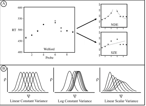
Yurko & Hu, 1981; Moyer & Landauer, 1967), to paradigms that include priming components (Dehaene, Naccache, Le Clec, Koechlin, Mueller, Dehaene-Lambertz, et al., 1998; Ratinckx, Brysbaert & Fias, 2005; Van Opstal, Gevers, De Moor & Verguts, 2008), Flanker components (Notebaert & Verguts, 2006), multiple dimensions (e.g., in numerical Stroop tasks; Pavese & Umiltˆ, 1998; Ratinckx & Brysbaert, 2002; Tzelgov, Yehene, Kotler, & Alon, 2000; Waldron & Ashby, 2001), and, so on. Nevertheless, the reaction time (RT) data from the relative quantity task, and its variations, have revealed two effects that have proved foundational in all subsequent theory development; these are the numerical distance effect and the size effect (see Figure 1A). The numerical distance effect is characterized by RTs (for correct responses) that monotonically decrease as the numerical distance between the two digits increases. The size effect is that, for a fixed difference between two digits, correct RTs increase monotonically as the size of the digits increase.
Moyer and Landauer (1967) conducted the classic experiment that identified the
numerical distance effect and size effects. The authors presented two Arabic digits, side-by-side, and asked participants to identify as quickly and accurately as possible the numeral denoting the larger quantity. Moyer and Landauer (1967) explained the numerical distance effect and size effect by proposing that numbers are represented as magnitudes that are similar to those in the physical world and the discriminability of two perceived magnitudes is determined by the ratio of the actual magnitudes (i.e., these representations obey WeberÕs law).
digit is represented on an internal continuum (e.g., an internal Ònumber line,Ó Dehaene, 2003) and there exists some perceptual variability (i.e., noise) associated with the placement of the digit on this continuum. Take, for example, the number Ò5.Ó All theories assume that each time an observer experiences this symbol, the observer will have a slightly different ÒsenseÓ of the quantity associated with Ò5.Ó So, sometimes the observerÕs sense is more than 5 and sometimes less. Accordingly, each digitÕs quantity representation is captured by a distribution of values on the continuum that we term a psychological distribution of quantity (PDQ) (see Figure 1B). The PDQ captures the perceptual noise associated with oneÕs understanding of the quantity associated with a digit. The PDQs of successive digits are rank ordered and overlap (see Figure 2).
In Signal Detection Theory, the degree of difficulty in distinguishing between two stimuli is determined by the amount of overlap between their corresponding perceptual distributions: the greater the overlap, the more difficult it is to distinguish between the two stimuli. This premise translates directly when discussing number representation. Most accounts explaining the psychological representations of numbers, assume the difficulty in distinguishing between the quantities of two numbers is determined, primarily, by the amount of overlap between their PDQs (see Figure 2). ÔDifficulty,Õ in this context, is defined by greater RTs and errors in the relative quantity task.
Theory (see Church, Meck & Gibbon, 1983; Gallistel & Gelman, 1992; Meck & Church, 1983; Meck, Church & Gibbon, 1985). The Logarithmic Theory also posits that the different PDQs have the same variance, but claims that the means of the ordered PDQs are spaced on a logarithmic scale. As such, the means of successive PDQs get closer together as the numbers increase (see Figure 1B). In contrast, for the Scalar Variance Theory, the means of the ordered PDQs are spaced linearly but their variances scale linearly (i.e., increase) with quantity (see Figure 1B).
In the absence of providing a detailed model, intuitions about general patterns of performance suggest that the numerical distance effect can be accommodated by all three theories because the PDQs of numerals denoting adjacent quantities (e.g., Ò5Ó and Ò6Ó) overlap more than the PDQs of numerals denoting distant quantities (e.g., Ò5Ó and Ò1Ó). It is similarly apparent that the Logarithmic Theory and Scalar Variance Theory accounts can accommodate the size effect. The size effect is hypothesized to result because, for a given quantity distance (e.g., Ò1Ó) the PDQs of numerals denoting large quantities (e.g., Ò7Ó and Ò8Ó) overlap more than the PDQs of numerals denoting small quantities (e.g., Ò2Ó and Ò3Ó). For the Logarithmic Theory this is true because the means of the PDQs for successive smaller quantities are farther apart than those for successive larger quantities. For the Scalar Variance Theory this is true because the SDs of the PDQs for successive smaller quantities are smaller than those for successive larger quantities. On first glance, though, the size effect sits less well with the Linear Theory.
details of models of this task from encoding to response, (ii) simulating data based on the specified details, and, (iii) and assessing the model fits against human data.
Modeling
When assessing the internal representation of stimuli, perceptual, decisional, and
response processes influence the participantÕs behavior. It is, therefore, vital to specify precisely the foundational assumptions about how each of these might influence the data. Without a precise specification, one may erroneously conclude that particular patterns of data are the result of internal representations, when in reality they are the result of encoding or decision processes (e.g., Verguts, Fias, & Stevens, 2005).
Traditionally, the cognitive systems involved in completing a simple RT discrimination task are described in terms of four broad stages, namely, Encoding, Comparison, Decision, and Response (see Sternberg, 1998). When explaining RT data, the researcher must ask critical questions about each stage: for instance, does the time to complete this stage correlate
significantly with the variable of interest? If the answer is ÒNo,Ó then the time resulting from that stage is assumed to contribute merely a constant across all levels of the independent variable, so the researcher can effectively ignore that stage when explaining the data. If, however, the answer is ÒYes,Ó then the researcher must include detailed discussion of the stage in explaining the data. Often, to simplify interpretation, researchers will assume that stages do not correlate with their variable of interest.
size effect would no longer be as simple as described. For example, suppose the response function is logarithmic or that encoding times are related to numerical distance. Such findings would undermine the current interpretations of the numerical distance and size effects. Thus, whereas simplifying assumptions can make data interpretation relatively straightforward, they can also lead researchers down a garden path. Below, we describe the potential influences of each of the four broad processing stages on performance in the relative quantity task.
Encoding
In the relative quantity task, encoding refers to the processes involved in converting and identifying the numerical symbol. As can be inferred from traditional explanations, encoding time has been assumed to be unrelated to numerical distance. Recently, however, Cohen (2009, 2010) has demonstrated that encoding of numerical symbols takes measurable time and this time is related to numerical distance.
In an effort to assess whether numerical symbols automatically activate their quantity representation, Cohen (2009) conducted a numerical same/different task. Here, the participants were presented with Arabic digits ranging from 1-9 and had to judge whether the digit presented was a 5. Theoretically, participants can complete the numerical same/different task based solely on the physical features of the numeral. Nevertheless, previous research using the numerical same/different task had revealed a function that correlated with numerical distance (Dehaene & Akhavein, 1995; Ganor-Stern & Tzelgov, 2008). Because numerical distance was task
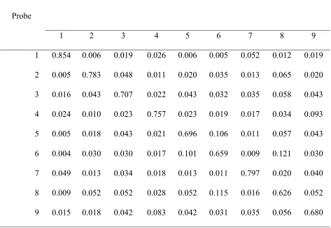
of the physical similarity of Arabic digits (PSdigit) based on the seven-line segment, figure 8 structure of digits used on digital alarm clocks:
PSdigit = O/D (1)
where PSdigit is the measure of physical similarity, O is the number of lines that the two integers share, and D is the number of remaining lines (see Table 1). Although the RTs were well fit by measures of numerical distance, the Physical Similarity function predicted the data virtually perfectly. Furthermore, when both numerical distance and physical similarity were entered into the equation, numerical distance dropped out leaving only physical similarity as the significant predictor. Cohen concluded that, although numerical distance is an important predictor of RTs when quantity information is either required to complete the task (e.g., a relative quantity task) or when quantity is an inherent part of the task (a numerical Stroop task), integers do not
automatically activate their quantity representation. Importantly, physical similarity correlated at over .6 with numerical distance. Cohen (2009) explained this correlation as likely resulting from the fact that Arabic digits evolved from analogue representations of the quantities themselves. Therefore their physical form would be correlated with numerical distance. In a later paper, Cohen (2010) showed that physical similarity was the primary predictor of RTs in a relative quantity task that used decimals presented in Arabic notation. Since CohenÕs work, others have replicated the physical similarity effect with other languages and other paradigms (see Garc’a-Orza, Perea, Mallouh, & Carreiras, 2012).
cannot be avoided by presenting numerical symbols in two different formats (e.g., Ò5Ó vs. ÒsixÓ), because the numerical cognition system will automatically convert and compare symbols in a common representational system rather than comparing quantities.
Comparison
The comparison stage is the most well described stage of the cognitive processes
involved in completing the relative quantity task. This stage requires a description of the internal representation of quantity so that the relevant features to be described are understood. As
discussed above, all major theories accept a general signal detection framework, whereby the psychological quantity associated with this symbol is best described as a distribution with a mean perception and some variance around the mean (i.e., the PDQ). In turn, the similarity of the quantities denoted by symbols is described by some measure of the overlap of their respective PDQs. Signal detection theory provides numerous such measures, including dÕ, area under the curve, etc.
When comparing quantities, the time to complete a comparison is assumed to be some function of the overlap of the PDQs. Because the overlap of PDQs is determined solely by their relative mean placement and variance, these two features of the psychological representation of quantity are of critical importance. How best to characterize the internal number system in these terms, is the topic of a very heated debate. The debate rages over the relative strengths and weaknesses of the Linear Theory, Logarithmic Theory, and Scalar Variance Theory (although predominantly concern has been with the latter two, e.g., Cantlon et al., 2009; Dehaene et al., 2008). Having already provided a general description of these models, a more precise
Logarithmic Theory: ψi = log(Θi) + ei, ei~ N(0, s), (2) Linear Theory: ψi = Θi + ei, ei~ N(0, s), (3) Scalar Variance Theory: ψi = Θi+ ei, ei~ N(0, Θi * s) (4)
where the subscript i identifies the specific numerical symbol represented, ψ is the psychological quantity representation, Θ is the quantity denoted by the numerical symbol, and e represents the error variance.
The fixation with the Logarithmic Theory and Scalar Variance Theory in the literature results primarily from consideration of the size effect. That is, the data show that it takes longer to make a relative quantity judgment for larger numerals (e.g., 8 vs. 9) than for smaller numerals (e.g., 1 vs. 2). The Logarithmic Theory explains this effect by proposing that the means of the PDQs of successive integers are distributed logarithmically rather than linearly. So, the means of the PDQs of small numbers are farther apart than the means for the PDQs of large numbers. In contrast, the Scalar Variance Theory explains this effect by proposing that the variance
associated with the PDQs for large numbers is larger than the variance associated with the PDQs for small numbers. In both cases, the PDQs overlap more for larger than for smaller numbers. These functions appear to accommodate the size effect.
The Linear Theory model does not accommodate the size effect in the comparison stage. This, however, is not necessarily a fatal problem. It is possible that the size effect is a
manifestation of another stage (e.g., encoding or response), but such a hypothesis has not been seriously considered or tested by those advocating the Logarithmic Theory or Scalar Variance Theory. We return to this possibility later in the paper.
Modeling the decision and response stages of an RT task requires an underlying theory of decision-making. Virtually all well described models of RTs are based on a Signal Detection Theory model of decision-making very similar to the one used to describe the comparison process (e.g., Ashby, 2000; Curtis, Paulos, & Rule 1973; McGill, 1963; Ratcliff, 1978; Thomas & Myers, 1972). Thus, we can borrow from what has been learned about the link between RTs and Signal Detection Theory in order to address issues about numerical cognition.
Many of the successful models linking Signal Detection Theory and RT make the RT-Distance assumption. For example, Thomas and Myers (1972) presented a mathematical analysis of RT on the assumption that RT is a monotonically decreasing function of the Euclidean
distance between the percept and the criterion as described in Signal Detection Theory. Ashby and Maddox (1994) called this the RT-Distance hypothesis (see Ashby & Maddox, 1994). Thomas and Myers (1972) elaborated their account by (i) specifying the form of the RT
distribution given that part of the variation in RT is the result of distance to criterion, and, (ii) by accepting that, for any fixed distance, RT is a random variable with a non-degenerative function. The authors continued by clarifying predictions on the form of the RT probability curve,
variance, and mean of the RT distributions under various assumptions. Thomas and Myers (1972) concluded that the experimental data fit the predictions well. In following up on this work, Balakrishan and Ratcliff (1996) presented evidence that participants will use a distance to criterion rule when assigning confidence ratings even when the optimal decision rule is different. Furthermore, Zakay and Tuvia (1998) showed that confidence ratings and choice RT are
Most detailed computational models of the relation between RT and the underlying psychological representation are variants of the Random Walk model (Link, 1990). The random walk model assumes a Signal Detection framework. Although the Random Walk model can generalize to more than two distributions, we will describe a simple two alternative forced choice procedure. Here, the participant is presented two stimuli and must identify one as the correct choice with the push of a button. The participantÕs RT is recorded. Let us specify that the task is a relative quantity task and the participant is to choose the number symbol that denotes the largest quantity. Here, the Random Walk model assumes that each number symbol (say Ò4Ó and Ò5Ó) activates separate PDQs.
To estimate RT, the model will repeatedly sample from both PDQs and find their
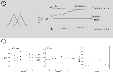
difference (see Figure 2). So, for example, on the first sample, the model will randomly select a value from the PDQ representing 4 and may retrieve a 3.5 (recall that the quantities associated with the number Ò4Ó is noisy, so error occurs). Similarly, the model will randomly select a value from the PDQ representing 5 and may retrieve a 6. Here, the difference between the selected values is 2.5 (6-3.5 = 2.5). So, on the first sample the model moves 2.5 units in the positive direction. On the next sample, the difference is added to the previous sample. The Random Walk model takes repeated samples until the sum of all the sample differences passes a pre-determined threshold. The positive threshold indicates that the participant responds that the Ò5Ó is greater than the Ò4.Ó The negative threshold indicates that the participant responds that the Ò4Ó is greater than the Ò5.Ó Importantly, the number of samples required to pass the threshold is taken as the surrogate for RT.
erroneously passing the incorrect threshold, thus leading to an error. The number of samples taken before encountering a boundary is a function of the shape, variance, and degree of overlap of the perceptual distributions, and is assumed to be a monotone function of RT.
Buckley and Gillman (1974) were amongst the first to generate a random walk model of performance in timed numerical comparison tasks. They accepted a standard Signal Detection Theory model and assumed that the transformation from external stimulus to internal
representation was logarithmic. In one comparison task that they described, two digits (taken from the set 1-9) were presented side-by-side and participants responded whether the left or right was the larger. Buckley and Gillman (1974) conducted a standard random walk simulation and stated that this basic model was successful in being able to capture scaled time measures of the responses in the task. However, as pointed out by Link (1990), the simulated data were not the actual condition mean RTs but rank ordered mean RTs. Moreover, in the actual experiment, any trial that was responded to incorrectly was repeated until a correct response was collected. In this respect, the simulated data were error-free. As Link (1990) remarked this was regrettable
because one of the strengths of random walk models is their ability to model error data. In addressing these issues, Link (1990) explored the degree to which random walk
processes are able to simulate performance in variants of the speeded relative magnitude task. In one case, two-digit numbers were presented sequentially and the participant had to respond whether or not the current number was the larger or smaller than the immediate previous one. In a second case, a standard of 55 was used and participants simply had to respond whether a singly presented two-digit number was greater or less than the standard. Link (1990) carefully
validity and then used it to estimate model parameters that would mimic properties of the data in these tasks. Notably, Link accepted the Linear Theory representation but had to embellish his model with further ad hoc assumptions about (i) the nature of response bias, and, (ii) a numerical transformation in which the base 10 number system was mapped to a base 6 number system. Moreover, critically he did not assess the fit of competing theories of quantity representations on both correct and error data. In this regard, the work fails to provide further insights into how best to adjudicate between the key competing models as outlined above.
Two further modeling studies are notable. The first, by Poltrock (1989), examined how well random walk models could account for performance in a variant of the speeded magnitude estimation task (i.e., respond to the left or right digit that was the larger). In extending the experiments, participants were also tested under conditions where strict RT deadlines were imposed. Individual participantÕs RT and accuracy data were fit with a random walk model in which values of 10 free parameters were estimated. The model resulted in peculiar estimates when comparisons involved the digit Ò1Ó. Essentially, the model predicted no distance effects if the digit Ò1Ó was included in the analysis. That is, if the data from the digit Ò1Ó was included in the analysis, the model estimated that the underlying quantity representations for all digits were equal distance from one another. However, if the digit Ò1Ó was excluded from the analysis, distance effects emerged that revealed that the estimated internal magnitudes of the remaining digits was approximately linear. No detailed account of this inconsistency was included in the paper.
was less than or greater than 5). Smith and Mewhort (1998) carried out extensive studies of diffusion random walk models in which participantsÕ performance was fit with two free parameters that defined Gaussian and ex-Gaussian parts of participantsÕ RT distributions. Simulations provided estimates of these parameters and these were then compared with the actual behavioral data. The models produced impressive fits with the correct RT data. Comparisons were also reported between the modelsÕ error data and human accuracy. The authors, however, did not model the error RT as a function of numerical distance. Rather, the authors calculated a single, omnibus, mean RT for error data, and showed that by adding variability to the start position of the walk they were also able to model how fast errors arise. Thus, similar to previous researchers, Smith and Mewhort (1998) modeled correct RTs while sidestepping the importance of modeling error RTs.
In sum, there is a strong tradition in which variants of a random walk process to model performance in speeded magnitude estimation tasks have been explored (see e.g.,
Kamienkowski, Pashler, Dehaene & Sigman, 2011; Schwarz, 2001; Sigman & Dehaene, 2005). The positive outcomes of this work indicate the utility of this approach. However, to date, researchers have not provided comprehensive models that account for the distributions of correct
and error RTs, as well and the proportion of errors1. As will become clear, it is only by
attempting such a comprehensive exercise, that differences between the various models become apparent and their relative strengths and weaknesses are laid bare.
The Current Models
Here we instantiated each of the three primary theories of quantity representation (Linear Theory, Logarithmic Theory, and Scalar Variance Theory) as, respective, computational
relative quantity task. The actual behavioral data were taken from a speeded relative quantity task in which participants were asked to judge whether a visually presented Arabic digit denoted a quantity greater than or less than five (described in detail below). An overarching aim was to be able to model these data comprehensively. Consequently, each of the models was required to produce estimates of both the speed and accuracy of response. The main objective was to go beyond previous modeling attempts in being able to fit the skew of the RT distributions for both the correct and incorrect response and the incidence of errors for each of the comparisons. Furthermore, we compared the performance of models with and without encoding processes. In addition, further analyses were directed towards comparing fits only for correct RTs and
comparing more comprehensive fits for both correct and error RTs. As such, we can clarify the significance of modeling encoding processes and we underscore the importance of assessing fits to complete data sets.
the size of the increment in the walk and the sign of this distance determines the direction of the walk.
To simulate a trial, one sample value was drawn from the perceptual distribution (ψ) of the standard and one from the probe and a running total of the difference between the two samples was logged, namely:
totj = totj-1+SQj Ð PQj, (5) where totj is the running total for sample j,SQj is the standard quantity drawn on sample j, and
PQj is the probe quantity drawn on sample j. A response was then initiated when totjcrossed a pre-specified decision threshold. If totj crossed the positive decision threshold, the standard was identified as being larger than the probe. If totj crossed the negative decision threshold, the probe was identified as being larger than the standard. The number of samples required (termed
NumSamp) prior to crossing a decision threshold was the dependent measure taken to be analogous to RT.
In our random walk model, the decision threshold is identified by three free parameters,
that instantiate two response biases. The first free parameter, ba, identifies the intercept of the
positive decision threshold. ItÕs negative value, -ba, identifies the intercept of the negative
decision threshold. These values represent the initial amount of evidence that the observer requires before he or she responds. The farther away these points are from 0, the more evidence required. We also incorporated linear, time-varying boundaries (Smith, 2000; Zhang, Lee, Vandekerckhove, Maris & Wagenmakers, 2014). That is, we allowed each boundary to be angled toward the Ò0Ó evidence line (between 0 and -50 degrees). As will become clear, it proved critical to incorporate such time-varying boundaries, in order to obtain best fits. The
threshold. Its negative value, -bq, identifies the angle of the negative decision threshold.
Although we assume the positive and negative decision thresholds are symmetric, this
assumption is not necessary. A functional consequence of incorporating these kinds of linear, time-varying boundaries is that a decrease in response evidence is required as time increases. In essence, this instantiates the increasing impulse to respond as time increases. Linear, time-varying boundaries have the effect of reducing the skew of the distributions, as well as influencing the relative means of error and correct RTs, as well as the proportion of errors. Finally, we assume between trial variance exists in the decision threshold angle. This third
decision threshold free parameter, bs, captures this variance. Thus, for any simulated trial, we
assume the threshold angle to be distributed as follows:
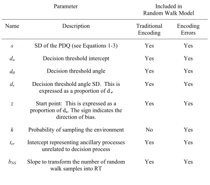
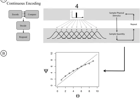
�~�(�&, �() (6) We ran two versions of the random walk model: one that included no encoding effects (termed the TraditionalEncoding model) and one that included encoding effects (termed the
Encoding Errors model). The Encoding Errors model assumes that the percept of the digit might be misperceived. This misperception will influence the perceived quantity and thus the
probe as a particular stimulus, we converted the similarity values of all the digits to proportions by presented probe3. Table 1 shows these probabilities. The sum of the perceived stimulus proportions for each presented probe (i.e., the rows) will sum to 1 (which is not the case when computed column-wise).
The Traditional model assumes no encoding errors as described above. The Encoding Errors model is as follows. The Encoding Errors model assumes that the Arabic digit is encoded before comparison, but the digit may be confused (Ò5Ó perceived as Ò6Ó). Here, prior to the random walk, the perceived probe is selected on the basis of the probability structure presented in Table 1. For example, if the presented probe was Ò3Ó then there would be a 5.8% chance of Ò8Ó being Òperceived.Ó Then the random walk simulation runs as if the perceived stimulus (e.g., 8) was presented.
Conventionally, researchers assume that encoding occurs once (in an all-or-none fashion) at the beginning of the process (e.g., Sternberg, 1998). We call this the initial encoding of the presented probe. We believe, however, that it is likely that the system continuously samples the environment. Such a system would, over time, correctly encode a stimulus that was initially mis-encoded. We included this potential correction process in our model. Thus, the Encoding Errors model assumes the visual system repeatedly samples the environment, with the result that slightly different impressions are derived at each time point. This information is continually made available to the magnitude comparison stage. Critically, every time the environment is sampled, the encoding of the probe is selected on the basis of the probability structure in Table 1 and a quantity is sampled from the encoded digitÕs PDQ.
� ������ = 100�5, (7)
where k is a free parameter ranging from 0-1 indicating the strength of the first encoding. If k = 0, then the initial encoding carries all the information and there is no further encoding. If k = 1, then there is 100% probability of a new encoding every sample of the Random Walk. Here, the perceived probe will change on every sample independent of the previous sample. If 0 < k < 1, then the probability of a new encoding decreases exponentially with every step of the Random Walk. The second parameter, n, is the sample number of the Random Walk (starting at 0).
For steps in which the system does not interrogate the environment, the system must use a memory representation to identify the PDQ from which the Random Walk will draw the next sample. When k = 0, then that representation is the initial encoding. When k > 0, then the system uses the most frequently encoded integer since the initial encoding (i.e., the mode integer). So, if on trial n there were four environmental sample encodings and three of them were Ò6,Ó then the sample from memory would be a Ò6.Ó In the rare occurrence where there are several mode integers in memory, the system would randomly choose between them. A system in which k > 0 will converge on the correct encoding over time because the correct encoding is the most likely integer to be encoded.
The k parameter of this account is key to identifying the role of encoding errors. If parameter k converges on 0, then the conventional account whereby the system only encodes the environment once is correct Ð that is, the system works essentially from memory. If the k
with viewing a particular integer at any moment of time is the average of all the ÒsamplesÓ up to that moment. Finally, if 0 < k < 1, then the system has some encoding memory, but continues to update its description of the stimulus.
The number of samples in the Random Walk simulation (NumSamp) equates to RT. Because NumSamp is on a different scale as RT, we transformed NumSamp using the following formula:
RT = ter + bNS*NumSamp (8)
Where ter is represents the ancillary processes unrelated to the comparison and decision processes
being modeled (e.g., some encoding and response processes), and bNS scales NumSamp to milliseconds.
In summary, we simulated to the three primary quantity representation theories
(Logarithmic, Scalar Variance, and Linear) in two random walk models (the Traditional model, and the Encoding Errors model). Table 2 has a summary of the free parameters in each random walk model.
Methods
To assess the validity of each model, the data from the simulations were used to predict behavioral data from a typical relative quantity task.
Experiment
Participants. One hundred and twenty-two undergraduate volunteers participated for
class credit.
Stimuli and Procedure. The experiment was a timed relative quantity task in which
The experiment was computer controlled and stimuli were presented on a 24-inch LED color monitor with a 72-Hz refresh rates and a resolution of 1920 by 1200 pixels. Participants were tested individually in a small, dark room and given detailed task instructions. Participants sat approximately 30 inches away from the screen.
A trial consisted of a single integer subtending 1.33o visual angle presented in the center of the screen. Each probe was selected randomly from the integers Ò1Ó-Ò9,Ó excluding Ò5.Ó All integers were presented in Ariel font. Half the participants were told to press the ÒDÓ key if an integer greater than a Ò5Ó was presented and the ÒKÓ key if an integer less than a Ò5Ó was presented. The keys were reversed for the remaining participants. RT in ms was recorded. The participants were instructed that speed was important, but accuracy was essential.
A trial was defined as a sequence consisting of the presentation of a stimulus followed by the participantÕs response. The stimulus remained on the screen until the participant responded and there was a 500 ms delay between trials. Scheduled breaks occurred after 160 trials. Each testing session comprised 16 (8 probes x 2) practice trials followed by 320 (8 probes x 40) experimental trials.
Results
Prior to analysis, the RT data from the experiment and NumSamp from the simulation were trimmed to 5 SDs (across participants - maximum RT was 3700). By trimming the data so loosely, only true outliers were removed and this forced the simulations to accommodate the vast majority of the responses produced by participants. Furthermore, four participants were removed because their error rates were greater than 15%.
ensure that our averaged data represented the average behavior of individuals, we calculated our summary statistics on individual participants and then averaged across those statistics.
Specifically, for correct responses, we identified the 25th, 50th, and 75th percentiles of each individualÕs RT data and then calculated the average of each of these percentiles. However, because individual participants did not produce enough errors per probe to provide robust RT distributions, we only calculated the 50th percentile for the error RT data. Furthermore, it was often that case that there were very few errors data per participant for a given probe and sometimes only 1 error occurred. As such, it is unclear what position on the theoretical distribution these data points occupy. We therefore followed the procedure of Ratcliff, Thompson, and McKoon (2015) by trimming the error RT data based on the distributions of correct RT data. That is, we only included median values of the error RT data that were within 5 SDs of the median values of the correct RT data. We note, however, that the results of the
simulations based on these data were, essentially, the same as the results of simulations based on the pooled dataset (collapsed across subjects).
First, to ensure that the experimental data were consistent with published reports, we fit the Welford function to the median correct RT data (i.e., RT=a + k log[L/(L − S)], whereby L is
the larger integer to be compared and S is the smaller integer to be compared; a and k are the integer and slope respectively). The Welford function is the general function that fits the combined numerical distance effect and size effect. The Welford function was a highly
general findings, though error RT data are rarely reported. Finally, the distance effect is present in the proportion of errors mapped out as a function of probe.
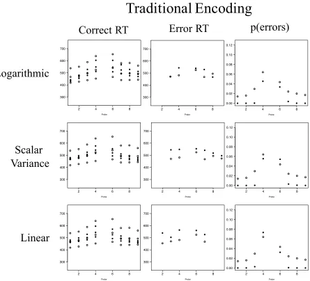
We then ran six random walk models: three theories of quantity distributions for each of the two simulation models (Traditional and Encoding Errors). We fit each simulation,
simultaneously, to the 25th, 50th, and 75th percentile score for each probe for the correct RTs, the 50th percentile score for the error RTs, and the proportion of errors.
To optimize the fit of the parameters, we implemented a semi-random grid search method. In preliminary runs of the simulation, we discovered that standard optimization
procedures were extremely sensitive to the start point of the parameter search. Because we could not assume we had valid start points, we explored new methods for optimization. Systematic grid-search methods are exponentially inefficient as the number of parameters increases. It has been demonstrated that random search methods are far more efficient and produce equally good model fits (Bergstra, & Bengio, 2012). We therefore programmed a semi-random grid-search optimization method to identify initial start points to be used with existing optimization procedures. However, after implementing our procedure, we discovered it produced superior parameter estimates to existing procedures. Furthermore, in using our proceduresÕ best-fit parameter estimates as start points for more established optimization procedures, we discovered that there were no further improvements in the fit statistics. Therefore, we used our optimization procedure exclusively. Our optimization procedure is as follows.
probe using the parameter values chosen. In first calibration, the optimization program ran 50 simulations. From these 50 simulations, the 15 best were identified. For each parameter, the high and low parameter values from this set of 15 were identified and used as the new high and low boundaries. The procedure was repeated, with the number of simulations runs increasing by 50% before each re-calibration, until the model fit did not increase three calibrations in a row. At this point, a fine-grained procedure was implemented, whereby the high and low boundaries were set at either 5% above and below the best-fit parameter or remained at the last value, whichever was smaller. Furthermore, the number of trials simulated per run was increased to 5000. The procedure was repeated, with the number of simulations increasing by 50% with each re-calibration, until the model fit did not increase three calibrations in a row. At this point, the best-fit parameters were identified as the final parameters, and a final simulation was run with 10,000 trials per probe. We note that the quantities chosen in the simulation (e.g., 50 simulations per calibration, 15 best runs, 400 trials per run, etc.), were those used to optimize the
performance of the system (i.e., its efficiency and ability to converge on the best fit parameter) in preliminary testing of the optimization program.
simulations, we did not want to disqualify them. We therefore standardized all BIC measures by dividing the BIC by the number of points the model fit (termed BICz). We note here that the
Error Encoding model has one extra parameter than the Traditional model. The Error Encoding model adds the k parameter, which identifies the probability that the environment will be
sampled. As the proportion of encoding errors is pre-specified in Table 1, error encoding in itself does not add a free parameter. We also calculated the chi square using a method similar to Ratcliff and Tuerlinckx (2002; see also Ratcliff & Childers, 2015). Because chi square,
calculated in this way, is sensitive to the number of samples (we ran 10,000 samples per probe) and the number of conditions (we summed over 8 probes), the absolute value of the chi square is not meaningful. Nevertheless, the relative values of the chi square between models provides information about the relative fits of the models.
Because RT and error proportion were on different scales, we calculated r2 separately for each. For some of the models, the simulations could not simultaneously fit the RT and error proportion. This resulted in an error proportion r2 that was less than 0. When this was the case, we set the error proportion r2 = 0. We used the average of the two r2s as our fit statistic.
Because, r2 is the measure of the percent of variance in the data that is accounted for by the model, it does not provide a statistical advantage for fitting fewer points. However, r2 does not penalize for added parameters.
Statistically, r2should be negatively correlated with both the BICz and the chi square.
We found significant negative correlations between the BICz and r2, r(5)= -.98, p<.05, and the
chi square and r2, r(5)= -.99, p<.05, fit statistics of our six models. There was also a positive correlation between the BICz and chi square, r(5)= .97, p<.05. Because all three fit statistics were
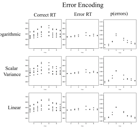
remainder of the analysis4. Figure 4 shows a plot of r2 for the simulations of the 6 models we ran: 3 quantity representations (Linear Theory, Logarithmic Theory, and Scalar Variance Theory, respectively) X 2 random walk models (Traditional Encoding and Error Encoding). Table 3 presents the best-fit parameter values for each model. Figure 5 shows plots of the behavioral data and the data simulated with the Traditional Encoding model for the three quantity representations. Figure 6 shows plots of the behavioral data and the data simulated with the Encoding Errors model for the three quantity representations.
The simulations clearly show that the Encoding Errors model, regardless of
representation, fits the data better than the Traditional Encoding model. The r2 for the Encoding Errors models ranged from .73-.88, whereas the r2 for the Traditional Encoding models ranged from .14-.27. The Traditional Encoding model has the most difficulty fitting the error RT data and the proportion of errors. In fact, not one of the Traditional encoding models was able to simultaneously fit all the RT data and match the behavioral error proportions. In contrast, when encoding errors were introduced with the Error Encoding models, all three representations produced superior fits. It is of some considerable importance to note that it is a trivial matter for the Traditional Encoding model to fit the mean correct RT alone using any of the three quantity representation theories. It is only when the model is required to fit the correct and error RT as well as the proportion of errors that it fails.
The second clear finding is that the Linear representation, regardless of model, fit the data better than the Logarithmic or Scalar Variance models. Although the Scalar Variance
and Logarithmic Theory representations (Cantlon et al., 2009; Dehaene et al., 2008). This finding demonstrates that the size effect is not necessarily a function of the compression in the
psychological representation of quantity (as is commonly believed).
All models converged on an angled decision threshold. The angled threshold reduces the amount of evidence required for a response as time increases. The angle has the effect of
reducing the skew of the data as well as influencing the probability of an error. The finding that all models converged on an angled threshold is interesting because, in instances where one is pressed for time, it has been traditional to assume the thresholds move closer to the Ò0Ó evidence line. Allowing the threshold to be angled provides another source for time pressure to influence the data. Specifically, the angle may steepen. As Zhang et al. (2014) intimated, there are many interesting and unexplored questions that arise when time-varying boundaries are incorporated into sequential sampling models of human decision-making.
Discussion
The results of the simulations are strikingly clear: the Encoding Errors models produced superior fits to the behavioral data from the relative quantity task (Figures 5 and 6) when compared against the Traditional Encoding models. The Encoding Errors models are based on the key assumption that encoding processes are prone to error and that this error can be
striking (see Figure 5) considering the very strict constraints imposed on the modeling, namely, (i) the distribution of the human correct and error data were fit simultaneously; (ii) only the most extreme scores were removed from the data prior to the modeling; and (iii) the encoding
confusion probabilities were set a priori by the formula developed by Cohen (2009). In addition to assessing the validity of the Encoding Error model vs. the Traditional Encoding model, we compared the relative abilities of the three primary theories of quantity representation (see Figure 1B) to fit the behavioral data in the relative quantity task. We
examined each of these quantity representations in terms of error-less (Traditional Encoding) and error-prone encoding (Encoding Errors) mechanisms. When considered at this level of detail, the data clearly show that the Linear version of the Encoding Errors model provides the best fit to the data. Indeed, the finding that the Linear Theory models performed best stands in stark contrast to how the extant models are currently perceived (Cantlon et al., 2009; Dehaene et al., 2008). In the extant literature, key arguments have focused on the relative strengths and weaknesses of the Logarithmic Theory and Scalar Variance Theory on the basis of the false assumption that the Linear Theory does not adequately account for the size effect. It should be noted that, although the Logarithmic Theory and Scalar Variance Theory have popular appeal among researchers, most computer simulations of numerical cognition assume the Linear Theory representation (e.g., Link, 1990). The attraction of the Logarithmic Theory and Scalar Variance Theory accounts likely results, in part, from their intuitive ability to predict the correct RT data in the relative quantity task. However, as our current simulations show, none of these models can accommodate task performance when this is defined comprehensively, that is, it
simulations showing fits only to average correct RT in the task conditions (e.g., Verguts, et al., 2005). We conclude therefore that it is no longer sensible to attempt to adjudicate between the models solely in terms of fits to average correct RTs.
The Role of Perceptual Encoding
Our simulation shows the importance of encoding processes to observersÕ behavior in the relative quantity task. Specifically, the Linear Encoding Errors model assumes that (i) the numerical symbol that is physically present is continuously sampled, (ii) each sample has a probability of mis-encoding the symbol, and (iii) a perceived quantity is derived from each sample that contributes to the observerÕs cumulative understanding of the quantity associated with the numerical symbol. As a result, the encoding process directly influences the observerÕs intuitive understanding of the quantity associated with each symbol. For example, assume an observer is presented a Ò9.Ó On Trial A, the observer samples the 9 as a Ò9Ó most often, but occasionally as a Ò4.Ó In contrast, on Trial B, the observer samples the 9 as a Ò9Ó most often, but occasionally as a Ò7.Ó In this situation, the observerÕs intuitive sense of quantity associated with the Ò9Ó would be lower on Trial A than on Trial B because of the influence of the error-prone encoding process.
such that the likelihood of re-sampling decreases as the number of steps taken in the random walk increases. When memory updating does not take place on a given step in the walk, the memory representation of the input digit is taken to be the most frequently sampled value. In this way, the system will converge on the correct encoding over time. That is, because the correct digit is the most likely digit to be encoded, it will be the most frequently sampled value over time. Thus, an Encoding Errors account as we described may be an optimal system: it will be efficient because encoding and accessing meaning occur simultaneously, and any errors of mis-perception are corrected over time. From this theoretical perspective, encoding, storage, and retention are intimately connected in ways that have not previously been examined. Indeed, at one level, the current work provides an existence proof that the sorts of ideas regarding error-prone perceptual sampling hold much potential. Indeed, it seems important in the future to examine the relative explanatory power of the exponential decay function of equation 7 when compared against other plausible alternatives.
Given the novelty of Encoding Errors model it is only possible to speculate about the possible consequences for general theories of perception. The Encoding Errors model accords with the fact that vision takes places within a constantly changing environment. As a
consequence, perceptual impressions of the world are in a constant state of flux. Because
ambiguous visual signals (Ernst & BŸlthoff, 2004). Repeatedly sampling the input averages out random noise, thus helping reduce perceptual ambiguities. There is every reason to suppose that the current notions of continuous encoding generalize to other aspects of cognition and
perception (Norris, 2006; see also Norris & Kinoshita, 2008).
We suspect that the k parameter is not fixed and may be under some cognitive control. That is, when focal attention is applied and the task requires conscious identification of the stimulus, the k parameter may tend towards 0 (but likely not reach 0). However, when scanning the visual field quickly, where time is decreased and the amount of visual information is
increased, the k parameter may tend toward 1. Under these circumstances it is assumed that there is no memory for the encoded identity of the stimulus. However, there is memory for the semantic meaning of the stimulus. In this way, the visual system retains the gist of the visual field without storing potentially unnecessary details. Such a system is efficient because the environment contains the relevant information, which can be referred back to via a saccade, which is not also duplicated as a memory representation. Such a system may provide a mechanism for explaining change blindness (Simons & Ambinder, 2005).
perceived quantities generated from the Encoding Errors model produce a negatively decelerating function similar to the log.
The negatively decelerating function in Figure 7 describing the intuitive sense of amount denoted by numerical symbols is of central importance to linking the present simulation to previous research. Specifically, much of the previous research has concluded that the quantity associated with numerical symbols was represented on a logarithmic scale because of the size effect. Our simulation revealed that the Logarithmic Theory representation does not actually fit the behavioral data very well. Rather, we concluded that the current evidence favors the Linear Theory and this falsifies the intuition that the model cannot accommodate the basic size effect. The important question therefore is, ÔHow does the Linear Theory accommodate the size effect?Õ The negatively decelerating function in Figure 7 suggests that the size effect manifests primarily from encoding processes, rather than the underlying quantity representation. This contention is supported by the fact that none of the three primary quantity representations fit the size effect well with the Traditional Encoding account, despite the fact that both the Logarithmic and Scalar Variance accounts have negatively decelerating functions. It is only after encoding errors are added that the size effect is fit adequately by all of the quantity representation variations.
Further insights and implications
One notable aspect of the random walk models examined here concerns the nature of the response thresholds. As in all previous incarnations of random walk models, the walk takes place in a 2-D Euclidian plane. The start position is a point on the y-axis and the walk proceeds until it reaches one of two decision boundaries. In the majority of previous random walk models the boundaries are fixed and are perpendicular to the y-axis. In the current modeling we have retained the idea that the y intercepts of the boundaries are fixed but have defined their angle of intersection (b) with the y-axis as a free parameter (see Figure 3A). We have provided another concrete example of where the incorporation of time-varying boundaries in sequential sampling models enhances their explanatory power (cf. Zhang et al., 2014). A simplifying assumption has been that the angle of incidence for both smaller and larger decision boundaries is constrained to be the same but it would be desirable that future work examines the consequences of relaxing this symmetry assumption. Nonetheless a key feature of the current account is that the angle of incidence of the response boundaries is not fixed.
random walk models and, in agreement with Zhang et al. (2014), we suggest that this could be examined more generally when using such models in future.
z - the start point of the walk
A central feature of our simulations was the fact that we modeled correct and error RT as well as the proportion of errors for every probe simultaneously. Although other researchers have suggested that simulating the error proportions obtained from the behavioral data is trivial
(Verguts et al., 2005), our simulations suggest that they are, in fact, one of the key characteristics of the data that can be used to distinguish the different models. In particular, although the
numerical distance effect is clearly present in the error proportions, there is a key inconsistency with this pattern and the pattern predicted by compressed quantity representations such as the Logarithmic and Scalar Variance accounts. The compressed quantity representations predict that the errors produced in response to the larger numbers (when compared to a standard of 5) will be greater than their symmetrical counterparts. So, for example, the errors produced in response to a Ò6Ó should be greater than those produced in response to a Ò4.Ó We see in the behavioral data, however, that this is not the case for the Ò4Ó and the Ò6.Ó This is again a reason to question the explanatory adequacy of the Logarithmic and Scalar Variances models.
Our simulations account for this ÒbackwardsÓ data by shifting the start point (the z
parameter) towards the ÒsmallerÓ threshold: z is negative in all cases (see Table 3). Indeed, for the Error Encoding models (i.e., the only models that fit well), the larger the compression of the original quantity representation on which the model was simulated, the larger the shift of the start point. Because the Linear Theory is not compressed, it did not require the simulations to
quantity representations produced patterns in which the Ò4Ó had fewer errors than the Ò6.Ó Here again therefore is an example of the utility of having an explicit computational model. In this case it has provided an effective tool that can be used to test intuitions about both data and theory.
Of Models and Modeling
The present work emphasizes the contribution that models and modeling can make to theory development and assessment. We have shown how a relatively simple task translates into a fairly complicated set of cognitive processes. However, when these processes are stated precisely, then different theories can be weighed against one another via the relative fits they provide to the behavioral data. Although we have focused on understanding performance in the relative magnitude task, we feel that the implications of the work go further than this and do speak to issues that have arisen with other numerical tasks. Perhaps the most prominent amongst these is the cross modal matching paradigm in the form of the number line task (see e.g.,
Berteletti, Lucangeli, Piazza, Dehaene, & Zorzi, 2010; Booth & Siegler, 2006; Cohen & Blanc-Goldhammer, 2011; Dehaene, Isard, Spelke, & Pica, 2008; Geary, Hoard, Nugent & Bryd-Craven, 2008; Siegler & Booth, 2004). The number line task requires the encoding and
processing of both digits and lines, as well as relatively complex cross modal matching. These complications are often glossed over in the literature and the processes involved with completing the task are rarely modeled.
not attempted to compare random walk models with neural network counterparts: this would be a major and different undertaking altogether. However, we do note that the neural network models of numerical cognition appear wanting when assessed against the hard constraints discussed here.
For instance, the network models described by Verguts et al. (2005) do not address the full complement of the kinds of behavioral data considered here, namely, correct and error RT distributions, and error proportions. Verguts et al (2005) primarily focused on their modelÕs ability to fit mean correct RT in various number tasks and respectable fits are reported via this level of analysis. Although they offer a promissory note about an Òadditional stochastic
component,Ó and claim that the error data do not Òpose a significant challenge to the modelÓ (p. 78), it remains to be seen whether their model can account for these data. Indeed, our data reveal that modeling mean RTs proves no challenge to any of the three key theories of number
representation. It is only when the full complement of data is considered is it possible to
discriminate between the explanatory power of the different models. On these grounds, it will be interesting to see how neural network models fair when the full complement of data is taken into account.
Prospects for future work
Provision of the current computer simulations is an important step in understanding the numerical cognition system. Nevertheless, this work is not without some limitations. First, we identified the Error Encoding models as proving superior to the Traditional Encoding models, yet we have to explore fully and test the Error Encoding modelÕs predictions. For example, the Error Encoding model appears to predict that adding visual noise to the presented numerals will
Furthermore, limiting encoding time should have a predictable effect. These, and other,
predictions require testing. In addition, it is unclear how the Error Encoding model will account for the SNARC effect (Dehaene, Bossini & Giraux, 1993). In the current work, we
counterbalanced response button, so the SNARC effect should not influence the results in a meaningful way. Most models of numerical cognition adopt a post hoc explanation for the SNARC effect, and we will consider possible explanations for the effect in future versions.
A second limitation of the current model is that it was run as a computer simulation of a discrete random walk model and this is distinctive against a background of the other work that has considered random walk models based on diffusion processes (e.g., Smith & Mewhort, 1998). Clearly future work might be directed to extending the modeling to examine the
consequences of adopting a continuous rather than discrete random walk. We adopted the present methods because the different quantity representations (logarithmic distributions, unequal
variances) and the Encoding Errors model (simultaneous encoding and comparisons) pose considerable mathematical challenges to the derivation of an analytic solution. Addressing these challenges could form the basis of a primarily mathematical rather than psychological exercise and is simply beyond the scope of this present paper.
2009). We assume further progress will be made once details about the encoding of more complex numbers are uncovered.
Some previous work with double-digit integers (Cohen, 2010) has revealed that factors associated with encoding do play a determining role in quantity judgments. In one of the experiments reported by Cohen (2010) speeded quantitative judgments were made in cases where participants judged whether a probe (in the range 1 Ð 99) was greater/ less than 55. Although effects of numeral distance were present in the data, best fits to the data depended on including factors concerning physical similarity of the decade of the double digits.
Evidence from the other experiments concerning decimals (Cohen, 2010) however was quite different and showed very strong effects due to physical similarity. Indeed, in one experiment no effects of numerical distance on task performance were observed when physical similarity was taken into account. In these cases, the decimals (.01 - .99) were judged relative to the standard .55. In the latter experiment participants were forced to attend to the position of the decimal point by varying the rounding of the numbers across trials. When all decimals were presented to the same level of precision participants may simply have ignored the decimal point and treated the numbers as being integers. Clearly, therefore, when attention is focused more broadly on a range of number formats other than single digits more complex accounts of performance are needed. We accept that these will demand a proper consideration of encoding processes.
Conclusions
quantity from behavioral data, it is important to consider very carefully the influences of encoding, decision, and response execution as well as other, more salient task related processes such as comparison, on the participantsÕ responses. We have instantiated the primary models of numerical cognition in computational models of the relative quantity task. Our data reveal that (i) encoding processes influence performance in non-negligible ways, (ii) quantities are
represented as perceptual distributions that are equally spaced and have equal variance, (iii) the perceptual system repeatedly samples the stimulus in an error-prone fashion, and, (iv) the recovery of number meaning proceeds in parallel with, and is continuously influenced by, stimulus encoding. Together, these findings represent a new and comprehensive understanding of the perceptual and cognitive mechanisms that underpin human number comparison. We feel that consideration of these ideas gives rise to more wide-reaching implications for thinking about how the human perceptual system operates in general.
References
Ashby, F. G. (2000). A stochastic version of general recognition theory. Journal of Mathematical Psychology, 44, 310-329. http://dx.doi.org/10.1006/JMPS.1998.1249
Ashby, F. G., & Maddox, W. T. (1994). A response time theory of separability and integrality in speeded classification. Journal of Mathematical Psychology, 38, 423-466.
http://dx.doi.org/10.1006/jmps.1994.1032
Balakrishan, J. D., & Ratcliff, R. (1996). Testing models of decision making under confidence ratings in classification. Journal of Experimental Psychology: Human Perception and Performance, 22, 615-633. http://dx.doi.org/10.1037/0096-1523.22.3.615
Banks, W. P., Fum, M., & Kayra-Stuart, F. (1976). Semantic congruity effects in comparative judgments of magnitudes of digits. Journal of Experimental Psychology: Human Perception and Performance, 2, 435-447. http://dx.doi.org/10.1037/0096-1523.2.3.435
Bergstra, J., & Bengio, Y. (2012). Random search for hyper-parameter optimization. Journal of Machine Learning Research, 13, 281-305.
Berteletti, I., Lucangeli, D., Piazza, M., Dehaene, S., & Zorzi, M. (2010). Numerical estimation in preschoolers. Developmental Psychology, 46, 545-551.
http://dx.doi.org/10.1037/a0017887
Booth, J. L., & Siegler, R. S. (2006). Developmental and individual differences in pure number estimation. Developmental Psychology, 41, 189-201.
Buckley, P. B., & Gillman, C. B. (1974). Comparisons of digits and dot patterns. Journal of Experimental Psychology, 103, 1131-1136. http://dx.doi.org/10.1037/h0037361
Cantlon, J. F., Cordes, S., Libertus, M. E., & Brannon, E. M. (2009). Comment on ÒLog or Linear? Distinct Intuitions of the Number Scale in Western and Amazonian Indigene CulturesÓ. Science, 323. http://dx.doi.org/10.1126/science.1164773
Cantlon, J. F., Platt, M. L., & Brannon, E. M. (2008). Beyond the number domain. Trends in Cognitive Science, 13, 83-91. http://dx.doi.org/10.1016/j.tics.2008.11.007
Church, R. M., Meck, W. H., & Gibbon, J. (1983). Application of scalar timing theory to individual trials. Journal of Experimental Psychology: Animal Behavior Processes, 9, 135-155. http://dx.doi.org/10.1037/0097-7403.20.2.135
Cohen, D. J. (2009). Integers do not automatically activate their quantity representation.
Psychonomic Bulletin & Review, 16, 332-336.
http://dx.doi.org/10.3758/PBR.16.2.332
Cohen, D. J. (2010). Evidence for Direct Retrieval of Relative Quantity Information in a
Quantity Judgment Task: Decimals, Integers, and the Role of Physical Similarity. Journal of Experimental Psychology: Learning, Memory and Cognition, 36, 1389-1398.
http://dx.doi.org/10.1037/a0020212
Cohen, D. J., & Blanc-Goldhammer, D. (2011). Numerical bias in bounded and unbounded number line tasks. Psychonomic Bulletin and Review, 18, 331-338.
http://dx.doi.org/10.3758/s13423-011-0059-z
Curtis, D. W., Paulos, M. A., & Rule, S. J. (1973). Relation between disjunctive reaction time and stimulus difference. Journal of Experimental Psychology, 99, 161-173.
http://dx.doi.org/10.1037/h0034637
Dehaene, S. (1992). Varieties of numerical abilities. Cognition, 44, 1-42.
http://dx.doi.org/10.1016/0010-0277(92)90049-N
Dehaene, S. (2003). The neural basis of the WeberÐFechner law: a logarithmic mental number line. Trends in Cognitive Science, 7, 145-147. http://dx.doi.org/10.1016/S1364-6613(03)00055-X
Dehaene, S., & Akhavein, R. (1995). Attention, automaticity, and levels of representation in number processing. Journal of Experimental Psychology: Learning, Memory, and Cognition, 21, 314-326. http://dx.doi.org/10.1037/0278-7393.21.2.314
Dehaene, S., Bossini, S., & Giraux, P. (1993). The mental representation of parity and number magnitude. Journal of Experimental Psychology: General, 122, 371-396.
http://dx.doi.org/10.1037/0278-7393.21.2.314
Dehaene, S., Dupoux, E., & Mehler, J. (1990). Is numerical comparison digital? Analogical and symbolic effects in two-digit number comparison. Journal of Experimental Psychology: Human Perception and Performance, 16, 626-641. http://dx.doi.org/10.1037/0096-1523.16.3.626
Dehaene, S., Isard, V., Spelke, E., & Pica, P. (2008). Log or linear? Distinct intuitions of the number scale in Western and Amazonian indigene cultures. Science, 320, 1217-1220.
Dehaene, S., Naccache, L., Le Clec, H. G., Koechlin, E., Mueller, M., Dehaene-Lambertz, G., et al. (1998). Imaging unconscious semantic priming. Nature, 395, 597-600.
http://dx.doi.org/10.1038/26967
Ernst, M. O., & BŸlthoff, H. H. (2004). Merging the senses into a robust percept. Trends in Cognitive Science, 8, 162-169. http://dx.doi.org/10.1016/j.tics.2004.02.002
Feigenson, F., Dehaene, S., & Spelke, E. (2004). Core systems of number. Trends in Cognitive Science, 8, 307-314. http://dx.doi.org/10.1016/j.tics.2004.05.002
Gallistel, C. R., & Gelman, R. (1992). Preverbal and verbal counting and computation.
Cognition, 43-74. http://dx.doi.org/10.1016/0010-0277(92)90050-R
Ganor-Stern, D., & Tzelgov, J. (2008). Across-notation automatic numerical processing. Journal of Experimental Psychology: Learning, Memory, and Cognition, 34, 430-437.
http://dx.doi.org/10.1037/0278-7393.34.2.430
Garc’a-Orza, J., Perea, M., Mallouh, R. A., & Carreiras, M. (2012). Physical similarity (and not quantity representation) drives perceptual comparison of numbers: Evidence from two Indian notations. Psychonomic Bulletin & Review, 19, 294-300.
http://dx.doi.org/10.3758/s13423-011-0212-8
Geary, D. (1994). Children's mathematical development: Research and practical applications. Washington, DC: American Psychological Association.