Rochester Institute of Technology
RIT Scholar Works
Theses Thesis/Dissertation Collections
2006
Acoustic classification using independent
component analysis
James Brock
Follow this and additional works at:http://scholarworks.rit.edu/theses
This Thesis is brought to you for free and open access by the Thesis/Dissertation Collections at RIT Scholar Works. It has been accepted for inclusion in Theses by an authorized administrator of RIT Scholar Works. For more information, please [email protected].
Recommended Citation
Acoustic Classification Using
Independent Component Analysis
by
James L. Brock
A Thesis Submitted in Fulfillment of the Requirements for the Degree of Master of Science in Computer Science
Supervised by
Director, Laboratory of Intelligent Systems Dr. Roger Gaborski Department of Computer Science
Golisano College of Computing and Information Sciences Rochester Institute of Technology
Rochester, New York May 2006
Approved By:
Dr. Roger Gaborski
Director, Laboratory of Intelligent Systems Primary Advisor
Carl Reynolds Visiting Professor
Thesis Release Permission Form
Rochester Institute of Technology
Department of Computer Science
Title: Acoustic Classification Using Independent Component Analysis
I, James L. Brock, hereby grant permission to the Wallace Memorial Library to
repro-duce my thesis in whole or part.
James L. Brock
Acknowledgments
I would first like to thank my thesis advisory committee, Dr. Roger Gaborski, Dr. Carl
Reynolds, and Dr. Peter Anderson. I would also like to thank everyone that helped and
supported me along the way to completing this work. Last, but not least I would like to
Abstract
This thesis research investigates and demonstrates the feasibility of performing
computa-tionally efficient, high-dimensional acoustic classification using Mel-frequency cepstral
co-efficients and independent component analysis for temporal feature extraction. A process
was developed to calculate Mel-frequency cepstral coefficients from samples of acoustic
data grouped by either musical genre or spoken world language. Then independent
compo-nent analysis was employed to extract the higher level temporal features of the coefficients
in each class. These sets of unique independent features represent themes, or patterns, over
time that are the underlying signals in that class of acoustic data. The results obtained from
this process clearly show that the uniqueness of the independent components for each class
Contents
Acknowledgments . . . iii
Abstract . . . iv
1 Introduction. . . 1
1.1 Motivation . . . 1
1.2 Auditory Cognition . . . 2
1.3 Thesis Outline . . . 3
2 Background . . . 5
2.1 Biological Inspiration . . . 5
2.2 Mel-Frequency Cepstral Coefficients . . . 8
2.3 Principal Component Analysis . . . 11
2.3.1 Theoretical Background . . . 11
2.3.2 Process . . . 14
2.3.3 Examples . . . 15
2.4 Independent Component Analysis . . . 17
2.4.1 Introduction to ICA . . . 17
2.4.2 Theoretical Background . . . 19
2.4.3 Independence . . . 22
2.4.4 Measuring Independence . . . 23
2.4.5 ICA and Projection Pursuit . . . 27
2.4.6 Preprocessing . . . 28
2.4.7 FastICA Algorithm . . . 29
2.4.8 Temporal vs. Spatial ICA . . . 31
2.4.9 Use in Cognitive Modeling . . . 32
3 Cognitive Model . . . 36
3.2 Process Development . . . 38
3.2.1 Preprocessing . . . 38
3.2.2 ICA for Feature Extraction . . . 39
4 Process Implementation . . . 42
4.1 Data Set . . . 42
4.1.1 Test Tones . . . 43
4.1.2 Music Genres . . . 44
4.1.3 World Languages . . . 44
4.2 Preprocessing . . . 45
4.2.1 Random Sampling . . . 45
4.2.2 Calculating MFCC’s . . . 46
4.3 Independent Feature Extraction . . . 48
5 Results Analysis. . . 51
5.1 Initial Experiments (Tones) . . . 51
5.2 Musical Genres . . . 53
5.2.1 Principle Component Separation . . . 54
5.2.2 Independent Component Separation . . . 56
5.3 World Language . . . 58
5.3.1 Principle Component Separation . . . 58
5.3.2 Independent Component Separation . . . 59
6 Conclusions . . . 69
7 Future Work . . . 70
Bibliography . . . 71
A Source Code (MATLAB) . . . 74
A.1 README.m . . . 75
A.2 main.m . . . 76
A.3 init.m . . . 79
A.4 readNextFile.m . . . 79
A.5 sparsMFCC.m . . . 80
A.6 plotComps.m . . . 81
List of Figures
2.1 Auditory Cortex Model[2] . . . 6
2.2 Human cochlea, which reacts in different areas to different frequencies of sound [2] . . . 8
2.3 MFCC process(left)[5] and Mel-scale filter bank(right)[22] . . . 9
2.4 Band-passed frequency response of a jazz song . . . 10
2.5 Raw data(left) and normalized data with eigenvectors superimposed(right) . 14 2.6 Example eigenfaces . . . 16
2.7 Linear combinations of eigenfaces reconstruct original images . . . 16
2.8 Cocktail party problem using ICA[6] . . . 18
2.9 Example source signals[22] . . . 21
2.10 Example mixed signals[22] . . . 21
2.11 Sources extracted using ICA[22] . . . 21
2.12 Speech joint PDF (left), Gaussian joint PDF (right) . . . 23
2.13 Graph of entropy relative to probability of a coin toss[1](left), plot of 3 variables with maximum entropy (right) . . . 25
2.14 Grouping of underbrush images(left) and horizons(right) [17] . . . 34
3.1 Music preprocessing results from [16] (left), and recreated results (right) . . 37
3.2 Acoustic preprocessing of one piece acoustic data . . . 39
3.3 Training process for a single MFCC for a single group . . . 40
3.4 Points of comparison for classes of acoustic data . . . 41
4.1 Example test tones, burst (left) and ramp (right) . . . 43
4.2 Grouping of audio samples . . . 46
4.3 Grouping MFCC’s for each signal and all groups into feature matrices . . . 47
4.4 Grouping of independent components into points of comparison for the groups of acoustic data . . . 49
5.2 Burst sawtooth wave plot of principal components (left) and histogram of principal component 1 . . . 54
5.3 Frequency ramp plot of principal components (left) and principal
compo-nent 1 over time . . . 55 5.4 Principle components for 6 different MFCC’s, demonstrating statistical
in-dependence and separation (2D) . . . 61 5.5 Principle components for 4 different MFCC’s, demonstrating statistical
in-dependence and separation (3D) . . . 62
5.6 Independent temporal features for 4 different MFCC’s (2D) . . . 63
5.7 Independent temporal features for 4 different MFCC’s (3D) . . . 64
5.8 Principle components for 4 different MFCC’s, demonstrating statistical in-dependence and separation (2D) . . . 65 5.9 Principle components for 4 different MFCC’s, demonstrating statistical
Chapter 1
Introduction
1.1
Motivation
Advancements in networking technology and globalization have spawned a quickly
ex-panding digital media market. This market has given all classes of individual access to
on-demand videos, music, movies, etc. and created the growing problem of how to
iden-tify, classify, organize, and manage this media. Traditionally, this problem has been
ad-dressed with humans classifying the media and constructing meta data stored with each
file to identify its characteristics, because content recognition is a seemingly trivial task for
the average person. It has become quite obvious in recent years that the amount of digital
media present in the world is far too great to use this method to identify the characteristics
of a file’s content in an efficient manner.
In the music world specifically this problem has come to the forefront with the inception
of online stores for digital music (iTunes, Yahoo! Music, RealMusic, etc.) and streaming
audio services such as Pandora (based off of the Music Genome Project), Yahoo! Launch,
and internet radio. These services use advanced queries of the user-specified meta data to
search through their databases and cater to the listener’s preferences. However, not only is
musical preference extremely unique, but the classification of music is a matter of personal
opinion as well, since there is no standard for musical genres and sub-genres. A song one
person considers to beclassic rock may beoldiesto another and stillacid rockto another,
intelligently classify digital music, and other media, based on some loose criteria.
This problem can easily be extended to all kinds of acoustic information and databases.
Records of speech, animal noises, and other sounds used in scientific research and
surveil-lance are difficult to maintain without some working knowledge of the content of each
piece of data. A general process for acoustic classification would enable the majority of
this data to be automatically classified and produce meta data that would ease the cost of
time and computing resources necessary to do so through traditional means. The feasibility
of such a process is the primary motivation for this thesis research into a successful means
by which all acoustic information can be automatically classified, beginning with music
and extending it to world languages.
1.2
Auditory Cognition
The human auditory system has been the subject of research for quite some time and
re-sulted in information concerning how to represent and mimic its basic behavior. It’s been a
consistent problem, however, to model the higher-level functionality and acoustic
interpre-tation of human hearing and cognition. Though there is still a great deal of debate on which
is best, most current models break down human hearing into hierarchal, functional layers
much like the modeling of the visual cortex. Since much more work has been done in the
field of computer vision and modeling the visual cortex, a great deal of the research done on
the auditory cortex is based off of successful algorithms and concepts from the area of
com-puter vision. One of these areas of research is the human ability to distinguish accurately
between different types of sounds almost instantly. Human beings are able to distinguish
the sources, characteristics, and general location of most sounds easily allowing them to
classify them as significant or group them together. It is a current area of research
devel-oping algorithms that achieve this level of cognitive performance in response to acoustic
This thesis will discuss and develop an approach to modeling the higher-level
cogni-tion of the human auditory system in a way that makes automatic classificacogni-tion of acoustic
information using independent component analysis quit feasible. An audio processing
al-gorithm will be constructed using Mel-frequency cepstral coefficients, principal component
analysis, and independent component analysis to separate acoustic information in the form
of music and foreign languages.
1.3
Thesis Outline
This thesis will begin with a background explanation of the major concepts and subject
matter used in this work, including Mel-frequency cepstral coefficient, principal
compo-nent analysis, and independent compocompo-nent analysis. Material and results from work done
within the domain of signal processing, source separation, and acoustic understanding will
be presented in support of this research. This chapter will also explain the biological
in-spiration for using the aforementioned techniques in modeling the human auditory system
and its cognitive properties. The third chapter will explain the process of developing a
novel process for acoustic information separation based on previous work and techniques
used in this area. Model diagrams will demonstrate the flow and processes used to extract
significant features, separate the feature set using independent component analysis, and
then demonstrate the independence of groups of acoustic information. The process will
also be explained conceptually to give a general overview of how this is able to support
simple high-level acoustic classification while taking particular time to highlight the most
significant parts of the algorithm.
Chapter four of this thesis will delve deeply into the technical aspects of the developed
process, siting specific values, parameters, algorithms, and audio signal processing steps
taken to achieve optimal results. Each step of the process will be explained in the context
of the conceptual description and each modification and technical choice explained fully,
along the way. This chapter will also explain how the process was organized and give
details about the acoustic information and databases used for this research.
The fifth chapter will explain the results achieved and evaluate the algorithm’s
perfor-mance, making note of where, how, and why the process either succeeded or gave marginal
results. The results will be evaluated and explained in order to correlate unexpected
perfor-mance with the particular part of the process that is the source of any discrepancies. Finally,
the sixth chapter will give final conclusions about the thesis work and results achieved in a
more general context, also suggesting areas for future research to be done in this problem
Chapter 2
Background
2.1
Biological Inspiration
The human auditory cortex is a complex cognitive system, able to make extremely
selec-tive and complex decisions in an instant. This performance has long been desired in the
field of intelligent systems and signal processing. Research is always being done to try to
model, mimic, and further understand this system. There are many models for how
differ-ent researchers believe the auditory cortex functions at the neurological level. One common
model is shown in figure 2.1. Where the objects labelled as PFC, PP, and PB are the
pre-frontal connections, posterior parietal cortex, and parabelt cortex respectively. These are
the biological parts of the brain that handle the highest levels of auditory interpretation and
interfacing with the rest of the brain [23]. The exact function and mechanics are beyond
the scope of this work. The other regions depicted in the diagram, however, are the exact
part of the auditory cortex that this approach to acoustic classification is trying to model
and will be explained further.
The primary purpose of this diagram is to map the ”Where” and ”What” paths of the
au-ditory cortex, with ”Where” shown in Red and ”What” shown in Green [23]. The ”Where”
path is the path through the brain audio signals take to determine the spatial information
of the sound. The ”Where” path is the same thing, but for identifying the type of sound.
The set of rectangular areas labeledCortex andThalamuson the right side of the diagram
Figure 2.1: Auditory Cortex Model[2]
Those regions are organized into three subsections, the caudal belt (labeled belt in figure
2.1), the core, and the thalamus [23]. The thalamus is the first step in higher-level auditory
cognition, as acoustic information from the ear enters the auditory cortex via the medial
geniculate nucleus (MGN, sometimes combined with the cochlear nuclei) within it,
mak-ing it the primary auditory relay nucleus. The MGN is broken up into ventral and dorsal
parts, with the dorsal part focused on spatial information, and the ventral part focused on
temporal and frequency information.
As shown in figure 2.1, audio data flows from the two parts of the MGN to the two
par-allel spatial cortex regions (CL and CM) and identifying cortex regions (R and AL). The
arrows depicting the flow of information have been biologically proven by tracing
connec-tions between the regions in various human and non-human primates [23]. There is also, a
couple unifying regions of the cortex (ML and A1) that respond to both types of audio data,
but perform some distinction to pass appropriate information onto the other regions. None
spatial information, and ML and A1 both respond well to all kinds of acoustic information.
However, the important aspect of the auditory cortex’s functionality to take away from this
is that both spatial information and other information, such as temporal features, frequency
changes, and amplitude changes, are processed in parallel and the human brain does make
a distinction between them [23]. The purpose of the work in this thesis is to model the
higher-level cognition of the ”What” path, using identifying temporal themes with regards
to frequency to show that somewhat intelligent distinctions can be made computationally.
For relevant audio processing applications, researchers are continually trying to model
this higher-level operation quantitatively. Recent work has determined that independent
component analysis (ICA) is a sufficient method for modeling some of the higher-level
interpretation of sensory information in humans [16],[17]. Many intelligent systems
appli-cations using independent component analysis exist in the area of computer vision.
Specif-ically, it has been shown that music files processed with principal component analysis
ex-hibit statistical independence that could possibly be used to develop unique representations
of particular genres, and proposed that a better separation of classes of sound could be
achieved with independent component analysis[16].
These cognitive component analysis techniques employ the use of some preprocessing
functions to produce a representation of auditory information similar to what is found at
the low to middle levels of the primary auditory cortex. Mel-frequency cepstral coefficients
(MFCC’s) have been shown to mimic the way the human ear responds to sound, with
a logarithmically higher response to lower frequency ranges [18]. The human cochlea,
located in the inner ear and pictured in figure 2.2, is able to react to sounds more acutely at
lower frequencies because they are interpreted first in that part of the ear.
With an accurate model of the low-level interpretation of acoustic information in
hu-mans, algorithms can be derived that estimate the cognitive functionality of the higher-level
cortex layers, creating a biologically inspired system able to interpret sound in some of the
Figure 2.2: Human cochlea, which reacts in different areas to different frequencies of sound [2]
area of further research in recent works, that the use of both Mel-frequency cepstral
coef-ficients and independent component analysis can potentially produce an acceptable model
of the upper levels of the human auditory system that can perform the general separation
of acoustic information[16]. The remainder of this chapter will explain these techniques
and how they will be applied to the development of a process that could be used to classify
acoustic information with reasonable success.
2.2
Mel-Frequency Cepstral Coefficients
Mel-frequency cepstral coefficients are a popular method for low-level feature extraction
in audio processing [18]. The coefficients comprise a good representation of the dominant
features in acoustic information for a given window of time. The process for developing
the signal’s frequency response and the coefficients is depicted in figure 2.3 along with the
Mel-scale filter bank.
Figure 2.3: MFCC process(left)[5] and Mel-scale filter bank(right)[22]
have some overlap in order to comprehensively capture the signal’s temporal features and
changes. A fast Fourier transform (FFT) is performed on the windowed signal. The FFT is
an efficient, and thus faster, algorithm for computing the discrete Fourier transform (DFT)
of a particular signal and its inverse. A discrete Fourier transform essentially just separates
out the component frequencies from a signal, based on the theory that any real signal is a
linear combination of a number of sine waves at different frequencies. In this transform,
the sequence ofN complex numbersx0, x1, ..., xN−1 are transformed into the sequence of
N complex numbersX0, X1, ..., XN−1 by equation 2.1[4].
Xk = N−1
X n=0
xne−
2πi
N nk; k = 0,1, ...N−1; (2.1)
The output from this algorithm is a breakdown of the frequency components of the
original signal, which as stated above can be linearly combined to form the original signal.
These frequency separated signals are then passed through the set of bandpass filters found
in the Mel-frequency scale. The Mel-scale is organized logarithmically (see figure 2.3)
to better represent the actual auditory response of the human ear, with a more defined
filters used corresponds to the number of coefficients (typically 11-13, but can be as many
as 30[11]) generated for each window of time. The result of sending the frequency response
data through the Mel-scale bandpass filters is a set of intermediate signals that represent the
frequency response of the original signal within the bandpass filter ranges. This generalized
frequency response is one of the two significant pieces of information that can be retrieved
from the MFCC process. The response signals are a linear combination of the original
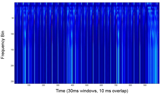
signal, an example is given in figure 2.4. In many speech processing algorithms, these
[image:20.612.143.462.292.479.2]responses are used to reconstruct the source signal.
Figure 2.4: Band-passed frequency response of a jazz song
The second piece of information of interest from this whole process is the Mel-frequency
cepstral coefficients themselves. The coefficients are generated by taking the log of the
band passed frequency response and calculating the discrete cosine transform (DCT) of
each intermediate signal. Typically, the Mel-frequency cepstral coefficients (Ci) of a frame
of audio data are the output from the DCT transform, given by equation 2.2 [7]
Ci = M X
j=1
mjCos
iπ
M (j−0.5)
i= 0,1,2, ...N; N < M;
where Yj is the output magnitude of the jth Mel-scale filtered signal and M is the
total number of Mel-scale filters in the filter bank analysis [7]. The resulting coefficients
represent the response of each particular frequency band at a particular window of time in
the audio sample. Therefore, for any window of time the relative response of the range of
frequencies audible to humans is given, with larger coefficients corresponding to a strong
feature for the window. The matrix output by determining the MFCC’s for an audio signal is
therefore accepted as a good statistical depiction of the original signal’s significant features
in the frequency domain. This technique has been widely used for feature extraction in
speech recognition as well as in applications processing digital music[18], [7], [9].
2.3
Principal Component Analysis
2.3.1
Theoretical Background
Principal component analysis (PCA) is a statistical transform for multidimensional data that
represents relevant patterns in data and outputs the information in a way that emphasizes
their similarities and differences [26]. Principal component analysis is used for reducing
dimensionality, identifying significant patterns, and has been used extensively in image and
audio processing [16] [26]. PCA does this by accounting for as much variance in the data
set as possible with each principal component. The process for computing the principal
components of a set of multidimensional data is based on the common statistical concepts
of variance, covariance and eigenvectors.
For a set of one dimensional data (dimensions can also be thought of as variables)
the spread, or range, of the information is commonly represented by standard deviation and
s2 =
Pn
i=1 Xi−X¯
2
(n−1) (2.3)
Because standard deviation and variance only operate on 1-dimensional data, a measure
is needed for multidimensional data sets; covariance is such a measure. It represents the
variance of dimensions of data with respect to each other. Therefore, the covariance of two
sets of observed data will determine how much the observations of one dimension change
with a given change in the other dimensions data. The equation for covariance of two
dimensions of dataX andY, withnobservations each is given in equation 2.4.
cov(X, Y) =
Pn
i=1 Xi−X¯
Yi−Y¯
(n−1) (2.4)
Because covariance represents a change in one dimension relative to a change in
an-other, then a positive covariance value indicates that as one set of data increases, the other
set of data will increase as well. Inversely, a negative covariance value indicates that as
one dimension increases the otherdecreases. Thus, a covariance value of zero means that
the two dimensions’ changes are statistically independent of each other and do not relate
linearly. This relationship can be evaluated for any number of dimensions, with each
di-mension of data being separately related to every other didi-mension. The information derived
from doing this is commonly organized into a covariance matrix containing the covariances
of all possible dimensional relationships. A covariance matrix for a set of data with three
dimensionsx,y, andz is shown in equation 2.5 [26].
C=
cov(x, x) cov(x, y) cov(x, z)
cov(y, x) cov(y, y) cov(y, z)
cov(z, x) cov(z, y) cov(z, z)
(2.5)
Down the main diagonal, you can see that the covariance value is between one of the
point is that since cov(a, b) = cov(b, a), the matrix is symmetrical about the main
diag-onal [26]. Calculating a covariance matrix for a high-dimensidiag-onal set of data is useful,
but difficult to interpret. Principle component analysis allows for dimension reduction and
interpretation of higher-level patterns and relationships in the data that are not
immedi-ately evident from the information contained in the covariance matrix. Yet, the covariance
matrix of relationships between each observed dimensions’ data is crucial to determining
the principal components of a set of data, which is completed with the calculation of the
eigenvectors and eigenvalues of the covariance matrix. Eigenvectors and eigenvalues can
be calculated by a number of different methods that solve the matrix algebra equation 2.6
C·V =V ·D (2.6)
whereDis the diagonal eigenvalue matrix andV is the associated eigenvector matrix
of the covariance matrix C [4]. Eigenvectors, also referred to as principal components,
latent dimensions, or principal features, represent the characteristic themes in a
multi-dimensional dataset. These eigenvectors will account for as much of the variance in the
original data set as possible. In fact, the German term eigen can be loosely translated
into ”peculiar” or ”characteristic” [4]. Each eigenvector will have with it one associated
eigenvalue in the diagonal matrix, where the eigenvector with the highest eigenvalue is
the n-length vector of an nby ncovariance matrix that represents the greatest amount of
variance in the entire data set (not just one of the original dimensions). Each subsequent
eigenvector with a gradually smaller eigenvalue, therefore, represents a slightly smaller
degree of variance in the data and is orthogonal to all other eigenvectors. Thus the
eigen-vectors of the covariance matrix, sorted by their eigenvalues, are the features or patterns
within the original data sorted by significance. Typically this information is returned by a
2.3.2
Process
The exact process for producing principal components is relatively straight forward,
be-ginning with subtracting the mean from each dimension of data for normalization. Then,
through whatever means is most convenient, calculate the covariance matrix for all of the
dimensions of the data. The last two steps are the evaluate the eigenvectors and
eigenval-ues of that covariance matrix, and simply sort the eigenvectors based on their associated
eigenvalues. With most modern statistical processing software this can be accomplished in
just a few function calls, or even just one. Because each eigenvector produced is
orthog-onal across all dimensions to the other principal components produced, the first principal
component identifies the vector that will account for the most variance in the data, and the
second component accounting for the most variance in the data in the second orthogonal
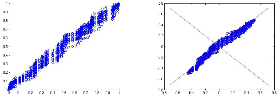
dimension. This is best visualized when a set of 2-dimensional data is plotted with it’s
calculated eigenvectors drawn over it as in figure 2.5. It is clear from the plots that the
eigenvectors represent the variance of the data, but not along the traditional x and y axes.
[image:24.612.115.560.448.605.2]Instead the vectors can also be used as axes to reorganize the data.
Figure 2.5: Raw data(left) and normalized data with eigenvectors superimposed(right)
One of the primary reasons for using an algorithm like PCA is to reduce dimensionality.
the very least, eigenvectors with an eigenvalue of zero are always considered insignificant,
and can be thrown out as they account for none of the variance in the data set. The retained
eigenvectors will represent the most significant patterns and features of the data with
mini-mal loss of information, but the amount of data has now been reduced making any further
calculations simpler and less computationally expensive.
2.3.3
Examples
There is a huge number of areas of research using principal component analysis, such as
economics, sociology, physics, and intelligent computing. They are particularly popular in
signal processing with images, video, and audio [26],[27], [25]. One of the most successful
applications of PCA in signal processing, has been the use of eigenfaces for identification,
recognition, and classification of humans in surveillance applications. This section will
describe the use of PCA for generating eigenfaces because it not only demonstrates the
significance of the process, but is a good visual representation of how PCA can represent
patterns and themes in data with a large number of dimensions.
The most effective algorithms for face detection and recognition have been the ones
that most closely model the actual performance of the human visual system’s ability to
quickly and accurately discern learned images. The use of a small set of representative
images, called eigenfaces, characterizes the principal components of a set of known faces.
The principal components of the known images represent a biologically inspired way of
representing the meaningful features of the set of pictures. These eigenfaces are also used
to reduce dimensionality of the data set to only include the most meaningful features of the
image set.
The process for generating eigenfaces is quite simple, beginning with a set of face
images of some uniform size (mbyn). The images are individually gray scaled and then
vectorized. The matrix of these image vectors (1 image per row) is considered the dataset
for principal component analysis. The images will each represent one dimension of mn
each display an eigenface when converted from theirmn-length eigenvector to anmbyn
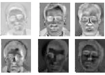
matrix as seen in figure 2.6.
Figure 2.6: Example eigenfaces
As you can see from the output images, there are clearly ghost-like facial features that
represent the variance in the facial features of all of the input images. The dimensionality
of the image information can be reduced by throwing out the eigenfaces with the lowest
eigenvalues because they will not represent a large amount of the original face data. In the
case of eigenfaces, each original image can still be almost entirely reconstructed through
some linear combination of the eigenfaces that remain. The coefficients of that linear
com-bination are the important information for this recognition technique. Figure 2.7 depicts
[image:26.612.221.399.160.287.2]the coefficients being used to reconstruct one of the original images.
Figure 2.7: Linear combinations of eigenfaces reconstruct original images
When new images are introduced to the system trained with these eigenfaces and
relative to the known eigenfaces. The coefficients are then compared to all the known sets
of coefficients to determine which known face matches the new face. This is a very basic
form of using eigenfaces for human face recognition and classification, and it has come
into widespread use in recent years. This is significant proof of the high-level, cognitive
processes that statistical transforms like this are capable of[27].
2.4
Independent Component Analysis
2.4.1
Introduction to ICA
Independent component analysis belongs to a class of blind source separation (BSS)
meth-ods for separating data into underlying components, where such data can take the form of
images, sounds, marketing data, or or stock market prices. ICA is based on the simple,
and physically realistic assumption that if different signals are from different physical
pro-cesses, then those signals are statistically independent[1]. Independent component analysis
takes advantage of the inverse of this assumption, which leads to a new assumption that is
logically un-sound but which works in practice. That assumption is that if statistically
inde-pendent signals can be extracted from signal mixtures then these extracted signals must be
from different physical processes[1]. ICA has been applied to problems in fields as diverse
as speech processing, brian imaging, audio and visual recognition, and stock market
pre-diction. Currently, research is being done with independent component analysis in many
different fields, and with its success in speech processing it is reasonable to say that it has
a large potential for more general acoustic separation and classification.
Independent component analysis is of interest to a wide variety of scientists and
engi-neers because it promises to reveal the driving forces behind a set of observed data signals,
including neurons, cell phone signals, stock prices, and voices[1]. The most common
ex-ample of using independent component analysis for blind source separation is thecocktail
party problem, where there are n people speaking at a party that is being recorded by n
algorithm, such as ICA, will be able to take thenmixtures of voices from the microphones
and separate out the individual voice signals from them. A depiction of how this problem
works can be found in figure 2.8. The microphone signals shown contain information from
each of the original input signals, which means that all of the different physical processes
[image:28.612.148.497.230.525.2]contribute to all of the mixtures.
Figure 2.8: Cocktail party problem using ICA[6]
It can be determined from the source signals that the amplitude of one at any given
point in time is completely unrelated to the others at that time. This indicates that they are
produced by two different, unrelated processes. Knowing that the sources are unrelated,
source signals by extracting the completely unrelated temporal signals of the two mixtures,
and it is true that these extracted signals are the original unrelated voices[1].
2.4.2
Theoretical Background
As stated above, independent component analysis (ICA) is a higher-order statistical
trans-form used in many of the same applications as principal component analysis. The biggest
difference between the two being that independent component analysis is an estimation of
components with a much stronger property then the components derived from PCA.
Prin-ciple component analysis will extract a set of signals that are uncorrelated. If the set of
mixtures in the cocktail party problem were microphone outputs then the extracted signals
from PCA would be a new set of voice mixtures, where ICA would extract the
indepen-dent signals from the mixtures. The indepenindepen-dent signals would be a set of single voices[1].
These representations seem to capture the essential structure of the data in many
applica-tions, including feature extraction and signal separation[14]. The theory of ICA is based
off of two primary equations seen in equation 2.8 and equation 2.9.
x=As (2.7)
s=W x (2.8)
x=
n X
i=1
aisi (2.9)
In the above equations x is the set of mixture signals, s is the independent source
signals, and A is the mixing matrix used to create x out of a linear combination of the
source signals as demonstrated by equation 2.9 whereaiis a column ofA. The variableW
is some unmixing matrix used to derive the source signals from the mixtures. This is the
purpose of an independent component algorithm, to properly estimate an unmixing matrix
that maximizes the nongaussianity, or statistical independence, of the source signals.
Higher-order processes like ICA use information on the distribution of x that is not
is contained in the covariance matrix, the distribution of x must not be assumed to be
Gaussian[15]. For more general families of density functions, the representation has more
degrees of freedom which the covariance matrix cannot account for. Much more
sophisti-cated higher-level algorithms must be employed for non-Gaussian random variables. The
transform defined by second-order methods like principal component analysis is not useful
for many purposes where dimension reduction in that sense is not needed. This is because
PCA neglects aspects of non-Gaussian data such as clustering and statistical independence
of the components[15]. Principle component analysis derives uncorrelated components,
which are not necessarily statistically independent. Statistically independent components
are by definition, uncorrelated as well.
One fact about blind source separation methods like ICA is that there must be at least
as many different mixtures of a set of source signals as there are source signals for the
algo-rithm to yield the best results[1]. A very basic example of this is shown in figure 2.11, with
the sawtooth and sine wave source signals. The first set of plots shows the source signals,
the second shows two arbitrary linear mixtures of the source signals, and the third shows
the extracted independent source signals after applying an ICA algorithm to the mixtures.
If there are more source signals then signal mixtures, blind source separation algorithms
have a great deal of difficulty extracting the source signals accurately, because the mixing
matrix will not be the same dimensions as the estimated unmixing matrix. Typically, the
number of signal mixtures is greater then the number of sources in practice. If this is the
case, then the number of source signals extracted can be reduced by either specifying the
number to extract or preprocessing the signal mixtures with a dimension reducing method
like principal component analysis[1].
As can be seen by the plots of the extracted source signals, there are some ambiguities
involved in performing independent component analysis: the order of the sources cannot
be determined, the original amplitude of the sources can not be extracted, and the original
phase of the signals cannot be determined either. None of these ambiguities, however,
Figure 2.9: Example source signals[22]
Figure 2.10: Example mixed signals[22]
Figure 2.11: Sources extracted using ICA[22]
the order of sources should be obvious, since the order in which the sources were added
can’t be determined as long as the mixing matrix A and source matrix s are unknown.
The second ambiguity is that the amplitude, or energies, of the sources is scaled by some
factor in the extracted sources. This is again becauseAandsare unknown and any scalar
multiplier in one of the sourcessicould always be canceled by dividing the corresponding
column ai of Aby the same scalar. The most intuitive way to fix the magnitude to some
value, is to assume that each has a variance equal to one. This leads to the third ambiguity
affecting the model. In most applications, however, these ambiguities are negligible or not
features of the sources taken into account at all, and thus insignificant[14].
2.4.3
Independence
It should be clear by now that independent component analysis is based on this concept
of statistical independence. Bascially, if two variables y1 and y2 are independent then
the value of one variable provides absolutely no information about the value of the other
variable[1]. For example, the temperature outside in Rochester, NY provides no
informa-tion about who wins the Iditarod. These two events are independent of each other. Another
example is tossing a coin. The result of each toss of the coin is independent of any other
tosses, so the probability of gettingheadson any number of tosses can be computed
with-out takingtailsinto account. This discussion of independence can be extended to the more
interesting example of speech. The probability that the amplitude of a voice signal slies
within an extremely small range around the valuestis given by the value of the probability
density function (pdf) ps(st) of that signal st[1]. Because speech signals spend most of
their time with a near-zero amplitude, the probability density function (pdf) of a speech
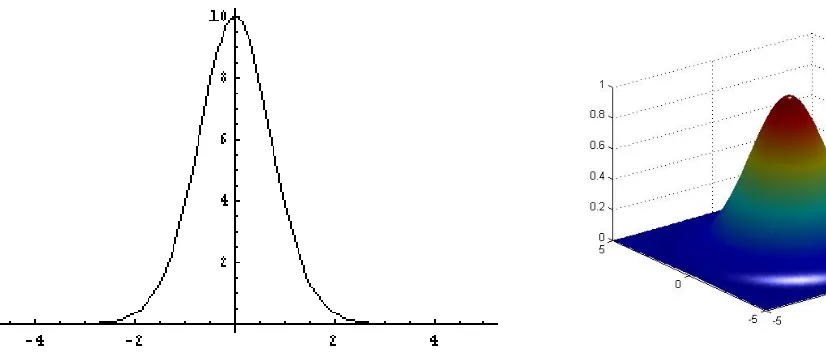
signal has a peak ats = 0, as shown in figure 2.12(left). The typical Gaussian probability
density function associated with Gaussian data is depicted in figure 2.12(right).
Now, we assume that two speech signalss1 ands2 from two different people are
inde-pendent. This implies that the joint probability is given by equation 2.10[1], where st is
the pair of values in the speech signals at time t represented by st = (st
1, st2). Therefore
the joint probability for all values of s is the joint pdf ps, and can be visualized for two
variables as shown in the left hand side of figure 2.12.
ps st
=ps1 st1
×ps2 st2
(2.10)
The pdfsps1andps2are known as the marginal pdfs of the joint pdfps. This probability
Figure 2.12: Speech joint PDF (left), Gaussian joint PDF (right)
variables s1 ands2 are independent. Just as the probability of flipping a coin and getting
headsmultiple times in succession can be obtained as the product of just the probability of
getting heads. Due to the fact that it is assumed that all values of each speech signal are
independent, the ordering of signal values is ignored[1].
The theory of statistical independence as applied to independent component analysis
suggests that a method of extracting the source signals from a set of mixtures is to find the
signals within the mixtures that are mutually independent, and therefore maximally
non-Gaussian. A measure of how independent signals are is needed to do this, permitting an
ICA algorithm to iteratively change the unmixing matrix in a way that increases the degree
of independence. Two such measures of independence are negentropy and kurtosis.
2.4.4
Measuring Independence
The principles behind an independent component analysis algorithm is the estimation of
sources and the maximization of statistical independence within the estimated sources. The
of the extracted sources. Referring back to the fundamental equations of independent
ponent analysis (see equations 2.8 2.9 2.9), to estimate just one of the independent
com-ponents, consider a linear combination of the xi mixture values from equation 2.9; where
y = wTx= P
iwixi, andwis a vector to be determined. Ifwwas one of the rows of the
inverse ofA, this linear combination would equal one of the independent components[14].
Even thoughwcan’t be determined exactly, an estimation that gives a good approximation
can be found[15].
To see how this leads to the basic principal of ICA estimation, a change of variables
is made, defining z = ATw. This gives y = wTx = wTAs = zTs. y is therefore
a linear combination of si, with weights (mixing matrix) given by zi. Since the sum of
even two independent random variables is more Gaussian than the original variables,zTs
is more Gaussian than any of the si and becomes the least Gaussian when it equals one
of the si[14]. Taking a vector w that maximizes the nongaussianity of wTx means that
wTx = zTs equals one of the independent components[14]. w has 2n local maxima,
two for each independent component, corresponding to si and −si[14]. To find several
independent components, we need to find all of these local maxima, which is not difficult
because the different independent components are uncorrelated, so we can always constrain
the search to the space that gives estimates uncorrelated with the previous ones[14].
These estimations require a measure of Gaussianity, or mutual dependence, with some
of the most common being Kurtosis or negentropy. Negentropy will be addressed first, and
is quite obviously based on the statistical concept of entropy. Entropy is a measure of the
uniformity of the distribution of a set of values, so that complete uniformity corresponds to
maximum entropy. If there exists a set of discrete signal values then the entropy of the set
depends on how uniform the values are, and the entropy of this set of variables is known
as the joint entropy[1]. An example of entropy for one variable and three variables can be
seen in figure 2.13. In the plot on the left, entropy is graphed against the probability of a
coin toss. When the probability of a coin toss isp= 0.5, the ability to predict it is minimal
Their entropy can be visualized as the degree of uniformity within the three dimensional
[image:35.612.105.518.162.319.2]plot shown.
Figure 2.13: Graph of entropy relative to probability of a coin toss[1](left), plot of 3 vari-ables with maximum entropy (right)
Entropy is the basic concept of information theory, the more ”random” or unpredictable
and unstructured the variable is, the larger its entropy. One way to calculate statistically
independent components is to find the unmixing matrix that maximizes the entropy across
all of the extracted signals. The differential entropy H of a random vectorywith density
f(y)is defined in equation 2.11[14].
H(y) =− Z
f(y)logf(y)dy (2.11)
A result of information theory is that a Gaussian variable has the largest entropy among
all random variables of equal variance[14]. This means that entropy could be used as a
measure of nongaussianity. Entropy is small for distributions that are clearly concentrated
on certain values. To obtain a measure of nongaussianity that is zero for a Gaussian variable
and always nonnegative, a slightly modified definition of differential entropy can be used,
J(y) = H(ygauss)−H(y) (2.12)
whereygauss is a Gaussian random variable of the same covariance matrix asy. Using
these properties, negentropy is always non-negative, and it is zero if and only if y has a
Gaussian distribution. The advantage of using negentropy, also called differential entropy,
as a measure of nongaussianity is that it is well justified by statistical theory. The problem in
using negentropy is, however, that it is computationally very difficult[14]. Approximations
for calculating negentropy in a much more computationally efficient manner have been
proposed as seen in equation 2.13. Varying the formula’s used for Gcan provide further
approximation with a minimal loss of information.
J(y)≈ p X
i=1
ki[E{Gi(y)} −E{Gi(v)}]2 (2.13)
This approximation of negentropy gives a very good compromise between the two
clas-sical measures of nongaussianity, kurtosis and negentropy. They are conceptually simple,
fast to compute, and still have desired statistical properties. This approximation is a good
place to introduce the other measure of nongaussianity, used in a method called projection
pursuit, kurtosis. The kurtosis of a signal is defined by equation 2.14, but in practice is
computed by equation 2.15[1].
K(y) =E
y4 −3 E
y2 2 (2.14)
K(y) =
1
N PN
t=1(y−y
t)4
1
N PN
t=1(y−yt) 22
−3 (2.15)
According to equation 2.14, since y is assumed to be of unit variance, the equation
simplifies to E{y4} − 3. Kurtosis is then a normalized version of the fourth moment
for a Gaussian random variable, whereas most nongaussian random variables will have a
nonzero kurtosis (either positive or negative). Random variables that have a negative
kurto-sis are called sub-Gaussian, and those with positive kurtokurto-sis are called super-Gaussian. The
magnitude of a signal’s kurtosis has been widely used as a measure of nongaussianity in
ICA. The main reason is its simplicity; computationally, kurtosis can be estimated simply
by using the fourth moment of the sample data, seen in equation 2.14[14]. The
compu-tationally practical equation for kurtosis (equation 2.15) has only one important term, the
numerator. The other terms are to take into account signal variance[1].
2.4.5
ICA and Projection Pursuit
Projection pursuit is a technique developed in statistics for finding interesting projections
of multidimensional data. These projections can then be used for optimal visualization
of the data, and for such purposes as density estimation and regression[14]. It has been
argued by [10] and others in the field of projection pursuit, that the Gaussian distribution
is the least interesting one, and that the most interesting projections are those that exhibit
the least Gaussian distribution. This is almost exactly what is done during the independent
component estimation of ICA, which can be considered a variant of projection pursuit[14].
The difference is that projection pursuit extracts one projected signal at a time that is as
nongussian as possible, whereas independent component analysis which extractsM signals
fromM signal mixtures simultaneously[1].
Specifically, the projection pursuit allows us to tackle the situation where there are less
independent components si than original variables xi. However, it should be noted that
in the formulation of projection pursuit, no data model or assumption about independent
components is made[14]. In ICA models, optimizing the nongaussianity measures
pro-duces independent components; if the model does not hold, then the projection pursuit
2.4.6
Preprocessing
Before employing any independent component algorithm, it is most often useful to do
some preprocessing on the data set. This section will briefly describe a few preprocessing
techniques commonly used in conjunction with ICA, such as centering and whitening. The
most basic and necessary preprocessing is to centerxby subtracting its mean to makexa
zero-mean variable. This preprocessing is made solely to simplify the ICA algorithms, but
they will calculate the actual mean otherwise. After estimating the mixing matrix A with
centered data, we can complete the estimation by adding the mean vector ofs back to the
centered estimates of s. The mean vector of sis given byA−1m, wherem is the mean
that was subtracted in the preprocessing[14].
The other useful preprocessing tool is data whitening, which occurs before performing
the independent component analysis algorithm, but after centering. The observed vector
x is linearly transformed so that it is white. A vector is white when its components are
uncorrelate and their variances equal unity[14]. The result of doing this is a data vector
whose covariance matrix is equal to the identity matrix, given by equation 2.16.
Ex˜x˜T =I (2.16)
One popular method for whitening is to use the eigen-value decomposition (EVD) of
the covariance matrix. Whitening transforms the mixing matrix into a new one, A˜giving
equation 2.17 (see [14] for proof).
˜
x=ED−12ETAs = ˜As (2.17)
Whitening reduces the number of parameters that need to be estimated, fromn2
param-eters of the original matrix Aton(n−1)/2parameters of the orthogonal mixing matrix
˜
A[14]. Whiteneing essentially reduces the complexity of the problem that has to be
2.4.7
FastICA Algorithm
The FastICA algorithm was developed at the Laboratory of Information and Computer
Sci-ence in the Helsinki University of Technology by Hugo Gvert, Jarmo Hurri, Jaakko Srel,
and Aapo Hyvrinen. The FastICA algorithm is a highly computationally efficient method
for performing the estimation of ICA. It uses a fixed-point iteration process that has been
determined, in independent experiments, to be 10-100 times faster than conventional
gradi-ent descgradi-ent methods for ICA. Another advantage of the FastICA algorithm is that it can be
used to perform projection pursuit as well, thus providing a general-purpose data analysis
method that can be used both in an exploratory fashion and for estimation of independent
components (or sources)[3].
The basic process for the algorithm is best first described as a one-unit version, where
there is only one computational unit with a weight vectorwthat is able to update by a
learn-ing rule. The FastICA learnlearn-ing rule finds a unit vectorw such that wTxmaximizes
non-gaussianity, which in this case is calculated by the approximation of negentropyJ wTx
.
The steps of the FastICA algorithm for extracting a single independent component are
out-lined below.
• Take a random initial vectorw(0)of norm 1, and letk= 1
• Let w(k) = E
xw(k−1)T x
3
− 3w(k−1). The expectation can be
esti-mated using a large sample ofxvectors (say, 1,000 points).
• Dividew(k)by its norm.
• If w(k)Tw(k−1)
is not close enough to 1, let k = k + 1and go back to step 2.
Otherwise output the vectorw(k).
After starting with a random guess vector forw, the second step is the equation
find-ing maximum independence, with the third checkfind-ing the convergence to a local maxima.
Derivations of these steps can be found in [13]. The final w(k) vector produced by the
of blind source separation, this means that w(k) extracts one of the nongaussian source
signals from the set of mixturesx. This set of steps only estimates one of the independent
components, so it must be runntimes to determine all of the requested independent
com-ponents. To guard against extracting the same independent component more then once, an
orthogonalizing projection is inserted at the beginning of step three, changing it to the item
below.
• Letw(k) = w(k)−W WTw(k)
Becuase the unmixing matrixW is orthogonal, independent components can be
esti-mated one by one by projecting the current solution w(k)on the space orthogonal to the
columns of the unmixing matrixW. The matrixW is defined as the matrix whose columns
are previously found columns of W. This decorrelation of the outputs after each
itera-tion solves the problem of any two independent components converging to the same local
maxima[13].
The convergence of this algorithm iscubic (see [13] for proof), which is unusual for
an independent component analysis algorithm. Many algorithms use the power method,
and converge linearly. The FastICA algorithm is also hierarchical, allowing it to find
inde-pendent components one at a time instead of estimating the entire unmixing matrix at once.
Therefore, it is possible to to estimate only certain independent components with FastICA if
there’s enough prior information known about the weight matrices[13]. The FastICA
algo-rithm was developed to make the learning of kurtosis faster, and thus provide a much more
computationally efficient way of estimating independent components. It’s performance and
theoretical assumptions have been proven in independent studies and [13], and given cause
for it to be used in the development of a process that will quickly evaluate and separate
the high-level components of acoustic information. The originally developed FastICA
al-gorithm Matlab implementation can be found at http://www.cis.hut.fi/projects/ica/fastica/,
2.4.8
Temporal vs. Spatial ICA
For all of the independent component analysis examples given so far, a set ofM temporal
signal mixtures is measured over N time steps, andM temporal source signals are
recov-ered so that each source signal is independent over time of the others[1]. When considering
time-domain signals, each row of the data matrixxis a temporal signal over time. The data
can also be viewed as the transpose where each column of the original matrixxis a spatial
signal at one point in time. When the rows of the matrix x are treated as mixtures over
time, ICA produces temporal independent components, but treating the columns as
mix-tures produces spatial independent components[1]. Independent component analysis can
therefore be used to maximize independence over time or space. An example of each type
of independent component analysis can be given in speech signal separation (cocktail party
problem) for temporal ICA and functional magnetic resonance imaging (fMRI) for spatial
ICA. For the rest of this section comparing the two forms of ICA, sICA will be used to
refer to spatial independent component analysis and tICA will be used to refer to temporal
independent component analysis[1].
The problems solved by tICA and sICA are, for the most part, the same and the
algo-rithms used are certainly the same. The only difference is in the orientation of the mixture
matrix passed to the ICA algorithm, and whether the extracted components are considered
independent over time or over space.
tICA
Temporal independent component analysis is used to extract each temporal source signal
from the mixtures at each point in time, but only one point in space. This is much better
ex-plained through the example of blind source separation to solve the cocktail party problem.
Eachn-length mixture signal comprises a row of the overall mixture matrix and can then be
viewed as a variable, withnobservations at successive points in time[1]. Assumingm
observed point in time producing an n byn unmixing matrix. The unmixing matrix
cou-pled with the mixture signals will yield an mbyn independent component matrix, where
each of the m rows are mutually independent temporal signals. Each of the independent
temporal components defines how a specific source contributes to the temporal sequence
of mixtures at each point in time.
sICA
Spatial independent component analysis can be interpreted as each signal being a mixture
of underlying source signals, and a source vector as a spatial sequence measured at a single
point in time. This is in direct contrast with tICA, which considers temporal mixtures or
underlying temporal source signals measured over time and at one point in space[1]. Using
the same example as tICA, but with the mixture matrix transposed (i.e. n rows and m
columns) to place each observation of the temporal signals in a row, sICA will determine
the set of independent spatial source signals. Thus, sICA would estimate an m by m
unmixing matrix so that the extracted spatial signals are mutually independent. This will
output a set ofm-length independent components that are independent over space of spatial
patterns at all other points in time[1].
2.4.9
Use in Cognitive Modeling
As stated earlier, independent component analysis has been used in many applications in
the field of computer vision and signal processing because of its success in identifying
underlying components and patterns in very complex, multi-dimensional data. ICA has
found uses in many different areas of cognitive processing, such as neuroscience, statistical
analysis, physics, audio signal processing, and image and video processing. This section
will briefly outline some of the applications for using independent component analysis to
develop cognitive processes, and introduce some more of the ideas that make up the basis
for this research.
magnetic resonance images (fMRI) and Magnetoencephalography (MEG). These are both
noninvasive techniques by which the activity of the cortical neurons can be measured with
a very good temporal resolution and moderate spatial resolution. When using an MEG
record, the user will most likely be faced with the problem of extracting the principal
fea-tures of the neuromagnetic signals adjusting for the presence of artifacts. In [12], the
authors introduced a new method to separate brain activity from artifacts using
indepen-dent component analysis, specifically sICA[14]. The approach is based on the assumption
that the brain activity and the artifacts are anatomically and physiologically separate
pro-cesses, and this separation is reflected in the statistical independence between the magnetic
signals generated by those processes. ICA has been proven effective in extracting
spa-tially independent features of interest from the MEG and fMRI records[14] [12]. This is
an application of sICA for a process that is not intuitive to human beings, like many of the
applications with images and sound are.
In the statistical analysis world, more often then not associated with commerce and
fi-nance, it is a tempting alternative to try independent component analysis on financial data.
There are many situations in which parallel time series are available, such as currency
ex-change rates or daily returns of stocks, that may have some common underlying factors.
ICA might reveal some driving factors of the data that otherwise remain hidden. The
as-sumption of having some underlying independent components in this specific application
is not unrealistic[14]. For example, factors like seasonal variations due to holidays and
annual variations, and factors having a sudden effect on the purchasing power of the
cus-tomers can be expected to have an effect on all markets. Such factors can be assumed to
be roughly independent of each other. Depending on the policy and skills of the individual
retailer, such as advertising efforts, the effect of the factors in the overall market on
partic-ular businesses are slightly different. By ICA, it is possible to isolate both the underlying
factors and the effect weights, therefore also making it possible to group the stores on the
basis of their managerial policies using only the cash flow time series data[14].
the ”gist” of a set of natural images and group them based on their higher level features.
Independent component analysis has two quite common roles in image processing,
extract-ing low-level features, and matchextract-ing images to the patterns in them. In this experiment, a
set of natural images were passed through independent component analysis to extract the
independent features throughout the entire data set of images. In the next step, the images
were individually passed through ICA to extract the independent feature specific to that
image[17]. This allowed the images to be grouped together based on which of the features
generated in the first step best matched features from the second. This leads to
content-based grouping of images whose high level features are extremely similar. Results of this
[image:44.612.130.493.326.496.2]implementation can be seen in the image groupings below.
Figure 2.14: Grouping of underbrush images(left) and horizons(right) [17]
A good survey of independent component analysis applications can be found in [16]
where principal and independent component analysis is used to demonstrate possible
use-ful applications in text analysis, analyzing social networks, and musical genre analysis.
This work developed processes for various forms of text, social network, and musical genre
analysis using principal component analysis. The eigenvectors generated, and their
rela-tionships to each other were shown to exhibit characteristics of statistical independence.
to exploit this independence for exploring automatic text content analysis, social network
understanding, and musical genre classification. It is the processes posed in this work that
have, in great part, lead to the research developed in this thesis. The idea of developing a
process to analyze music files in order to automatically determine their respective genres is
also explored in [24] [20] [18]. This work will attempt to develop a process, based on
in-dependent component analysis, to automatically segregate acoustic information, including
Chapter 3
Cognitive Model
3.1
Previous Work
The basis for this thesis research has come from the current significance of the problems
that exist in automatically labeling, categorizing, and managing digital media expressed in
the introduction. Extensive research was done to explore the advancements and previous
work that had been done in this area. I looked into the subject matter, background theory,
processes, and signal processing techniques being used to address these issues and develop
a specific area of research to focus the novel work presented here. After a great deal of
searching, it was determined that a quick, computationally efficient process using some
common preprocessing method and independent component analysis to separate general
acoustic information did not yet exist. This section will discuss the previous work done in
this area, and the extensions to that work used to comprise the process developed in this
thesis.
In previous works in the area of acoustic feature extraction and modeling, it has been
shown that Mel-frequency cepstral coefficients are a good audio preprocessing step to
ex-tract general low-level features from music and speech signals [16] [18]. The windowed
MFCC’s create a smoothed signal that highlights strong temporal frequency responses
without losing information from the original signal. Also, reasonable decision time
hori-zon’s have been determined in similar methods used for audio classification, which attempt
of the entire signal’s classification[20]. This is an important feature in developing a signal
processing algorithm. In practice, an algorithm developed for the automatic organization
of digital media should execute in a timely and efficient manner. To analyze the entire
audio signal, which can vary greatly in length, would take an excessive amount of time.
It’s also intuitive to the end goal of the process, because humans can determine the general
classification of an audio signal after hearing only a short portion of it. To only use a small
portion of the signal in classification is not only biologically accurate, but computationally
efficient as well.
However, the Mel-frequency cepstral coefficients of a sample audio signal is not a high
enough abstraction of the original signal to perform classification. MFCC’s are effectively
coefficients of a signal’s relative response to certain frequency bands. Therefore, using
another form of signal processing to find the higher-level temporal themes in the signal
would give a good representation of the temporal patterns and components of the input
signals. This representation of patterns across high dimensional data will yield a set of
themes that should be similar across signals within the same class and distinct across signals
[image:47.612.108.585.454.626.2]of different classes.
Figure 3.1: Music preprocessing results from [16] (left), and recreated results (right)
different genres of music would produce a relatively unique set of characteristic themes.
As can be seen in figure 3.1, the author’s original work using principal component analysis
showed that on some higher dimensions, the music occupied different spaces and even
displayed some statistical independence. To gain some understanding of these results and
the feasibility of the work, I have recreated some simple results using PCA and placed
them next to the plot of the original work. This work, as well as the work of others in
the area of acoustic classification has shown that the use of statistical transforms like PCA
and ICA, for signal processing, is a reasonable means for extracting unique and significant
patterns from acoustic data [16] [24] [20]. It was proposed in [16] that because the features
of different genres of music showed signs of statistical independence, that the use of a
combination of Mel-frequency cepstral coefficients and independent component analysis
in classifying music by genre and sub-genre would be a good extension to the concepts
they had demonstrated. This extension into developing a process for separating classes of
music,
![Figure 2.1: Auditory Cortex Model[2]](https://thumb-us.123doks.com/thumbv2/123dok_us/118890.11514/16.612.137.479.104.328/figure-auditory-cortex-model.webp)
![Figure 2.2: Human cochlea, which reacts in different areas to different frequencies of sound[2]](https://thumb-us.123doks.com/thumbv2/123dok_us/118890.11514/18.612.198.425.101.298/figure-human-cochlea-reacts-different-areas-different-frequencies.webp)
![Figure 2.3: MFCC process(left)[5] and Mel-scale filter bank(right)[22]](https://thumb-us.123doks.com/thumbv2/123dok_us/118890.11514/19.612.125.505.99.273/figure-mfcc-process-left-mel-scale-lter-right.webp)
![Figure 2.8: Cocktail party problem using ICA[6]](https://thumb-us.123doks.com/thumbv2/123dok_us/118890.11514/28.612.148.497.230.525/figure-cocktail-party-problem-using-ica.webp)
![Figure 2.9: Example source signals[22]](https://thumb-us.123doks.com/thumbv2/123dok_us/118890.11514/31.612.181.439.105.472/figure-example-source-signals.webp)
, plot of 3 vari-ables with maximum entropy (right)](https://thumb-us.123doks.com/thumbv2/123dok_us/118890.11514/35.612.105.518.162.319/figure-graph-entropy-relative-probability-ables-maximum-entropy.webp)