Aerosols and Chemistry in the Planetary Atmospheres

(1)

Aerosols and Chemistry in the

Planetary Atmospheres

Thesis by

Xi Zhang

In Partial Fulfillment of the Requirements for the Degree of

Doctor of Philosophy

CALIFORNIA INSTITUTE OF TECHNOLOGY Pasadena, California

2013

(2)

(3)

To my parents and

(4)

ACKNOWLEDGEMENTS

Following Chinese tradition, I would first like to thank my parents, my sister, and her family. Their endless love reached across the Pacific Ocean and has never ceased to comfort me and cure me of my homesickness in the last five and a half years. It is to them that this dissertation is dedicated.

I owe my most sincere gratitude to my Ph.D. advisor Yuk Yung. Without him, this thesis is not possible. Two thousand years ago, Confucius described a Chinese gentleman as having “three varying aspects: seen from afar, he looks severe, when approached he is found to be mild, when heard speaking he turns out to be incisive.” Yuk is a gentleman. He is the most sincere person I have ever met. As far as I know, he is the only Ph.D. advisor who takes students to the supermarket to shop for groceries (please ask Mike Wong for details) and fixes their cars (please ask me for details). He cares about the students. Thus, he not only passes on to them his scientific knowledge and research methods, but he also inspires and encourages them through his everyday life as a unity of knowledge and practice. I believe the latter is inherited from the traditional Chinese scholars that came after Confucius. He taught me not only how to accelerate but also how to break, and why the most important attributes are judgment and vision. Also, I must thank Shaumay, Yuk’s wife, for her delicious dishes that she shared with us every year when we had parties at their house.

I would also like to thank John Seinfeld. His aerosol class might be my most productive class at Caltech, as my class project was quickly published and eventually became the first chapter of my thesis. I learned a lot from his efficiency and physical insights during my collaboration with him.

(5)

information mined from planetary data in a reasonable way. Robert West and his insistence on the research approach finally led me to the light at the end of the tunnel, although at the beginning I thought it was an impossible task. Run-lie Shia’s physical intuition and insightful comments are always appreciated. A complete list is not possible, although I would like to thank as many as I can. They are Mark Allen, Adam Showman, Spyros Pandis, Patrick Irwin, Donald Shemansky, Mao-Chang Liang, Franklin Mills, Denis Belyaev, Raul Morales-Juberias, Timothy Dowling, Christopher Parkinson, Joseph Ajello, Julie Moses, Leigh Fletcher, Glenn Orton, Roger Yelle, Frank Montmessin, Jean-Loup Bertaux, Oded Aharonson, Victoria Meadows, Javier Martin-Torres, Don Banfield, as well as the young rising stars: Mike Line, Peter Gao, Joshua Kammer, and Cheng Li. Clearly, the US planetary science community is a good example of a mature scientific field.

I am also grateful for the support from the planetary science option staff, especially from Irma Black and Margaret Carlos. Special thanks also go to Mike Black and Scott Dungan for having resolved my numerous computer problems. I must also thank Shawn Ewald for his advice on IDL programming, Mimi Gerstell for having corrected the grammar errors in my papers, and Irene Chen for having translated my LaTex manuscript into the Microsoft Word format.

(6)

I would like to thank the friends who shared the joys of their family with me: Runqiang and Yu, Zhaoyan and Tian, Na and Pengcheng, Wei and Rui, Guanglei and Mingyuan (and their beautiful twins!), Hank and Eileen, Ting and Fan, and Lijun and Yun. May their love shine warmly forever.

I devote my thesis to Haogang Xiao, my dearest brother in the heavens; I will stop blaming you for leaving us alone. Yunfeng and Jiayu, let us carry on his unfinished dreams together.

(7)

ABSTRACT

This dissertation is devoted to studying aerosols and their roles in regulating chemistry,

radiation, and dynamics of planetary atmospheres. In chapter I, we provided a

fundamental mathematical basis for the quasi-equilibrium growth assumption, a

well-accepted approach to representing formation of secondary organic aerosols (SOAs) in

microphysical simulations in the Earth’s atmosphere. Our analytical work not only

explains the quasi-equilibrium growth, which emerges as a limiting case in our theory,

but also predicts the other types of condensational growth, confirmed by the recent

laboratory and field experiments. In chapter II, we presented a new photochemical

mechanism in which the evaporation of the aerosols composed of sulfuric acid or

polysulfur on the nightside of Venus could provide a sulfur source above 90 km. Our

model results imply the enhancements of sulfur oxides such as SO, SO2, and SO3. This is

inconsistent with the previous model results but in agreement with the recent

ground-based and spacecraft observations. In chapters III and IV, we developed a nonlinear

optimization approach to retrieve the aerosol and cloud structure on Jupiter from the

visible and ultraviolet images acquired by the Cassini spacecraft, combined with the

ground-based near-infrared observations. We produced the first realistic spatial

distribution of Jovian stratospheric aerosols in latitudes and altitudes. We also retrieved

the stratospheric temperature and hydrocarbon species based on the mid-infrared spectra

from the Cassini and Voyager spacecrafts. Based on the above information, the accurate

(8)

obtained, revealing a significant heating effect from the polar dark aerosols in the high

latitude region and therefore a strong modulation on the global meridional circulation in

the stratosphere of Jupiter. In chapter V, we study the transport of passive tracers, such as

aerosols, acetylene (C2H2) and ethane (C2H6) in the Jovian stratosphere, using both

analytical and numerical approaches. We established several benchmark analytical

solutions for the coupled photochemical-advective-diffusive system to understand its

basic behaviors under different assumptions. A numerical two-dimensional chemical

transport model is applied to Jupiter, and the effects of eddy mixing process and

(9)

List of Figures

1.1. Analytical solution of diffusion-limited growth in an open system ... 18

1.2. Analytical solution of quasi-equilibrium growth in an open system ... 18

1.3. Evolution of the aerosol distributions in a closed system: case 1 ... 20

1.4. Evolution of the aerosol distributions in a closed system: case 2 ... 20

1.5. Evolution of the aerosol distributions in a general system: case 1 ... 21

2.1. Atmospheric profiles on Venus ... 31

2.2. VMR profiles of the oxygen species from model A ... 34

2.3. VMR profiles of the hydrogen species from model A ... 34

2.4. VMR profiles of the chlorine species from model A ... 35

2.5. VMR profiles of the chlorine-sulfur species from model A ... 35

2.6. VMR profiles of the elemental sulfur species from model A ... 36

2.7. VMR profiles of the nitrogen species from model A ... 36

2.8. VMR profiles of the sulfur oxides from model A ... 37

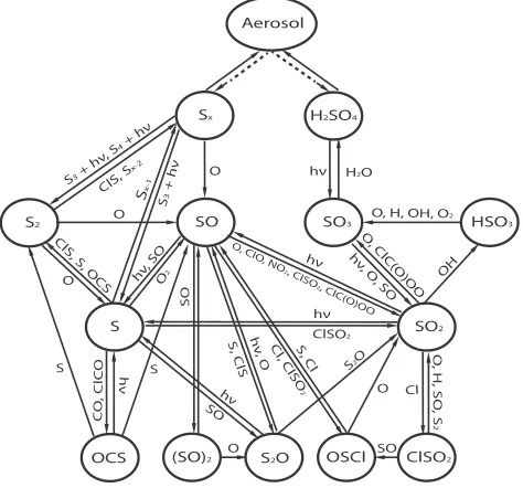
2.9. Important chemical pathways for sulfur species. ... 39

2.10. Important production and loss rates for sulfur oxides from model A ... 40

2.11. Comparison between model A and model B ... 42

2.12. Important production and loss rates for sulfur oxides from model B ... 43

2.13. Sensitivity studies based on model A. ... 47

2.14. Production rate profiles of H2SO4 and Sx ... 48

2.15. Important timescales for S2, S3 and S4 ... 55

2.16. Sulfur flux flow in the upper atmosphere of Venus ... 59

3.1. Summary of the previous measurements on Jovian stratosphere ... 68

3.2. Ensemble Retrieval results from Cassini CIRS observations ... 71

3.3. A typical set of retrieval results from Cassini CIRS data ... 73

(14)

3.5. A typical set of retrieval results from Cassini IRIS data ... 76

3.6. Infrared cooling rate based on Cassini data ... 81

3.7. Non-LTE model results ... 85

3.8. Zonally averaged stratospheric cooling rate map ... 87

3.9. Spectrally resolved CH4 heating rate ... 89

3.10. Globally averaged CH4 heating rates ... 90

3.11. Instantaneous global energy balance plot of Jovian stratosphere ... 91

3.12. Sensitivity test of the CIRS cooling rate in the lower stratosphere ... 93

3.13. Important timescales for Jovian stratosphere ... 101

4.1. Total gas optical depth including CH4 and H2-H2 CIA at 100 mbar ... 108

4.2. Comparison of the best solutions from NIR spectra ... 109

4.3. Retrieved aerosol map on Jupiter ... 111

4.4. Sample images from three ISS filters ... 114

4.5. Cartoon of the retrieval model structure ... 115

4.6. UV/NIR extinction ratios and aerosol NIR phase functions ... 120

4.7. Retrieval results in the equatorial region from the MIE model ... 124

4.8. Retrieval results in the mid latitude (45! N) from the AGG model ... 126

4.9. Retrieval results in the mid latitude (65! N) from the AGG model ... 127

4.10. Refractive index of aerosols ... 128

4.11. Summary of important retrieved parameters as function of latitude ... 130

4.12. Retrieved phase functions for aerosols and clouds ... 132

4.13. Total aerosol column density and mass loading ... 133

4.14. Profiles of particle number density and heating rate ... 135

4.15. Spectrally resolved aerosol and CH4 heating rates. ... 136

4.16. Globally averaged radiative heating rates ... 137

4.17. Zonal averaged solar heating rate map ... 138

4.18. Zonal averaged net radiative forcing map ... 139

4.19. Instantaneous global energy balance of Jovian stratosphere ... 140

4.20. Sensitivity test for the aerosol heating rates ... 142

(15)

4.22. Bond albedo of Jupiter for each latitude ... 145

4.23. Energy flows in the atmosphere of Jupiter ... 147

5.1. Simulated hydrocarbon profiles ... 155

5.2. Profiles of eddy diffusivity and molecular diffusivity ... 155

5.3. Analytical and numerical CH4 profile ... 158

5.4. Analytical and numerical C2H6 profile ... 159

5.5. Analytical and numerical C2H2 profile ... 162

5.6. Analytical CH4 profiles from the cases with and without wind ... 164

5.7. Analytical C2H6 profiles from the cases with and without wind ... 165

5.8. Analytic mass stream functions ... 174

5.9. Analytical and numerical solutions for cases I and case II ... 175

5.10. Analytical and numerical solutions for case III ... 177

5.11. Analytical and numerical solutions for case IV ... 179

5.12. Analytical and numerical solutions for case V ... 179

5.13. Analytical and numerical solutions for case VI ... 180

5.14. Analytical solutions for the zonal transport cases ... 183

A.1. Optical Properties of aerosols in the Venus model ... 186

A.2. Spectral actinic flux in the middle atmosphere of Venus at 45° N ... 187

A.3. Aerosol profiles on Venus ... 198

A.4. Equilibrium H2O mixing ratio contours ... 201

A.5. Volume mixing ratio profiles of H2SO4 and H2SO4!H2O ... 203

A.6. Saturated vapor volume mixing ratio profiles of Sx allotropes ... 205

A.7. H2SO4 cross sections ... 206

B.1. Test cases for cooling rates defined in layers ... 217

B.2. Test cases for cooling rates defined at levels ... 217

B.3. Test cases of upward IR fluxes !! _! _{... 218}

(16)

List of Tables

2.1. Boundary conditions of the Venus photochemical model. ... 33

2.2. Summary of models A and B ... 44

3.1. Collisional deactivation rates (s!1_{) at 1 µbar and 296 K ... 84}

4.1. Selected Cassin ISS images for aerosol retrieval ... 113

4.2. Typical DHG model results for latitude 0!, 45!!N, and 65!!N ... 121

4.3. Best-fitted MIE model results for the low latitudes (40!!S-25!!N) ... 123

4.4. Best-fitted AGG model results ... 125

4.5. Best-fitted AGG model results for north and south polar regions ... 129

A.1. Photolysis Reactions on Venus ... 189

(17)

Preface

In the revolution of the universe are comprehended all the four elements, and this being circular and having a tendency to come together, compresses everything and will not allow any place to be left void. Wherefore, also, fire above all things penetrates everywhere, and air next, as being next in rarity of the elements; and the two other elements in like manner penetrate according to their degrees of rarity. For those things which are composed of the largest particles have the largest void left in their compositions, and those which are composed of the smallest particles have the least. And the contraction caused by the compression thrusts the smaller particles into the interstices of the larger. And thus, when the small parts are placed side by side with the larger, and the lesser divide the greater and the greater unite the lesser, all the elements are borne up and down and hither and thither towards their own places; for the change in the size of each changes its position in space. And these causes generate an inequality which is always maintained, and is continually creating a perpetual motion of the elements in all time.

_{Timaeus, Plato, 427~347 BC}

(18)

In this dissertation, I selected several publications related to aerosols and their roles in planetary atmospheres. Aerosols are the condensed phases in the atmospheres. They could be solid (e.g., ice crystals and dusts on Mars) or liquid (e.g., sulfuric acid droplets on Venus), or some semi solid phase between them (e.g., polysulfur on Venus). Aerosols could come from many sources. For example, the primary aerosols on Earth are directly emitted from the surface (e.g., sea salt), while the secondary aerosols in the atmosphere are produced by the gas-phase chemical processes. The formation mechanisms of aerosols and their interactions with gas and radiation field are very complicated. Readers are encouraged to consult chapters 8~15 in Seinfeld and Pandis (2006) for our current understanding on aerosols. Aerosols are not only a challenging problem on many planets, but also, or more importantly, aerosol radiative forcing contributes the greatest uncertainty to the Earth’s climate predictions according to the recent 2007 IPCC (Intergovernmental Panel on Climate Change) report.

This dissertation is multidisciplinary, trying to elaborate on different aspects on aerosol sciences for different planetary atmospheres. In the following chapters, I focus on several key questions, including how do they form on Earth (chapter I), how do they interact with other atmospheric species on Venus (chapter II), how to determine their properties and distributions on Jupiter (chapter IV), how do they influence the radiative energy distributions on Jupiter (chapter III and IV), and how do the atmospheric circulation and mixing processes shape the tracer (including aerosols) distributions in general and specifically on Jupiter (chapter V). The supplementary materials of chapter II and III are summarized in Appendices A and B, respectively.

(19)

Chapter I

Diffusion-Limited versus Quasi-Equilibrium Aerosol Growth

*

That is Dao of heaven; it depletes those who abound, and completes those who lack.

!! Lao Tsu, Ancient China

Summary

Condensation of gas-phase material onto particulate matter is the predominant route by which atmospheric aerosols evolve. The traditional approach to representing formation of secondary organic aerosols (SOAs) is to assume instantaneous partitioning equilibrium of semivolatile organic compounds between gas and particle phases. Growth occurs as the vapor concentration of the species increases owing to gas-phase chemistry. The fundamental mathematical basis of such a condensation growth mechanism (quasi-equilibrium growth) has been lacking. Analytical solutions for the evolution of an organic aerosol size distribution undergoing quasi-equilibrium growth and irreversible diffusion-limited growth are obtained for open and closed systems. The quasi-equilibrium growth emerges as a limiting case for semivolatile species condensation when the rate of change of the ambient vapor concentration is slow compared with the rate of establishment of local gas-aerosol equilibrium. The results suggest that the growth mechanism in a particular situation might be inferred from the characteristics of the evolving size distribution. In certain conditions, a bimodal size distribution can occur during the condensation of a single species on an initially unimodal distribution.

*_{Appeared as: Zhang, X., Pandis, S.N., Seinfeld, J.H., 2012. Diffusion-limited versus}

(20)

1.1.Introduction

The size distribution of atmospheric aerosols is controlled largely by gas-to-particle conversion, and the characteristics of the evolution of the size distribution are indicative of the nature of the to-particle conversion process. The mode of condensation of gas-phase organic species onto ambient aerosols is of particular interest. In theory, the rate of condensation of a vapor molecule on a particle is controlled by the difference between the ambient partial pressure of the substance and its equilibrium vapor pressure over the particle surface (Seinfeld and Pandis 2006). Under typical atmospheric conditions, the

characteristic timescale for gas-phase diffusion to establish a steady-state pro"le around a

particle is generally less than 10-3 _{s (Seinfeld and Pandis 2006). Therefore, at any instant of}

time, the concentration pro"le of the species in the vicinity of the particle is established by steady-state molecular diffusion. Once the equilibrium vapor pressure of the condensing species over the particle surface becomes equal to the ambient partial pressure, equilibrium is established between the gas and aerosol phases. If the ambient partial pressure changes slowly relative to the timescale over which the gas-aerosol equilibrium is established, the particle grows (or evaporates) accordingly. The rate of particle growth in this situation is then controlled by the (slower in general) rate of change of the equilibrium vapor pressure over the particle surface. This situation can be referred to as volume-limited or quasi-equilibrium growth. The traditional rate of condensation that depends on the difference between the ambient partial pressure and the vapor pressure over the particle surface can be termed diffusion-limited (or kinetic) condensation. If the equilibrium vapor pressure of the condensing species is zero or practically zero, then the diffusion-limited growth is irreversible.

(21)

its volume fraction (as compared with the total particle volume) of this group. In this application, it was assumed that the particles were mainly organic, so the organic fraction is similar to the total volume fraction. Riipinen et al. (2011) evaluated both approaches to representing organic condensation on the evolution of ambient aerosol size distributions, by comparing predicted versus observed growth rate of freshly nucleated particles. They assumed that the organic species consisted of a low-volatility species that condenses kinetically on the surface area distribution and a semivolatile species that instantaneously reaches gas-particle equilibrium with the aerosol volume distribution. In a comparison of predicted and observed growth rates, the best agreement was achieved when at least 50% of the organic aerosol was assumed to condense via the irreversible kinetic route. Thus, the work of Riipinen et al. (2011) work suggested that the evolution of atmospheric aerosol size distribution owing to organic species condensation exhibits features characteristic of both traditional irreversible diffusion-limited mass transfer and a process in which growth depends on the volume of condensed species. A characteristic of the latter mechanism is that the greater the amount of condensed absorbing material, the greater is the capacity for absorption of vapor.

Recent work illustrated the potential role of different mechanisms of particle growth in the formation of secondary organic aerosol (SOA). Perraud et al. (2012) reported studies of particles formed in the simultaneous oxidation of #-pinene by !! and !"!. The !"!

reaction with #-pinene led to organic nitrates, which typically are more volatile than the

products of ozonolysis. In separate experiments, organic nitrate vapor products from the

reaction of #-pinene and !"! are exposed to liquid polyethylene glycol (PEG) particles.

Uptake by the PEG droplets was shown to be consistent with gas-particle partitioning equilibrium. Uptake of the same nitrate products by the SOA formed by the ozonolysis of

#-pinene, however, was shown to behave consistent with a nonequilibrium, kinetically

(22)

The properties of SOA (formed by the ozonolysis of #-pinene) inferred by Perraud et al. (2012) were also observed by Cappa and Wilson (2011) as evidenced by much slower rates of thermal evaporation than expected for liquid droplets.

Up to this point, a mathematical analysis of a particle growth mechanism depending on particle volume has been lacking. We investigate here the fundamental aspects of this growth mechanism and we contrast it to the irreversible diffusion-limited condensation case. These two approaches have been used in regional and global chemical transport models to describe the formation of SOA (Lane et al. 2008; Spracklen et al. 2010).

The present work is structured as follows. In section 1.2, we present both the condensation equation that governs the time-dependent growth (or evaporation) of the aerosol size distribution and the general form of the growth law that governs the rate of change of the size of a particle under customary diffusion-limited conditions. The volatility of the condensing species is characterized by its pure component vapor pressure; a “non-volatile” species has essentially a zero vapor pressure, whereas a “semi-volatile” species has a vapor pressure such that at equilibrium the species exists appreciably in both gas and particle phases. In order to illustrate the two cases, we consider a situation in which the ambient

partial pressure of the species begins increasing at a given rate at ! !!, at which time the

particles commence growing.

(23)

condensing species. Condensation of a nonvolatile species is simply described by diffusion-limited growth. In the closed system, an equilibrium state of the entire gas– particle system is eventually reached at which the equilibrium vapor pressure over all particles is the same.

We show explicitly that in the usual case of formation of semivolatile SOA in which the ambient vapor generation rate is slow compared with the vapor absorption rate by the particles, the particles reach a quasi-equilibrium state, which characterizes gas-particle partitioning equilibrium across the entire size spectrum. Both diffusion-limited and quasi-equilibrium growth are illustrated by numerical simulations in section 1.3.

1.2. Condensation Equation

The general dynamic equation governing the size distribution of aerosols undergoing condensation and evaporation processes is (Seinfeld and Pandis 2006) as follows:

!!! !!! !

!" !

!!!! !!! ! !! !!! !

!!! !!!!!!!!!!!!!!!!!!!!!!!!!!!!!!!!!!!!!!!!!!

where !! !!! ! is the particle number distribution as function of diameter !! and the

time !. Here !! !!! ! = !!!!!" is the rate of change of the diameter of a single particle due to condensation or evaporation. The traditional initial and boundary conditions for equation (1.1) are

!! !!! ! ! !! !! !!!!!!!!!!!!!!!!!!!!!!!!!!!!!!!!!!!!!!!!!!!!!!!!!!!!!!!!!!!!!

!! !! ! !!!!!!!!!!!!!!!!!!!!!!!!!!!!!!!!!!!!!!!!!!!!!!!!!!!!!!!!!!!!!!!!!!!!! The condensation equation implies conservation of the total number of particles. We neglect here all other processes that could lead to an increase or decrease in the total number of particles, such as coagulation, new particle formation, particle loss, etc.

Because !! is a monotonic function of !!, where !! is the initial diameter, the number of

(24)

!! !!!! !!! ! ! ! !! !! !!!!!!!!!!!!!!!!!!!!!!!!!!!!!!!!!!!!!!!!!!!!!!!!!!

The size distribution !! !!! ! at time ! can be expressed as

!! !!!! !!!!_!!!!! !

! !!!!!!!!! !!!!!!!!!!!!!!!!!!!!!!!!!!!!!!!!!!!!!!!!!!!!!!

where !! !!! ! is the initial diameter of a particle that has a diameter !! at time t. That equation (1.5) is the general solution of equation (1.1) is demonstrated by substitution and using the equation:

!!!

!" !

!!!!!!!!! !" !

!!!!!!!!!

!!!

!" !!!!!!!!!!!!!!!!!!!!!!!!!!!!!!!!!!!!!!!!!!!!

One needs to solve the characteristic curve of equation (1.1), i.e., the growth rate equation

!! !!!! ! !!!!!"! with the boundary condition!! ! ! ! !!!

In diffusion-limited condensation, the general growth law can be expressed as (Seinfeld and Pandis 2006) follows:

!! !!!! ! _!"!!!!!!

!!! !! ! !!!!"!!! !! ! !!! ! !!!!!!!!!!!!!!!!!!!!!!!!!!!!!!!

where Di is the molecular diffusion coefficient for species i in air, T is the temperature, R is

the gas constant, !! is the density of the particle, !! is the molecular weight of the

condensing species, f (Kn, ") is the correction factor for noncontinuum conditions, and "is

the accommodation coefficient. The Knudsen number !"is !" ! ! !!!!!!!where !! is the

mean free path of condensable species !; !!!!! is the partial pressure of !far from the

particle surface and !!"!! !! is the equilibrium vapor pressure of !!over the particle

surface. Also !!"!! !! depends on particle size and composition through Raoult’s law and

the Kelvin effect in an ideal solution:

!!"!! !! ! !!!!!"!! !!"# _!"!!!_! !

!!! !!!!!!!!!!!!!!!!!!!!!!!!!!!!!!!!!!!!!!!!!!!!!!

where !!"! !! is the equilibrium vapor pressure of the pure component ! and !! is the mole

fraction of the species ! in the particle phase (an ideal solution is assumed for simplicity).

(25)

In this work, we consider only the case with one condensable species. Conclusions will

hold for the multicomponent case as well. Let us assume that at t = 0, the particle consists

of a nonvolatile “solvent,” for convenience with molecular weight !!. To simplify the

derivation, we assume that the density of the condensable species is the same as that of the nonvolatile solvent. From mass conservation of the solvent,

!

!!!!!! ! ! !! ! !

!

!!!!!! ! !!!!! !!!!!!!!!!!!!!!!!!!!!!!!!!!!!!!!!!!!!!!!!!!!

where !!! is the initial mole fraction of i in the particle, if any, and !! is its initial diameter.

From equations (1.8) and (1.9), we obtain

!!"!!!!!! !! !!"! !! !! !_!! !

!

! ! !!!! !"# _!"!!!!!

!!! !!!!!!!!!!!!!!!!!!!!"!

from which the growth law can be expressed as

!! !!! ! !!_!"!!

! !_!"!!!!!!

!!! !! ! !!!!"!!

! _!_! !!

!! !

!! ! ! !!! !"# _!"!!!!!

!!! ! !"! ! !!!!!!!!!!!!!

1.2.1. Open System

We begin with an idealized case of an open system in which the partial pressure !!!!!

linearly increases with time: !! ! ! !!"! and the initial mole fraction of i in the particle

!!! ! !. The general conclusions of this work will apply for a nonzero initial mole fraction

!!!. The effect of the uptake of i by growing particles on !! ! is neglected. With the

general growth law of equation (1.11), the condensation equation must be solved numerically. In the following two special cases, an analytical solution of equation (1.1) is possible.

1.2.1.1. Analytical Solution of Irreversible Diffusion-Limited Growth

(26)

!!). If the rate of increases of !! ! is sufficiently rapid, then the initial period during

which !"!!_!"!!! _{can be neglected with respect to growth since at this point}_!

! ! !!! The

partial pressure gradient can simply be approximated by

!"! !_!"! _!! _{! !} !!

!! !

!"# _!"!!!!!

!!! ! !"!!!!!!!!!!!!!!!!!!!!!!!!!!!!!!!!!!!!"!

In the diffusion-limited growth case, the growth rate can be expressed as !! !!! ! !

! ! ! !! ! where ! ! ! !!! with !! ! !!!!!!!!"!! and ! !! ! !!!"! !!!!!!

Instead of solving the growth rate equation and using equation (1.5), here it is useful to define

!!!!!!!! ! ! !! !! !!!! !!!!!!!!!!!!!!!!!!!!!!!!!!!!!!!!!!!!!!!!!!!!!!"!

and equation (1.1) becomes

!!!!!!!!!

!" ! !! !!!!

!!!!!!! !!

!!_! ! !!!!!!!!!!!!!!!!!!!!!!!!!!!!!!!!!!!!!!!!!!!"!

the characteristic curves of which are

!"!

!" !!! !!! ! !!!!!!!!!!!!!!!!!!!!!!!!!!!!!!!!!!!!!!!!!!!!!!!!!!!!!!!!!!!"!

Along the characteristic curves, !!!!!! !! is constant. Therefore,

!! !!!! ! !! !!! ! !! !! !! !! !!!!!!!!!!!!!!!!!!!!!!!!!!!!!!!!!!!!"!

Here !! ! !!!! ! !! and is expressed as !! ! !! !!! ! ! From equations (1.13) and

(1.16), we obtain

!! !!! ! !_!! !_!!

! !! !! ! !! !!

! !" !! ! !

! !" !! !! !! !! !!!!!!!!!!!!!!!!!!!!!"!

where !! !!! !!! ! !is found from equation (1.15). Note that equation (1.17) is

essentially a special case of equation (1.5). Equation (1.15) may not always be amenable to analytical solution. Here, we present the solutions for the continuum, free-molecule, and transition regimes, respectively. In the first two cases, we can obtain an explicit expression

of the final distribution,!!!!!!! !!. For the transition regime, the solution depends on the

(27)

• Continuum Regime

In the continuum regime !"! ! ! ! !"!! ! !! and equation (1.15) becomes

!!!!! ! ! ! !"!!from which we obtain !! ! !!!!! !!!!!!!!, and the solution of the

condensation equation is

!! !!!! !_!!_!!_!!!!

!!!!!!!!! !!

!_!_!

!!! !!! !!!!!!!!!!!!!!!!!!!!!!!!!!!!!!!!"!

This is similar to equation (13.25) in Seinfeld and Pandis (2006).

• Free-molecule Regime

In the free-molecule regime !" ! ! ! ! !" !! !! ! !!!!!!!!! Equation (1.15)

becomes !!!!! !!! !! ! !"! We obtain !! ! !!!!!!!!!!!!! and the solution is

!! !!! ! ! !! !!!!_!!_!!

! !

! _!_!!!!!!!!!!_!!!_!!!!!!_!!!!!!!_!!!!_!_!!_!!_!_!!!_!_!!_!!"!

We note that in the free-molecule regime, the entire distribution evolves toward larger diameters, with its shape preserved.

• Transition Regime

There are several available expressions for the flux-matching factor ! !"! ! in the

transition regime (Seinfeld and Pandis 2006). Park and Lee (2000) showed that the

harmonic mean expression for !!!"! !! is the only form for which !!!!! can be solved

explicitly. Here !!!"!!! in the harmonic mean approach is

! !"!! ! !

!! !!!

!

!!!!!!!!!!!!!!!!!!!!!!!!!!!!!!!!!!!!!!!!!!!!!!!!!!"!

for which the characteristic curves are given by

!!!! !!!!!!_{! !}! !!!! ! !!!! ! !!!!!!!!!!!!!!!!!!!!!!!!!!!!!!!!!!!!!!"!

and we obtain

!! ! !!!_{! !! !}! !!!!_!! !

! !!!! ! !

!!!!!!!!!!!!!!!!!!!!!!!!!!!!!!!!!!!!!

(28)

!! !!! ! !

!!! !!!

!

!!!!!!!_!!!! ! !!!!!!!!

!!! !!!_{! ! !}! !!!!_!!

!

! !!!!

!!!!

!!!!!!!!"!

For the Dahneke (1983) flux-matching formula for !!!"! !!,

! !"! ! ! _!_{! !}_!"!!_{!! ! !"!!!!}!" !!!!!!!!!!!!!!!!!!!!!!!!!!!!!!!!!!!!!!!!!!!"!

one can insert equation (1.24) into equation (1.15), from which we obtain

!!!! !!!! !_!!! !! !!! !! ! !!!!!"!_!!!!!

!! !! !!!!

! _{! !}_!!!!!_{!!!!!!!!!!!!"!}

Although !!!!! cannot be expressed in terms of !! and ! explicitly, this formula can be

evaluated numerically and used in equation (1.18).

1.2.1.2. Analytical Solution of Quasi-Equilibrium Growth

In this case, we assume that quasi-equilibrium between the gas and particle phases can be established in a relatively short timescale. Note that this approximation may be valid only for particles for which the timescale to reach gas-particle equilibrium is sufficiently short (Meng and Seinfeld 1996). The quasi-equilibrium state implies

!"! !!"!!! !! _!!! !

!

!"# _!"!!!_! !

!!! !!!!!!!!!!!!!!!!!!!!!!!!!!!!!!!!!!!!!"!

In the case of equilibrium growth, each particle is assumed at all times to be in quasi-equilibrium with the gas-phase partial pressure. From equation (1.26),

!! !!! ! ! !! !!_{! !"#}! ! !_!! !

!!!

!!!!!!!!!!!!!!!!!!!!!!!!!!!!!!!!!!"!

where ! is the characteristic timescale for the change of the partial pressure of the ambient

vapor and ! is the Kelvin effect factor:

! !!!"!!!_{! !}!!!!!!!!! !!_!"!!!

!!!!!!!!!!!!!!!!!!!!!!!!!!!!!!!!!!!!!!!!!!!!!!!!!!!!!!"!

(29)

!!!!!!!!!

!!! ! ! !

! !!!

!

!"#$ !!!! ! ! ! ! !

!

! !"#! ! ! !!

!!!

!!!!!!!!!"!

Substituting into equation (1.5), we obtain the general solution for the quasi-equilibrium growth:

!! !!!! ! ! !_!!!

!

!"#$ !_!

! ! !

!! !!_!!!"# !_!!

! !!!

!!!! !! ! !_!! !"#! !_!!

! !!!

!!!!!!!!!"!

The time evolution of the total volume and the mean diameter can also be obtained. If the

Kelvin effect can be neglected (equivalent to setting ! ! ! in equation (1.30)), the

expressions are

! ! !_!_!!!_!!!!!!!!!!!!!!!!!!!!!!!!!!!!!!!!!!!!!!!!!!!!!!!!!!!!!!!!!!!!!"!

! ! !_!!_{! !!!!}!! _!_!_!!!!!!!!!!!!!!!!!!!!!!!!!!!!!!!!!!!!!!!!!!!!!!!!!!!!"!

where !! and !! are, respectively, the total volume and the mean diameter of the initial size

distribution (pure solvent). Equations (1.31) and (1.32) show that both quantities accelerate

in the long time range (larger !), as a consequence of the assumed continuing increase of

the partial pressure in the gas phase. As the vapor pressure of the condensing species approaches its equilibrium value, the volume concentration increases dramatically. Equilibrium of the binary particles with the vapor at its pure component saturation concentration requires a molar fraction equal to unity and therefore infinite condensation of the semivolatile component resulting in infinite dilution of the preexisting absorbing material.

1.2.2. Closed System

In the closed system, we assume that the initial ambient partial pressure of the vapor is !!.

(30)

regardless of vapor pressure, all particles begin growing by diffusion-limited condensation. According to equation (1.11), initially smaller particles will grow faster. If the species vapor pressure is so small that the compound is essentially nonvolatile, then particles simply grow by diffusion-limited condensation until the vapor is exhausted. The ultimate aerosol size distribution is that predicted by diffusion-limited growth. For semivolatile species, as the ambient partial pressure decreases owing to uptake by particles, at some point the smaller size particles reach equilibrium with the ambient vapor. The Kelvin effect accelerates this process. As the larger particles continue to grow, the ambient partial pressure continues to decrease, leading to evaporation of the smaller particles. The competition among particles of different sizes for the available vapor will eventually result in an overall equilibrium state of the entire system in which the equilibrium vapor pressure over all particles is the same.

Although the time evolution of the particle size distribution has to be obtained numerically, the equilibrium state of the system can be derived analytically. The final equilibrium vapor pressure over each particle is the same and can be expressed as !!!"!!!! !

!_!" !_! !_!"!!! !"# !

!! ! !!!"!!!

! _!_!!!!!_!!!_!_!!_!_!!!_!_!!_!!_{!!!!!!!!!!!!!!!!!!!!}_!!_!

where !!!! !! From equation (1.9), we obtain

!! ! !! ! ! !"#!! !_!!

!

!!!

!!!!!!!!!!!!!!!!!!!!!!!!!!!!!!!!!!!!!!!!!!"!

The final equilibrium partial pressure in equations (1.33) and (1.34) is expressed as a fraction ! of !!"!!! . The fraction ! can be related to the mole fraction !! of the condensed

species in particles at the large end of the size distribution, where the Kelvin effect is expected to be smallest.

The ultimate change of each diameter !":

!" ! !!! !! ! !! ! ! ! ! !!!"# !_!!

! ! !

(31)

increases with !!, such that, in reaching the equilibrium state, larger particles experience

larger diameter change during the evolution. This behavior is fundamentally different from that in diffusion-limited growth, where the small particles exhibit a proportionately larger size change. This behavior, as shown in section 1.2.1.2, is characteristic of “equilibrium growth,” or “volume growth,” in which larger particles absorb more vapor and thus grow preferentially.

From equation (1.34),

!!!

!!! ! ! !

!

!!!

!!

!"#!!!!!!! !!! !! ! ! !!!"#! !

! !!

!!!

!!!!!!!!!!!!"!

and from the conservation law, i.e., equation (1.4), the equilibrium size distribution

!!"!!!! is obtained:

!!" !! ! !!_!!!

!

!!

!"# _!!! !!!

!! ! !!!!"# !_!!

! ! !

!!

!! !! !! !!!"# !_!! !

!!!

!!!!!!!!!!!!!!!!!!!!!!!!!!!!!!!!!!!!!!!!!!!!!!!"!

Now we can derive !!. In the equilibrium state, the partial pressure of the ambient gas is

equal to the equilibrium vapor pressure over the particle surface: !!!!"!! !. Therefore, the

total mass loss in the gas phase during the condensation process (per unit volume of air) is

!!!!! !!!!!!!!!"!!

! _!_!

!

!" !!!!!!!!!!!!!!!!!!!!!!!!!!!!!!!!!!!!!!!!!!!!!!!!!!!!!!"!

On the other hand, the total mass of the condensed species in the particle phase (per unit volume of air) is

!!!!! ! !! !!" ! !! ! !! !

! !!!"# ! ! !!

!

! !!!!!" !! !!!!!!!!!!!!!!!!!!"!!

where !!" and !! are the total volumes for the equilibrium state and the initial state,

(32)

!! !!" ! !! ! !!!!!!!"!!

! _!

!

!" !!!!!!!!!!!!!!!!!!!!!!!!!!!!!!!!!!!!!!!!!!!"!

One can insert equation (1.37) into equation (1.39) and solve for !! numerically by

equating the right-hand sides of equations (1.39) and (1.40).

In the special case in which the Kelvin effect can be neglected, each particle will have the

same equilibrium mole fraction therefore !!" ! !!!!! ! !!!. Equation (1.40) becomes

!!!! !!!!"!!! !!!

!" !

!!

! ! !!!!!!!!!!!!!!!!!!!!!!!!!!!!!!!!!!!!!!!!!!!!!!!!!"!

from which

!! !

!!!!!"!!! ! ! ! !!!!!!"!!! ! !!! ! !!!!!"!!!

!!_!"! _!! !!

where ! !!!!"!!!!!!!!!!!!!!!!!!!!!!!!!!!!!!!!!!!!!!!!!!!!!!!!!!!!!!!!!!!!!!!!!!!!!!!!!!!!"!

Therefore, three factors determine !!!!!!!!!"!!! ! and !. We note that !! increases as !!

increases, !!"!!! decreases, and ! decreases. When the initial partial pressure of the vapor is

large, more vapor will condense so that the ultimate mole fraction is higher. The final mole fraction is lower if there is more initial solvent (larger !!) or the temperature is higher.

1.3. Size Distribution Dynamics

In this section, we illustrate the foregoing theory by analyzing the size distribution evolution over a range of conditions of condensing species volatility. For numerical evaluation of the solutions, we choose the following parameter values:

!! ! !!!!!"!!!!!! !! ! !""!!!!"#!!! ! ! !"#!!!!! !!!!!!"!!!! ! !! and !! !

!!!"!!!; !_!"!!! _and_!_{are varied in different cases. (A value of}_!

!"!!! ! !"!!!!"#

corresponds to a gas-phase saturation mass concentration,!!! ! !!!"!!!!!) We consider an

initially lognormally distributed aerosol population consisting of nonvolatile solvent:

!! !!! ! ! !! !! ! !!

!!!!!" !!!"# ! !"!_!!

!!!!"

(33)

For these illustrative examples, we assume that !! ! !"!!!"!!!!!" ! !!!"!!", and !! ! !!!.

1.3.1. Open System

A balance on the vapor in an open system, in which the loss of vapor owing to condensation is accounted for, is

!!!!!!

!" ! !!

!!!"

!!

! !

!

! !!

!!!!

!" ! !!! ! !!!!!!!!!!!!!!!!!!!!!!!!!!!!!!!!!!!

or

!!! !

!" ! ! ! !!!!

! !! !! ! ! !!"! !! ! ! !_!!

! !

! ! !!! !!"# _!"!!!!!

!!!

!

! ! !"! ! ! !!!! !!!!!!!!!!"!

If the volatility of ! is sufficiently low, and !!!!! !!!"!!, the solution for diffusion-limited

condensation, in which it is assumed that !!"!! is constant !!!"!!! !, can be viewed as

providing an upper limit for the rate of diffusion growth. The inherent timescale of the

growth is governed by the rate at which the partial pressure is assumed to change, !. Figure

1.1 shows the time evolution of both the number and the volume distributions under diffusion-limited growth using the Dahneke flux-matching formula (equation (1.24)). In this case, !_!"!! _! _{! !!!"#}_and_{! ! !"}!!!_!"#!!"#!!_{. The size distribution exhibits the}

well-known narrowing characteristics of diffusion-limited growth. On the other hand, a quasi-equilibrium solution can be obtained from equation (1.25). Figure 1.2 shows the time evolution of the aerosol in this regime for the case in which !!"!!! !!"!!!!"# and

! ! !"!!!_!"#_!!"#!!_!_{While this regime is idealized, the solution captures the important}

(34)

[image:34.612.173.441.83.308.2]

Figure 1.1. Analytical solution of diffusion-limited growth in an open system with flux-matching expressions from Dahneke (1983). Evolution of the aerosol number distribution, !!!!!! !!, and the volume distribution, !! !!!! !!!!"!!! ! !!!"#! !!!"!!!!!"#!!"#!!!!

[image:34.612.172.441.412.635.2]

(35)

1.3.2. Closed System

In the closed system, in the absence of vapor generation, the system will eventually reach equilibrium. The timescale to reach the equilibrium state depends on the initial vapor partial pressure, !!, the pure component equilibrium pressure, !!"! !!, and the total volume of

particles at the initial state, !!. In the numerical simulations, we assume ! ! ! and solve

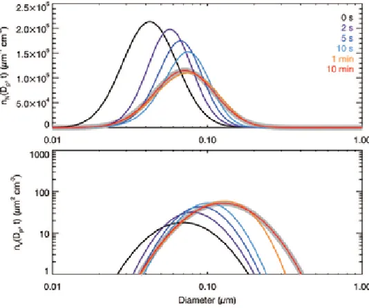
equations (1) and (45) together. Figure 1.3 shows the time evolution of the aerosol with

!! ! !"!!!!"# and !!"!!! ! !"!!!!"#. In the first few minutes, the size distribution

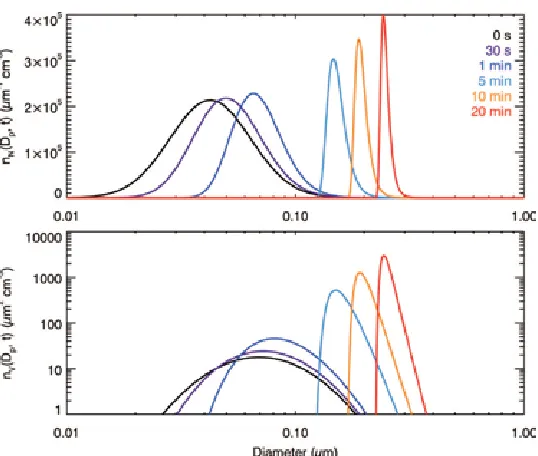
evolves as in diffusion-limited growth, with the width narrowing and the peak increasing with time. After about 10 min, the peak of the size distribution begins to decrease, and the width increases. The retreat of the peak results from the evaporation of small particles as the partial pressure of the ambient gas decreases, while the large particles continue to grow. After 10 hr, the entire system reaches approximately the equilibrium state, which is predicted by the analytical solution (dashed line, equation (1.37)). For a more volatile species with !!"!!! ! !"!!!!"# (Figure 1.4), the system reaches the equilibrium state in

about 10 min.

(36)

[image:36.612.175.436.87.309.2] [image:36.612.173.440.391.614.2]

Figure 1.3. Evolution of the aerosol number distribution, !!!!!! !!, and the volume distribution, !!!!!! !!, in a closed system; !!! !"!!!!"#, !!"!!! ! !"!!!!"#. The gray curve shows the analytical solution for the final distribution (!! ! !!!"#$!!

Figure 1.4. Evolution of the aerosol number distribution, !!!!!!!!, and the volume distribution, !!!!!! !!, in a closed system; !!! !"!!_!!"#_,_!

!"!! ! ! !"!!!!"#. The gray curve shows the

(37)

1.3.3. General System

In the fully general system, there is a constant addition of vapor and at the same time condensation to the particles. One can explore different types of size distribution dynamics by varying the initial distribution (the vapor loss term depends strongly on the total volume

of particles), !, and !!"!!! . In this study, we fix the initial distribution as above and

demonstrate typical evolution patterns. The simulation is based on the simultaneous solution of equations (1.11) and (1.45). Different initial distributions will lead to quantitatively different, but qualitatively consistent, conclusions. For instance, for a larger number concentration (!! is larger), or aerosol volume (!!"is larger), the transition time

from diffusion-limited growth to equilibrium growth will be shorter.

For ! ! !"!!_!!"#!!"#!!_and_!

!"!!! ! !"!!"!!"#! the vapor generation rate is sufficiently

large that vapor loss to particles is relatively unimportant. Figure 1.5 shows the standard diffusion-limited growth pattern that results, as we obtained in the open system (Figure 1).

Again, the inherent growth timescale is governed by !.

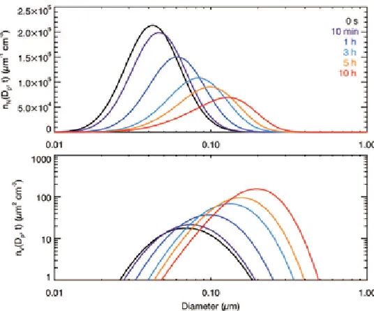
[image:37.612.173.442.419.647.2]

(38)

For ! ! !"!!!_!_!"#_!!"#!!_and_!

!"!!! ! !"!!"!!"#! the vapor generation is sufficiently

slow that the equilibrium partial pressure over the particle surface is able to reach the quasi-equilibrium state, and the size distribution exhibits a shape characteristic of quasi-equilibrium growth (Figure 1.6). Note that the growth in the full system significantly differs from the quasi-equilibrium case in the open system (Figure 1.2). In the quasi-equilibrium case, if the vapor is generated indefinitely, the maximum value of the vapor pressure over the surface of a particle is that of the pure substance, after which a quasi-equilibrium state does not exist. As the particles grow, the capacity to absorb the ambient vapor increases, and the ambient vapor pressure can achieve a nearly constant level when the rate of vapor absorption by the particles equals the rate of vapor generation. Larger particles have a larger absorption capacity so that they grow faster and lead to a broader size distribution.

The growth rate is limited by the rate of change of the ambient partial pressure, !, which

governs the inherent timescale.

Figure 1.6. Simulated evolution of the aerosol number distribution, !!!!!! !! and the volume distribution, !!!!!! !!, in a fully general system;!!!"!! ! ! !"!!"!!"#, ! ! !"!!!!!"#!!"#!!.

In the case of ! ! !"!!_!!"#!!"#!!_and_! !"!!

! _{! !"}!!_!!"#_{, the size evolution pattern}

[image:38.612.172.440.375.598.2]

(39)

minutes, when the vapor partial pressure is not large, the evolution behaves like equilibrium growth; after the gas partial pressure is large enough to maintain the partial pressure gradient, the smaller particles grow faster and catch up with the larger particles, i.e., diffusion-limited growth.

Figure 1.7. Simulated evolution of the aerosol number distribution, !!!!!! !! and the volume distribution, !!!!!! !!, in a fully general system;!!!"!!! !!"!!!!"#, ! !!"!!!!"#!!"#!!.

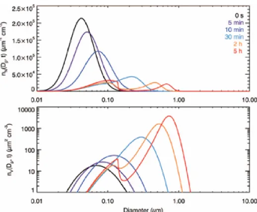
A “two-mode case” is shown in Figure 1.8, with ! ! !"!!_!!"#!!"#!!_and_!

!"!!! !

!"!!_!!"#_{. This case is same as that in Figure 1.7 except that the condensable species is}

more volatile. All the particles grow more slowly because they reach equilibrium more readily. An approximate, but quantitative, explanation may be obtained from equations

(1.31) and (1.32): when ! is larger, !!!! and !!!! are smaller. As the particles grow

larger, the rate of vapor absorption by the particles increases, and it will slightly exceed the rate of vapor generation (in this case, it occurs at about 30 min). After that, the partial pressure of the ambient gas gradually decreases for a long period. Small particles partial

pressure continues to decrease. However, even larger particles, e.g., ! !!!!!!, continue to

grow by diffusion, because the equilibrium vapor pressure over their surface is still low. A

[image:39.612.172.441.185.408.2]

(40)

near !!!!!! from particles that have partially evaporated. This two-mode feature could persist as long as the partial pressure continues to decrease, until the equilibrium vapor pressure over the large end of the spectrum becomes large enough to reduce the rate of vapor absorption below that of the rate of vapor generation. In the case of Figure 1.7, initially the particles grow faster than the case of Figure 1.8, and the ambient vapor pressure actually starts to decrease much earlier (at about 3 min). However, the small size mode is not obvious because only a tiny fraction of the particles in the small end of the spectrum reach the equilibrium state at that time. By noting this, we can suggest conditions for the occurrence of the two-mode size distribution. (1) A condensable species with an intermediate pure component equilibrium pressure. If !!"!!! is too small, the particles will

exhibit diffusion-limited growth. If the species is too volatile, the particles will grow too slowly to suppress the increase of the partial pressure of the ambient vapor, and the size distribution will just behave as an equilibrium growth. (2) Before the rate of vapor absorption by the particles exceeds the rate of vapor generation, there must be sufficient particles in the equilibrium state in order to form a discernible mode. The two-mode pattern could persist for a long period (10 hr or more in the case of Figure 1.8).

1.4. Atmospheric Implications

(41)

Figure 1.8. Simulated evolution of the aerosol number distribution, !!!!!!!! and the volume

[image:41.612.175.434.86.299.2]

(42)

Chapter II

Sulfur Chemistry in the Middle Atmosphere of Venus

†

“In the course of transformation they are produced and extinguished being born and then dying, dying and then being born, in birth after birth, in death after death, the way a torch spun in a circle forms an unbroken wheel of flame.”

_{The Surangama Sutra, Siddhartha Gautama, 563~483 BC}

Summary

Venus Express measurements of the vertical profiles of SO and SO2 in the middle

atmosphere of Venus provide an opportunity to revisit the sulfur chemistry above the Middle cloud tops (~58 km). A one dimensional photochemistry-diffusion model is used to simulate the behavior of the whole chemical system including oxygen-, hydrogen-, chlorine-, sulfur-, and nitrogen-bearing species. A sulfur source is required to explain the

SO2 inversion layer above 80 km. The evaporation of the aerosols composed of sulfuric

acid (model A) or polysulfur (model B) above 90 km could provide the sulfur source.

Measurements of SO3 and SO (!!!! !!!!!) emission at 1.7 µm may be the key to

distinguish between the two models.

2.1. Introduction

Venus is a natural laboratory of sulfur chemistry. Due to the difficulty of observing the lower atmosphere, we are still far from unveiling the chemistry at lower altitudes (Mills et al. 2007). On the other hand, the relative abundance of data above the middle cloud tops (~58 km) allows us to test the sulfur chemistry in the middle atmosphere. Mills et al. (2007)

† Appeared as: Zhang, X., Liang, M.C., Mills, F.P., Belyaev, D., Yung, Y.L., 2012. Sulfur chemistry

(43)

summarized the important observations before Venus Express and gave an extensive review of the sulfur chemistry on Venus.

Recently, measurements of Venus Express and ground-based observations have greatly improved our knowledge of the sulfur chemistry. Marcq et al. (2005; 2006; 2008) reported

the latitudinal distributions of CO, OCS, SO2 and H2O in the 30-40 km region. The

anti-correlation of latitudinal profiles of CO and OCS implies the conversion of OCS to CO in the lower atmosphere (Yung et al. 2009). Using the latitudinal and vertical temperature distribution obtained by Pätzold et al. (2007), Piccialli et al. (2008) deduced the dynamic structure, which shows a weak zonal wind pattern above ~70 km. The discovery of the nightside warm layer by the Spectroscopy for Investigation of Characteristics of the Atmosphere of Venus (SPICAV) onboard Venus Express (Bertaux et al. 2007) is a strong evidence of substantial heating in the lower thermosphere (above 90 km). Near the antisolar point, this heating is consistent with the existence of a subsolar-antisolar (SSAS) circulation. However, the nightside warm layer has been reported in SPICAV observations at all observed local times and latitudes and does not appear to be consistent with ground-based submillimeter observations (Clancy et al. 2008). Through the occultation technique, Solar Occultation at Infrared (SOIR) and SPICAV carry out measurements of the vertical

profiles of major species above 70 km, including H2O, HDO, HCl, HF (Bertaux et al.

2007), CO (Vandaele et al. 2008), SO and SO2 (Belyaev et al. 2008; 2011). Aerosols are

found to be in a bimodal distribution above 70 km (Wilquet et al. 2009). These high vertical resolution profiles are obtained mainly in the polar region. Using the SPICAV

nadir mode, Marcq et al. (2011a) found large temporal and spatial variations of the SO2

column densities above the cloud top in the period of 2006-2007, which suggests that the cloud region is dynamically very active. Ground-based measurements also provide valuable information. Krasnolposky (2010a; 2010b) obtained spatially resolved

distributions of CO2, CO, HDO, HCl, HF, OCS, and SO2 at the cloud tops from the

CSHELL spectrograph at NASA/IRTF. Sandor et al. (2010) reported ground-based

submillimeter observations of SO and SO2 inversion layers above 85 km. The

(44)

Express (Belyaev et al. 2011). However, only the smallest SO and SO2 abundances inferred from the SPICAV observations (Belyaev et al. 2011) are quantitatively similar to those inferred from the submillimeter observations (Sandor et al. 2010). Spatial and temporal variability may explain at least some of the differences among the observations (Sandor et al. 2010), but detailed inter-comparisons are required. These measurements and

the proposed correlation of upper mesosphere SO2 abundances with temperature open up

new opportunities to study the photochemical and transport processes in the middle atmosphere of Venus.

Sandor et al. (2010) found that SO and SO2 inversion layers cannot be reproduced by the

previous photochemical model (Yung and DeMore 1982). Therefore they suggested that

the photolysis of sulfuric acid aerosol might directly produce the gas phase SOx. A detailed

photochemical simulation by Zhang et al. (2010) showed that the evaporation of H2SO4

aerosols with subsequent photolysis of H2SO4 vapor could provide the major sulfur source

in the lower thermosphere if the rate of photolysis of H2SO4 vapor is sufficiently high.

Their models also predicted supersaturation of H2SO4 vapor pressure around 100 km. The

latest SO and SO2 profiles retrieved from the Venus Express measurements agree with their

model results (Belyaev et al. 2011). This mechanism reveals the close connection between the gaseous sulfur chemistry and aerosols. Previously sulfuric acid was considered only as the ultimate sink of gaseous sulfur species in the middle atmosphere. If it could also be a

source, the thermodynamics and microphysical properties of H2SO4 must be examined

more carefully. Alternatively, if the polysulfur (Sx) is indeed a significant component of the

aerosols as the unknown UV absorber, Carlson (2010) estimated that the elemental sulfur is

about 1% of the H2SO4abundance. This might also be enough to produce the sulfur species

if there is a steady supply of Sxaerosols to the upper atmosphere.

(45)

90 km, H2SO4 and Sx, respectively, the roles they play in the sulfur chemistry, their implications and how to distinguish the two sources by the future observations. The last section provides a summary of the chapter and conclusions.

2.2. Model Description

Our photochemistry-diffusion model is based on the one-dimensional Caltech/JPL kinetics code for Venus (Yung and DeMore 1982; Mills 1998) with updated chemical reactions. The model solves the coupled continuity equations with chemical kinetics and diffusion processes, as functions of time and altitude from 58 to 112 km. The atmosphere is assumed to be in hydrostatic equilibrium. We use 32 altitude grids with increments of 0.4 km from 58 to 60 km and 2 km from 60 to 112 km. The diurnally averaged radiation field from 100 to 800 nm is calculated using a modified radiative transfer scheme including gas absorption, Rayleigh scattering by molecules and Mie scattering by aerosols with wavelength-dependent optical properties (see appendix A). The unknown UV absorber is approximated by changing the single scattering albedo of the mode 1 aerosols beyond 310

nm, as suggested by Crisp (1986). Because the SO, SO2 and aerosol profiles from Venus

Express are observed in the polar region during the solar minimum period (2007-2008), our

calculations are set at a circumpolar latitude (70°N) and we use the low solar activity solar

spectra for the duration of the Spacelab 3 ATMOS experiment with an overlay of Lyman alpha as measured by the Solar Mesospheric Explorer (SME).

In this study we selected 51 species, namely, O, O(1_{D), O}

2, O2(1$), O3, H, H2, OH, HO2, H2O, H2O2, N2, Cl, Cl2, ClO, HCl, HOCl, ClCO, COCl2, ClC(O)OO, CO, CO2, S, S2, S3, S4, S5, S7, S8, SO, (SO)2, SO2, SO3, S2O, HSO3, H2SO4, OCS, OSCl, ClSO2, four

chlorosulfanes (ClS, ClS2, Cl2S, and Cl2S2) and eight nitrogen-containing species (N, NO,

NO2, NO3, N2O, HNO, HNO2, and HNO3). The chlorosulfanes (SmCln) are included

because they open an important pathway to form S2and polysulfur Sx(x=2%8) in the region

(46)

because the SmCln abundances are low. Nitrogen-containing species, especially NO and

NO2, can act as catalysts for converting SO to SO2and O to O2in the 70~80 km region

(Krasnopolsky 2006). A recent study by Sundaram et al. (2011) suggests that the odd

nitrogen (NOx) chemistry might also have significant effects on the abundances of sulfur

oxides in the 80~90 km region.

In Zhang et al. (2010), the chemistry was simplified because (SO)2, S2O and HSO3were

considered only as the sinks of the sulfur species. This might not be accurate enough for the

chemistry below 80 km where there seems to be difficulty in matching the SO2

observations. Instead, a full set of 41 photodissociation reactions is used here, along with about 300 neutral chemical reactions, as listed in appendix A. We take the ClCO thermal

equilibrium constant from the 1-! model in Mills et al. (2007) so that we can constrain the

total O2column abundances to ~2&1018 cm-2. In addition, we introduce the heterogeneous

nucleation processes of elemental sulfur (S, S2and polysulfur) because these sulfur species

can readily stick to sulfuric acid droplets and may provide the source material for the unknown UV absorber (Carlson 2010). But we neglect all the heterogeneous reactions among the condensed elemental sulfur species on the droplet surface. The calculation of the heterogeneous condensation rates is described in appendix A. The accommodation coefficient " is varied from 0.01 to 1 for the sensitivity study (section 2.4).

The temperature profiles are shown in Figure 2.1 (left panel). The daytime temperature profile below 100 km (solid line) is obtained from the observations of VeRa onboard

Venus Express near the polar region (71°N, figure 1 of Pätzold et al. 2007). Above 100 km

the temperature is from Seiff (1983). The nighttime temperature profile (dashed line) above 90 km is measured by Venus Express in orbit 104 at latitude 4° S and local time 23:20 h (black curve in the figure 1 of Bertaux et al. 2007). The nighttime temperature profile is

(47)

Figure 2.1. Left panel: daytime temperature profile (solid) and nighttime temperature profile (dashed). Right panel: eddy diffusivity profile (solid) and total number density profile (dashed).

In the 1-D model, species are assumed to be mixed vertically by turbulent eddies. Molecular diffusion becomes important above the homopause region (130~135 km). The eddy diffusivity increases with altitude in the Venus mesosphere for reasons discussed later. Since the zonal wind is observed to decrease with altitude above 70 km due to the temperature gradient from pole to equator (Piccialli et al. 2008), we assume that vertical transport of gas species is predominantly due to mixing caused by transient internal gravity waves, as proposed by Prinn (1975). In this case the eddy diffusion coefficient will be inversely proportional to the square root of the number density (Lindzen 1981). Von Zahn et al. (1979) derived the eddy diffusion coefficient ~1.4&1013 [M]-0.5 cm2 s-1 from the number density around the homopause region, based on mass spectrometer measurements from Pioneer Venus. We use slightly larger values Kz = 2.0&1013 [M]-0.5 cm2 s-1 above 80 km to include an additional contribution of the SSAS circulation. In the region below 80

km, Woo and Ishmaru (1981) estimated the diffusivity # 4.0&104_cm2 _s-1_{at ~60 km from}

radio signal scintillations. Therefore our eddy diffusivity profile from 58~80 km is estimated by linear interpolation between the values at 80 and 60 km. The eddy diffusion profile is shown in Figure 2.1 (right panel). However, the vertical advection due to the SSAS circulation might be dominant above 90 km. The SPICAV measurements show that

150 200 250 Temperature (K) 60

70 80 90 100 110

Altitude (km)

102 ₁₀4 ₁₀6 Eddy Diffusivity (cm2_s-1₎

60 70 80 90 100 110 1014 Number Density (cm₁₀16 ₁₀18

(48)

the SO2 mixing ratio from ~90-100 km is almost constant with altitude, which implies a very efficient transport process.

Since Zhang et al. (2010) has already shown that the model without additional sulfur

sources above 90 km cannot explain the observed SO2 inversion layer, we focus on two

models in this study: model A with enhanced H2SO4 abundance above 90 km and model B

with enhanced S8 abundance above 90 km. In both models we fix the vertical profiles of

N2, H2O, and H2SO4. The N2 profile is given by a constant mixing ratio of 3.5%. The H2O

profile (see Figure 2.3) is prescribed on the basis of the Venus Express observations (Bertaux et al. 2007) above 70 km and is assumed to be constant below. The accommodation coefficient of the sulfur nucleation is set to unity (the upper limit) in the standard model.

The H2SO4saturation vapor pressure (SVP) and the photolysis cross sections are discussed

in appendix A. appendix A also shows that the H2SO4 weight percent profile derived from

thermodynamics under the conditions of the Venus mesosphere is consistent with the

photometric observations. Model A uses the nighttime H2SO4 vapor abundance (Figure

A.6) and the H2SO4photolysis cross sections with high UV cross section in the interval

195-330 nm (dashed line in Figure A.7). The H2SO4 abundance above 90 km is scaled to

reproduce the observed SO and SO2 data. The day and nighttime Sxsaturated mixing ratio

profiles based on Lyons (2008) are shown in Figure A.6. The S8 mixing ratio under

nighttime temperature could achieve ppb levels at ~96 km. Based on this, we fix the S8

profile in model B as the sulfur source. The S8 profile is composed of two parts: (1) below

90 km, we use the output from model A, which shows the S8 concentration is

undersaturated; (2) above 90 km, we scale the S8 saturated vapor abundances under

nighttime temperature to match the observations. We also adopt the daytime H2SO4vapor

abundance and the H2SO4 photolysis cross sections with low UV cross section in the

interval 195-330 nm (solid line in Figure A.7); therefore the H2SO4 photolysis has almost

Aerosols and Chemistry in the Planetary Atmospheres