The GALAH survey: second data release

The GALAH Survey: second data release

Sven Buder,

Martin Asplund,

Ly Duong,

Janez Kos,

Karin Lind,

Melissa K. Ness,

Sanjib Sharma,

Joss Bland-Hawthorn,

Andrew R. Casey,

Gayandhi M. De Silva,

Valentina D’Orazi,

Ken C. Freeman,

Geraint F. Lewis,

Jane Lin,

Sarah L. Martell,

Katharine J. Schlesinger,

Jeffrey D. Simpson,

Daniel B. Zucker,

Tomaˇz Zwitter,

Anish M. Amarsi,

Borja Anguiano,

Daniela Carollo,

Luca Casagrande,

Klemen ˇ

Cotar,

Peter L. Cottrell,

Gary Da Costa,

Xudong D. Gao,

Michael R. Hayden,

Jonathan Horner,

Michael J. Ireland,

Prajwal R. Kafle,

Ulisse Munari,

David M. Nataf,

Thomas Nordlander,

Dennis Stello,

Yuan-Sen Ting (

),

Gregor Traven,

Fred Watson,

Robert A. Wittenmyer,

Rosemary F. G. Wyse,

David Yong,

Joel C. Zinn,

Maruˇsa ˇ

Zerjal

and the GALAH collaboration

Affiliations are listed at the end of the paper

Accepted 2018 April 28. Received 2018 April 17

A B S T R A C T

The Galactic Archaeology with HERMES (GALAH) survey is a large-scale stellar spectro-scopic survey of the Milky Way, designed to deliver complementary chemical information to a large number of stars covered by theGaiamission. We present the GALAH second public data release (GALAH DR2) containing 342 682 stars. For these stars, the GALAH collaboration provides stellar parameters and abundances for up to 23 elements to the community. Here we present the target selection, observation, data reduction, and detailed explanation of how the spectra were analysed to estimate stellar parameters and element abundances. For the stellar analysis, we have used a multistep approach. We use the physics-driven spectrum synthesis of Spectroscopy Made Easy(SME) to derive stellar labels (Teff, logg, [Fe/H], [X/Fe],vmic,vsini, AKS) for a representative training set of stars. This information is then propagated to the whole sample with the data-driven method ofThe Cannon. Special care has been exercised in the spectral synthesis to only consider spectral lines that have reliable atomic input data and are little affected by blending lines. Departures from local thermodynamic equilibrium (LTE) are considered for several key elements, including Li, O, Na, Mg, Al, Si, and Fe, using 1DMARCS

stellar atmosphere models. Validation tests including repeat observations, Gaiabenchmark stars, open and globular clusters, and K2 asteroseismic targets lend confidence to our methods and results. Combining the GALAH DR2 catalogue with the kinematic information from Gaiawill enable a wide range of Galactic Archaeology studies, with unprecedented detail, dimensionality, and scope.

Key words: Surveys – the Galaxy – methods: observational – methods: data analysis – stars: fundamental parameters – stars: abundances.

_{E-mail:[email protected]}

1 I N T R O D U C T I O N

The last decade has seen a revolution in Galactic astronomy. This is particularly evident in the domain of spectroscopic studies where sample sizes have grown from tens or hundreds of stars to several hundred thousands of stars, enabled by the availability of

2018 The Author(s)

object spectrographs. We now live in an extraordinary era of inter-est and invinter-estment in stellar surveys of the Milky Way. At optical and infrared wavelengths, large-scale photometric surveys have de-livered accurate photometric magnitudes and colours for several

hundred millions of stars (e.g. Skrutskie et al.2006; Saito et al.

2012; Chambers et al.2016; Wolf et al.2018).

Spectroscopic surveys of stars in our Galaxy are fundamental to astrophysics because there are important measurements that can only be made in the near-field and through stellar spectroscopy. This is especially true for the measurement of detailed chemical compo-sitions of stars. The determination of accurate stellar ages continues to be a challenge but there is cautious optimism that the situation will improve in the decades ahead. Asteroseismic surveys from

NASA’sKeplerand K2 missions are providing reliable estimates of

stellar surface gravities and masses (e.g. Stello et al.2015; Sharma

et al.2016) and this is expected to continue with missions like TESS

(Ricker et al.2015; Sharma et al.2018) and PLATO (Rauer et al.

2014; Miglio et al.2017). The ESAGaiaastrometric mission will

measure accurate distances for billions of stars belonging to most

components of the Galaxy (Perryman et al.2001; Lindegren et al.

2016).

The Galactic Archaeology with HERMES (GALAH) survey1

brings a unique perspective to the outstanding problem of

under-standing the Galaxy’s history (De Silva et al.2015; Martell et al.

2017). Our study makes use of the High Efficiency and Resolution

Multi-Element Spectrograph (HERMES) at the Anglo-Australian

Telescope (Barden et al.2010; Sheinis et al.2015). This unique

instrument employs the Two Degree Field (2dF) fibre positioner on

the Anglo-Australian Telescope to provide multiobject (n∼392),

high-resolution (R∼28 000) spectra optimized for elemental

abun-dance studies for up to 30 elements in four optical windows. The HERMES instrument was built specifically for the GALAH survey and is largely achieving its original design goals, as we demonstrate here in our major data release (DR2).

The overarching goal of the GALAH survey is to acquire high-resolution spectra of a million stars for chemical tagging, in or-der to investigate the assembly history of the Galaxy (Freeman

& Bland-Hawthorn2002; De Silva, Freeman & Bland-Hawthorn

2009; Bland-Hawthorn, Krumholz & Freeman2010). The GALAH

selection criteria are simple, with the baseline selection being a

magnitude cut of 12<V<14 with Galactic latitude|b|>10 deg.

As such, GALAH probes mainly FGK stars of the thin and thick disc of the Galaxy. However, due to the unprecedented sample size, the survey also includes a substantial number of halo stars, as well as other stellar populations serendipitously along the GALAH stars the line of sight, such as stars in the Magellanic clouds. In addition, complementary programs with the same instrument targeting the Milky Way bulge (Duong et al., in preparation) and open clusters (De Silva et al., in preparation) are under way. For the main GALAH survey, roughly two-thirds of the sample are dwarf stars, whilst the rest are predominantly red giant branch stars located at distances up to several kpc from the solar neighbourhood.

Whilst the volume and wealth of detail contained within the GALAH data set present a broad range of science opportunities in Galactic and stellar astrophysics, such work is beyond the scope of this publication. The key science questions that motivated the GALAH survey are as follows:

(i) What were the conditions of star formation during early stages of Galaxy assembly?

1_{https://galah-survey.org/}

(ii) When and where were the major episodes of star formation in the disc, and what drove them?

(iii) To what extent are the Galactic thin and thick discs composed of stars from merger events?

(iv) Under what conditions and in what types of systems did accreted stars form?

(v) How have the stars that formedin situin the disc evolved

dynamically since their formation?

(vi) Where are the solar siblings that formed together with our Sun?

The above science questions can be presented as specific delivery goals for the survey. It is these delivery goals that are the highlight of this Data Release. The goals can be summarized as follows:

(i) To determine the primary stellar parameters: effective tem-perature, surface gravity, metallicity

(ii) To derive up to 30 individual chemical element abundances per star from Li to Eu

(iii) To measure radial velocities

(iv) To classify targets of an ‘unusual’ nature: e.g. binaries, stellar activity, chemical peculiarities

Achieving the above delivery goals for millions of stars in an unrestricted parameter space is a major challenge; doing so con-sistently and in a timely manner takes us into new territory for spectral analysis methods. Teams have been required to revisit their classical approach and enter into other disciplines of data analysis to develop machinery suitable for meeting these new challenges. In recent years, we have learned to bring together many different

strands to make progress (Ho et al.2017). This has required major

advances in a range of areas, including template matching (Jofr´e

et al. 2010), automated machine learning (Ness et al.2015),

at-mospheric modelling (Magic et al.2013), spectral line formation

(Amarsi et al.2016a), and internal instrument calibrations

(Bland-Hawthorn et al.2017; Kos et al.2018b). We discuss some of these

advances to the extent that they have benefited the GALAH data reduction and analysis, as part of this paper.

The GALAH survey joins a vibrant and exciting landscape of Galactic spectroscopic surveys that are highly complementary in

scale and scope. TheGaia-ESO Survey on the VLT (Gilmore et al.

2012; Randich et al.2013) contains a sample of about 100 000 stars

over 14–19 inVband, most of which are thick disc and halo stars,

as well as numerous open clusters. The observations used specific spectral windows with the GIRAFFE+FLAMES fibre spectrograph

system, and the typical spectral resolving power isR ≈ 20 000,

somewhat lower than that of GALAH. However, a subsample of targets observed with the UVES spectrograph have high-resolution

(R ≈ 47 000) spectra. The infrared APOGEE survey (Abolfathi

et al.2018) mainly targets the low-latitude Galactic disc, probing

through the optically thick dust regions with a sample of 150 000 red

giants at a resolving power ofR≈22 500. To expand their survey,

the APOGEE team has recently begun the APOGEE-South survey, using the Dupont telescope at Las Campanas Observatory, in order to study a similar number of stars in the southern sky. While the overlap in targets between the three surveys is currently only a few hundred stars, the scientific complementarity is significant. Given the different magnitude ranges and regions of the Galaxy observed,

both Gaia-ESO and APOGEE are highly complementary to the

GALAH sample. Several even larger high-resolution spectroscopic surveys of the Milky Way are expected to commence over the next

decade, including WEAVE (Dalton et al.2014), 4MOST (de Jong

et al.2014), and SDSS5 (Kollmeier et al.2017).

LAMOST is a lower spectral resolution (R∼1800) survey but has observed a far greater number of stars than other surveys, with

over 1.5 million stellar spectra collected to date (Luo et al.2015).

The RAVE survey (Kunder et al.2017) contains a similar number of

stars as the current GALAH sample but at a lower resolving power of

R=7500 and with the wavelength coverage limited to the infrared

calcium triplet region. The RAVE sample, spanning magnitudes

from 9 to 12 in theI band, was selected from numerous sources

(Tycho-2, super-COSMOS, DENIS, and 2MASS) and included a

colour selection ofJ−K> 0.5 mag for stars with|b|<25◦to

preferentially select giants (see Wojno et al. 2017). The simple

selection function of the GALAH sample, on the other hand, is dominated by local disc dwarfs, making it more sensitive to local

substructure. As part of the secondGaiadata release in 2018 April,

radial velocities for some seven million stars brighter thanG≈

13 have been measured based onR=11 500 spectra around the

Ca infrared triplet (845–872 nm) that also provide information on stellar parameters and some limited elemental abundances.

In this paper, we present the second major public data release of the GALAH survey including stellar parameters and individual abundances of 23 elements from Li to Eu for 342 682 stars. In Sec-tion 2 we provide an overview of the target selecSec-tion, observaSec-tion, and reduction procedures. In Section 3 we present the details of the spectroscopic analysis, followed by a description of the validation in Section 4 and contents of the data release in Section 5. We high-light studies of the GALAH team accompanying these data release in Section 6before we conclude in Section 7.

2 TA R G E T S E L E C T I O N , O B S E RVAT I O N , R E D U C T I O N

2.1 Target selection

In order to carry out a large-scale survey with broad applications across astrophysics and Galactic archaeology, the GALAH survey uses a very simple observational selection function. This makes it relatively straightforward to transform between the observed data set and the underlying Galactic populations. It also makes a clear imprint on which types of stars across which regions of the Milky Way are sampled by GALAH because of their luminosities.

The GALAH input catalogue is constructed from the union

of 2MASS (Skrutskie et al. 2006) and UCAC4 (Zacharias et al.

2013) catalogues. Only stars with appropriate 2MASS quality flags

(Q=‘A’,B=‘1’,C=‘0’,X=‘0’, A=‘0’, prox≥6) and having no

bright neighbours closer than (130−[10×V]) arcseconds of the

bright starsV magnitude were chosen. Because APASS was not

complete in the Southern sky at the start of observations, we use

a syntheticVJK magnitude calculated from 2MASS photometry:

VJK=K+ 2(J−K+ 0.14) + 0.382e((J−K−0.2)/0.5)_{. Using PARSEC}

isochrones (Marigo et al.2017), it was shown in Sharma et al. (2018)

that this transformation is reasonably accurate across the parame-ter space where the majority of GALAH stars fall. The GALAH observations are done in following three fixed magnitude ranges of VJK.

(i) Normal mode 12<VJK <14: Most observations are done

with this selection function.

(ii) Bright mode 9<VJK<12: This is used during twilight or

poor observing conditions.

(iii) Faint mode 12<VJK<14.3: This is used when fields with

normal or bright configuration are not available to be observed.

As a result of this simple selection function, all stars with−80◦

≤δ≤+10◦and b >10◦within these magnitude limits are

poten-tially targets for our survey. We imposed an additional requirement, namely that we only sample fields with an on-sky density of stars of

at least 400 perπsquare degrees, to match the number of fibres and

field of view of the fibre positioner that feeds our spectrograph. The potential targets are then tiled into 6546 normal fields. The radius of each field varies inversely with the target density, to improve efficiency in dense regions. A normal field can be observed in either normal or bright mode but not faint mode. In bright configuration, the radius is set to 1 deg. In addition to normal fields, 285 faint fields were added to be observed exclusively in faint mode, and they do not overlap with the normal fields.

2.2 Observations

Data for the GALAH survey are taken with the HERMES spec-trograph on the 3.9-metre Anglo-Australian Telescope (AAT) at Siding Spring Observatory. HERMES is a fibre-fed high-resolution

(R= 28 000) spectrograph optimized to do Galactic archaeology

from a 4m class telescope, with four discrete optical wavelength channels covering 4713–4903 Å, 5648–5873 Å, 6478–6737 Å, and

7585–7887 Å (De Silva et al.2015; Sheinis et al.2015).

The 2dF top end for the AAT provides the fibre feed for HERMES

(Lewis et al.2002); its name derives from the 2-deg diameter field

of view. It has two metal field plates, each with 392 science fibres and 8 guide bundles. The fibres are affixed to magnetic ‘buttons’ and placed on the field plate by a robotic fibre positioning system. While one field plate is being observed, the other is in position for set-up by the positioning robot. The 2dF fibres are fed through the telescope structure to the HERMES enclosure on the fourth floor of the AAT dome, where they are arranged into two pseudoslits, such that the set of fibres corresponding to the field plate that is currently being observed is fed into the spectrograph. Light from the fibres is collimated and then sent through a series of dichroic elements to separate the four wavelength channels. It is then dispersed us-ing volume phase holographic diffraction gratus-ings and imaged by four independently controlled cameras. Further details of instru-ment design, and its as-built performance, can be found in Barden

et al. (2010), Brzeski, Case & Gers (2011), Heijmans et al. (2012),

Farrell et al. (2014), and Sheinis et al. (2015).

The GALAH survey observations are carried out by team mem-bers, either at the AAT or from remote observing sites in Australia. TheOBSMANAGERsoftware developed by the team is used to select

a field that will be near the meridian at the time of observation. This field is required to be at least 30 deg from the Moon, to have a relatively small change in airmass over the exposure time, and to have no Solar System planets within it at the time of observation (as bright sources such as Jupiter have caused trouble with scattered light contaminating spectra in previous 2dF survey observations, though HERMES has been found to suffer much less from this than

AAOmega; see Simpson et al.2017). Fiducial targets, used for field

acquisition and guiding, are chosen from the stars with 11≤V≤12

in the input catalogue that are located in the field. For observations

in bright mode fiducial are selected from stars with 12≤V≤13.

Once the observer chooses a field from the options provided byOB

-SMANAGER, it generates a list of targets in the correct input format for

theCONFIGUREsoftware (Miszalski et al.2006), and it tracks which fields have been observed.

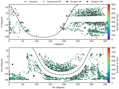
Fig. 1shows maps of GALAH DR2 stars (observed between

2014 January 16 and 2018 January 29) in equatorial and Galactic coordinates. The target selection can clearly be seen in the avoidance

Figure 1. Distribution of observed fields in Galactic and Equatorial coordinates. The fields are color coded by the number of observed stars. The bold dashed line corresponds to equatorial (upper panel) and Galactic (lower panel) equators. The equatorial, the ecliptic, and the Galactic south poles are also marked as black symbols on the panels.

of the Galactic plane and of fields at high Galactic latitude where

the target density is too low. Fig.2shows the distribution ofVJKin

DR2. The upper panel shows the overall distribution and subdivides the data into bright, regular, and faint survey fields, and the lower panel is a cumulative histogram.

CONFIGUREuses a simulated annealing algorithm to identify a set

of target allocations for the 2dF fibres that maximizes the number of science targets observed and the number of fiducial targets used for field alignment and guiding. It then places a user-defined number of fibres on sky locations, follows user-defined target priorities, and obeys restrictions on fibre placement (as an example, because of the size of the 2dF buttons, the minimum fibre spacing is 30 arcsec, although the fibres themselves have a field of view of only 2 arcsec).

The output ofCONFIGUREis then passed to the 2dF fibre positioning

robot, which places the fibres serially onto the currently unused field plate, checking that each is within an acceptable tolerance of its intended position. Field set-up typically takes 40 min for a full 400-target field, and essentially no survey observing time is lost

waiting for reconfiguration. As discussed in Martell et al. (2017),

the exposure time is set to achieve a signal-to-noise ratio (SNR) of 100 per resolution element, at an apparent magnitude of 14 in the Johnson/Cousins filter closest to each bandpass. For regular survey fields, the standard procedure is to take three 1200-s exposures. If the seeing is between 2 and 2.5 arcsec, this is extended to four exposures, and to six exposures, if the seeing is between 2.5 and

Figure 2. Distribution ofV- band magnitude of GALAH stars. The distri-butions for normal, bright, and faint fields are shown separately.

Figure 3. Distribution of SNR per pixel for the different HERMES wave-length bands. The numbers in the upper left corner denote the 16th, 50th, and 84th percentile values.

3 arcsec. For bright fields, three 360 s exposures are taken. Fig.3

shows cumulative distributions for SNRper pixelin each of the four

HERMES channels. With about four pixels per resolution element, the SNR per resolution element is almost twice what is shown in

Fig.3.

Fibre flat fields and ThXe arc exposures, both with exposure times of 180s, are taken along with each science field. Including the readout time of 71 s and a slew and acquisition time of 2–5 min per field, the time spent on overheads is roughly 20 per cent of the time spent acquiring science data. The typical data rate in survey fields is 4.2 stars per on-sky minute. The GALAH survey has typically been awarded 35 nights per semester since 2014 February, secured across a number of competitive time-allocation rounds.

2.3 Data reduction

We use a reduction pipeline designed specifically for the GALAH survey, where steps are tailored to the observing strategy and scien-tific requirements of the survey. The reduction pipeline is described

in detail in a separate paper (Kos et al.2017) with only a short

overview given here.

Raw images are corrected for the bias level using a series of bias frames taken every night. One flat field exposure is taken for each science field, which is used to identify damaged columns and pixels, serves as a reference to find spectral traces on the science images, and supports the measurement of scattered light and fibre cross-talk.

After cosmetic corrections, the cosmic rays are removed utilizing

a modified LaCosmic algorithm (Van Dokkum2001). Before the

extraction of the spectra, a geometric transformation is used to correct some basic optical aberrations. This reduces the variation of resolving power between different fibres and different wavelength regions.

To ensure the most accurate analysis of our data, we have refined the previously measured literature wavelengths for the ThXe arc lamp. The wavelength fitting algorithm has been improved since

the publication of Kos et al. (2017), so it now learns the trends

and instabilities in the wavelength calibration to predict a better solution when arc lamp spectra are hard to identify. We have to rely on weak lines in the ThXe arc lamp spectrum to calibrate the wavelengths. These are hard to measure in low throughput fibres, so the wavelength calibration for some fibres and some wavelength regions was suboptimal in previous reductions.

The sky spectrum is modelled from ∼25 dedicated sky fibres

over the whole 2◦focal plane. After the sky spectrum is subtracted,

a telluric absorption spectrum is calculated usingMOLECFITsoftware

(Kausch et al.2015; Smette et al.2015) and the science spectra are

corrected.

The products of the reduction pipeline are unnormalized and normalized spectra, together with an uncertainty spectrum and a resolution map.

At the end of the reduction pipeline we calculate basic stellar

parameters for all reduced objects. Radial velocitiesrv syntand

their errorse rv syntare computed by cross-correlating reduced

spectra with 15 synthetic AMBRE spectra (De Laverny et al.2012).

Barycentric corrections are applied to the spectra (Kos et al.2017).

Barycentric radial velocities are measured independently in the blue, green, and red channels, which are weighted to yield one radial ve-locity with its uncertainty. Such radial velocities are precise enough for most of the following analysis. First they are used for a con-tinuum normalization calculated from regions minimally affected by spectral lines. Normalized spectra are then shifted to rest-frame wavelength and matched with 16 783 synthetic AMBRE spectra to

estimate initial values of effective temperatureTeff, surface gravity

logg, and metallicity [M/H] for the subsequent detailed spectral

analysis.

2.4 Alternative radial velocities

The high SNR and resolution of HERMES spectra with a wide wavelength coverage and careful data reduction make GALAH an

excellent source of accurate radial velocities in the 12<V<14

magnitude range to complement, e.g. Gaiadistances and proper

motions. To achieve this goal, we measure radial velocities in a

custom three-stage process (Zwitter et al.2018). First, we build a

library of median observed spectra with very similar stellar param-eter values. In particular, we combine spectra within bins of 50 K

inTeff, 0.2 dex in loggand 0.1 dex in [Fe/H]. Initial values of radial

velocities, as measured by the data reduction pipeline, allow us to perform this task with virtually no velocity smearing. These me-dian spectra have a very high SNR and are used in the second stage to measure the radial velocity of an observed spectrum versus its corresponding median spectrum very accurately. At this stage, the median spectrum is not guaranteed to be at zero velocity due to the combined effects of convective line shifts and gravitational redshifts

(Asplund et al.2000; Allende Prieto et al.2013). We therefore use

the grid of synthetic spectra (Chiavassa et al.2018) computed with

3D hydrodynamical stellar atmosphere models with the STAGGER

code (Magic et al.2013), which include the effects of convective

motions in stellar atmospheres. Finally, we incorporate the effects of gravitational redshift, to put spectra of different stellar types on the same scale and thus allows us to speak about the accuracy and not just the precision of radial velocities. This can be crucial when studying the internal dynamics of stellar clusters, associations, or streams, which generally contain different types of stars and in

which relative velocities do not exceed a few km s−1_.

The propagation of internal velocity errors, as well as the com-parison of velocities measured for multiple observations of the same object, shows that a typical error of derived radial velocities is close

to 0.1 km s−1_{. It can be worse for turn-off stars where accurate}

radii and masses of stars are unknown, so that reliable values of gravitational redshift cannot be determined. Our velocity results are

reported in three columns:rv obstis the final value of the radial

velocity, including the gravitational redshift,e rv obstis its

for-mal error, andrv nogr obstis the value of the radial velocity

without gravitational redshift. The latter may be useful for two pur-poses: (i) to compare our results to those of other surveys, which generally do not take gravitational redshift into account, and (ii)

to allow the user to use a different, more accurate value of

gravita-tional redshift. In particular, astrometric results fromGaiaDR2 will

allow an accurate estimate of the absolute magnitude of the source

which, when combined with the value ofTeffwe report here, will

al-low the accurate calculation of the stellar radius. However this will require an estimate of extinction; we discuss prospects for measur-ing extinction below. Once the radius is estimated, isochrones and metallicities can be used to estimate the object’s mass, and hence to determine the value of gravitational redshift. Details of the above procedure and comparison to results of other radial velocity surveys

are discussed in more detail elsewhere (Zwitter et al.2018).

3 A N A LY S I S

In this section, we describe the multistep approach we use to es-timate stellar parameters and element abundances from GALAH spectra.

3.1 Analysis strategy

Because of the large volume of data, we are using a new data analy-sis approach, which has proven successful when dealing with very large data sets: train a data-driven approach on physics-driven input to connect data (spectra) with labels (in our case stellar parameters and element abundances) and then propagate this information onto the whole sample. We first create such a training set of 10 605 stars and estimate stellar labels through detailed spectrum synthesis using the code Spectroscopy Made Easy (Section 3.2), investing much effort ensuring that the inferred stellar parameters and abun-dances are trustworthy [e.g. line selection, atomic/molecular data, blends, non-local thermodynamic equilibrium (LTE) effects]. We

then create spectral models withThe Cannonand use these models

to propagate the information from the training set on to the whole survey (Section 3.3). This approach makes the implementation of

a flagging algorithm vital, becauseThe Cannonin its current form

will always produce label estimates, which then have to be vetted as we describe in Section 3.4.

3.2 Analysis step 1: the training set analysis withSpectroscopy Made Easy

For the model-driven analysis, we use the spectral synthesis code

SME (Spectroscopy Made Easy) v360 (Valenti & Piskunov1996;

Piskunov & Valenti2017). SME performs spectrum synthesis for

1D stellar atmosphere models, which in our case for DR2 consist of

MARCStheoretical 1D hydrostatic models (Gustafsson et al.2008);

we use spherical symmetric stellar atmosphere models for logg≤

3.5 assuming 1Mand plane-parallel models otherwise. While the

radiative transfer in SME is typically carried out under the assump-tion of LTE, it is possible to provide departure coefficients for level populations calculated elsewhere; we make use of this feature in the GALAH survey in order to derive accurate stellar parameters and elemental abundances as free of systematic errors as possible. For DR2 we incorporate non-LTE line formation for several key

el-ements, including Li (Lind, Asplund & Barklem2009), O (Amarsi

et al.2016a), Na (Lind et al.2011), Mg (Osorio et al.2015), Al

(Nordlander & Lind2017), Si (Amarsi & Asplund2017), and Fe

(Amarsi et al.2016b), mostly with additional dedicated calculations

in addition to those previously published. In all cases the non-LTE computations have been performed using exactly the same grid of 1DMARCSmodel atmospheres. Future GALAH data releases will

have additional elements treated in non-LTE.

In addition to providing a formal solution of the radiative trans-fer, SME attempts to find the optimal solution for various free parameters specified by the user; we use this feature to estimate

the stellar parameters of the GALAH targets, allowingTeff, logg,

[Fe/H], [X/H],Vbroad(spectral line broadening, consisting of the

combined effects of macroturbulence and rotation),vradand

contin-uum normalization to vary during the optimization process. We have carefully selected the most reliable atomic lines within the HERMES wavelength regions to ensure accurate determination of the stellar parameter and abundances for the analysis of late-type stars. The line-list selection was originally done in conjunction with

the corresponding compilation for the Gaia-ESO survey (Heiter

et al.2015a). Our guiding principle has been to include only

spec-tral lines that both have reliable atomic data and be as little affected by blending lines as possible. Naturally this dramatically limits the number of spectral features to be used in late-type stellar spectra, since the majority of lines are either blended to various extent and/or lack good atomic data, especially transition probabilities. The selec-tion of lines to employ was initially based on a detailed comparison of the predicted spectrum against observations for the Sun and Arc-turus but also tested for other benchmark stars. Whenever possible, experimental oscillator strengths are used if trustworthy, but for some lines used as elemental abundance diagnostics we have had to resort to more or less uncertain theoretical transitional probabil-ities in the absence of better alternatives. Astrophysical calibration

offvalues was not performed. In addition to the primary line list

for abundance purposes, we have included background blending

lines, which have largely been taken from theGaia-ESO linelist; in

several cases we have updated the oscillator strengths (loggf)

em-pirically compared to those in theGaia-ESO master linelist in order

to provide better agreements between observed HERMES spectra and the predicted stellar spectrum for stars. The list of the primary spectral lines used for the determination of stellar parameters and

abundances is given in TableA1.

To determine stellar parameters, we make use of theTeff-sensitive

Hαand Hβlines (e.g. Amarsi et al.2018) and neutral/ionized lines

of Sc, Ti, and Fe; the latter elements provide constraints on the

ef-fective temperature and surface gravity loggthrough excitation and

ionization balance as well as metallicity. SME first synthesizes the initial model based on radial velocities from the reduction process and a set of initial stellar parameters. If available and not flagged,

stellar parameters from a prior version ofThe Cannon(version 1.3)

are chosen. This version was also used for previous data releases

of GALAH (Martell et al.2017), TESS-HERMES (Sharma et al.

2018), and K2-HERMES (Wittenmyer et al.2018). If these

param-eters are flagged or not available, the synthesis commences with the stellar parameter estimates from the reduction process. If these are also flagged, we start from an arbitrary set of stellar parameters

(Teff=5000 K, logg=3.5 dex, and [M/H]= −0.5 dex).

We then use two main iteration cycles in SME to optimize the parameters, unless we have to use the arbitrary set of stellar param-eters, in which case the second iteration cycle is repeated. In the first cycle, each wavelength segment of typically 10 Å is normal-ized using a linear function, which is adequate for the short wave-length intervals used here. SME then computes synthetic spectra

in 46 selected (masked) regions. The free parameters Teff, logg,

[M/H],2 _ξ

t (micro turbulence), vsini(rotational velocity)m, and

radial velocity (vrad) are simultaneously determined. SME uses the

2_{SME returns the iron abundance of the of the best-fit model atmosphere} and spectrum during the parameter determination stage, which is called metallicity, or [M/H].

Levenberg–Marquardt algorithm to find parameters that correspond

to the near-minimumχ2_.

The final parameters from the first cycle are used to synthesize the initial model in the second cycle and re-normalize each seg-ment. SME goes through the same iteration process, optimizing

χ2_{until convergence is achieved (whenχ}2_{changes by less than}

0.1 per cent). The number of iterations necessary to reach conver-gence varies from star to star. Typically, more metal-rich and cooler stars take longer to converge, but normally still do so in fewer than 20 iterations. During the parameter determination, we implement

non-LTE departure coefficients from Amarsi et al. (2016b) for Fe

lines.

While the nominal resolving power of HERMES isR≈28 000, it

is known to vary from fibre to fibre, and as a function of wavelength

(Kos et al.2017). This issue is resolved by interpolating the observed

spectrum with pre-computed resolution maps from Kos et al. (2017)

to estimate a median resolution for each segment. The GALAH survey is currently implementing a photonic comb, which will map the aberrations and point spread function across the full CCD images

(Bland-Hawthorn et al.2017).

3.2.1 Constraints on spectral line broadening

The resolving power and SNR of GALAH spectra are not adequate

to separate the projected rotational velocity (vsini) and

macrotur-bulence (vmac) due to degeneracies in their line broadening. When

bothvsiniandvmacare allowed as free parameters, the results show

greater scatter and poorer convergence performance. Therefore, we

solve forvsiniand set allvmacvalues to zero. This effectively

in-corporatesvmacinto ourvsiniestimates, hereafter used asvbroad.

Similarly, setting micro-turbulence (ξt) as a free parameter causes

additional scatter in the results. While micro-turbulence is updated in every iteration, it is dictated by the empirical formulae that have

been calibrated for the LUMBA node of the Gaia-ESO survey

(Smiljanic et al.2014), which uses a similar SME-based analysis

pipeline to ours.

For cool main sequence stars (Teff≤5500 K; logg≥4.2):

ξt=1.1+1.6×10−4×(Teff−5500), (1)

For evolved and hotter stars (Teff≥5500 K; logg≤4.2):

ξt=1.1+1.0×10−4×(Teff−5500)+4×10−7×(Teff−5500)2

(2)

whereξtis given in km s−1andTeffin K.

Since macroturbulence (and microturbulence) is reflecting con-vective motions and oscillations in the stellar atmosphere (Asplund

et al.2000) those velocities are typically limited to<10 km s−1

for late-type stars (Gray2008). For greatervbroad, the broadening is

dominated by rotation, which is normally the case forTeff7000 K.

3.2.2 Constraints on surface gravity

There are few unblended ionized lines of suitable strength in HER-MES spectra, making a fully spectroscopic surface gravity deter-mination a challenge; we note that the HERMES spectrograph and GALAH survey were designed with the expectation that parallaxes

fromGaiawould provide superior surface gravities in general. For

dwarf stars cooler than about 4500 K the purely spectroscopic sur-face gravities are underestimated, causing an ‘up-turn’ in the lower stellar main sequence. This is a common shortcoming in stellar spectroscopic studies relying on excitation and ionization balance

Figure 4. Example for the blending test as part of the abundance estimation for the Ca I at 5857 Å line in HIP 67197. The black dots show the observed spectrum with a Ca I line, partially blended with a Ni I line. Syntheses with all lines (blue) and only calcium (red) show that the red wing of the Ca I line for this particular star is strongly blended. Hence the line mask (yellow) is adjusted to only include this region for the calcium abundance determination.

in the framework of LTE spectral line formation in 1D stellar

atmo-sphere models (e.g. Yong et al.2004; Bensby, Feltzing & Oey2014;

Aleo, Sobotka & Ram´ırez2017). The cause for this breakdown of

1D LTE ionisation balance has not yet been identified.

To help improve the accuracy of the logg determination, the

GALAH survey observed fields that are in theHipparcos

(Perry-man et al.1997; van Leeuwen2007) andTycho-GaiaAstrometric

Solution (TGAS) catalogues and within the K2 footprint, to pro-vide spectra with parallax and asteroseismic information (Perryman

et al.1997; Brown et al.2016; Stello et al.2017). These are then

used to determine loggduring the parameter optimization process.

For stars with asteroseismic information, surface gravity is not strictly a free parameter, but is determined at each SME iteration with respect to solar values using the scaling relation (Kjeldsen &

Bedding1995):

νmax=νmax, g/g

Teff/Teff,

(3)

Hereνmaxis the measured frequency at maximum power.

For stars with reliable parallax information, the surface gravity is updated at each SME iteration using the fundamental relation

(Nissen, Hoeg & Schuster1997; Zhang & Zhao2005):

log g

g =log

M

M−4 log

Teff Teff, +0.4

Mbol−Mbol,

(4)

where

Mbol=KS+BCKS−5 logD+5. (5)

Here the massMof each star is estimated with the age estimation

codeELLI(Lin et al.2018) using 2MASS photometry and parallaxes

from HipparcosorGaia. For the absolute bolometric magnitude

Mbol, bolometric corrections (BC) from Casagrande & VandenBerg

(2014) are applied to the 2MASSKmagnitude. For all stars from

theHipparcoscatalogue, the distanceDis computed by the

trans-formationD=1/withbeing the parallax. For all stars from the

TGAS catalogue, Bayesian distances from Astraatmadja &

Bailer-Jones (2016) are used. For more details on the use of astrometry

for the GALAH+TGAS overlap, we refer the reader to Buder et al.

(2018).

Figure 5. Visualization of the element lines within the GALAH wavelength range. Blue regions indicate the lines identified by Hinkle et al. (2000) in the Sun and Arcturus, including weak and blended lines. The subset of these regions used for the SME andThe Cannonanalysis are indicated as black regions.

3.2.3 Elemental abundances

After the atmospheric parameters have been established, we apply corrections of the biases estimated in Section 4.1 (shift of +0.15 dex

for purely spectroscopic loggand +0.1 dex for all metallicities)

and then fix them for abundance determination. The lines of each element are synthesized, and line blending is modelled using the atomic and molecular information provided. The blended

wave-length points are excluded from the line mask (see Fig.4).

The element lines used for this data release were initially selected

from the lines identified by Hinkle et al. (2000) within spectra of

the Sun and Arcturus, but carefully vetted in order to be strong enough across the parameter range, have line data based on labora-tory measurements, and blend-free, if possible. Therefore, we only

use a subset (marked in black in the line region overview of Fig.5)

of the lines from Hinkle et al. (2000), indicated as blue regions, to

measure element abundances.

We define lines as detected, when the line is deeper than 3σ of

the flux error within the line mask, and at least 5 per cent below

Table 1. Comparison of solar abundances (A(X)) with respect to the stan-dard composition of MARCS model atmospheres (Grevesse et al.2007) and the solar photospheric abundances by Asplund et al. (2009).

X A(X) Grevesse et al. (2007) Asplund et al. (2009) Li 0.95±1.00 1.05±0.10 1.05±0.10

C 8.50±0.23 8.39±0.05 8.43±0.05

O 8.85±0.04 8.66±0.05 8.69±0.05

Na 6.10±0.04 6.17±0.04 6.24±0.04 Mg 7.54±0.03 7.53±0.09 7.60±0.04 Al 6.45±0.03 6.37±0.06 6.45±0.03 Si 7.45±0.04 7.51±0.04 7.51±0.03

K 5.50±0.05 5.08±0.07 5.03±0.09

Ca 6.36±0.06 6.31±0.04 6.34±0.04 Sc 3.12±0.04 3.17±0.10 3.15±0.04 Ti 4.89±0.02 4.90±0.06 4.95±0.05

V 3.93±0.55 4.00±0.02 3.93±0.08

Cr 5.62±0.04 5.64±0.10 5.64±0.04 Mn 5.31±0.03 5.39±0.03 5.43±0.04 Fe 7.40±0.01 7.45±0.05 7.50±0.04 Co 4.91±0.48 4.92±0.08 4.99±0.07 Ni 6.21±0.04 6.23±0.04 6.22±0.04 Cu 4.03±0.07 4.21±0.04 4.19±0.04 Zn 4.43±0.04 4.60±0.03 4.56±0.05

Y 1.89±0.09 2.21±0.02 2.21±0.05

Ba 2.18±0.21 2.17±0.07 2.18±0.09 La 1.10±0.11 1.13±0.05 1.10±0.04 Eu 0.58±0.28 0.52±0.06 0.52±0.04 the continuum flux, otherwise the measurement is considered an upper limit. Additionally, we require the measurement error to be less than 0.3 dex, be based on at least 3 data points, and neglect the measurements if it is above an empirically calibrated

SNR-dependentχ2_-limit.

Abundance ratios are given in bracket notation as [X/Fe]. To minimize systematic errors and to calibrate the solar zero point, we analysed HERMES twilight spectra with the same SME set-up as other spectra and compute solar-relative abundances,

[X/H]=A(X)−A(X) (6)

whereA(X)is the measured abundance from our solar spectra.

Elemental abundance ratios are then defined as

[X/Fe]=[X/H]−[Fe/H]. (7)

These may be converted back to absolute values (A(X)A + 09_{) on the}

absolute abundance scale of Asplund et al. (2009) by computing

A(X)A+09_{=[X/Fe]+[Fe/H]+A(X)}A+09

. (8)

The values of the solar abundancesA(X)measured with GALAH

as well as the reference values from Grevesse, Asplund & Sauval

(2007) that are adopted in the MARCS atmosphere grids and the

solar compositionA(X)A+09

from Asplund et al. (2009) are given in

Table1. We note that both reference compositions are very similar

with the latter being more recent and commonly used.

We report the individual abundances ofα-elements, but also

in-clude an error-weighted combination of unflagged abundances of the elements Mg, Si, Ca, and Ti reported as

[α/Fe]=

X

[X/Fe] (e [X/Fe])2

X(e [X/Fe])−

2, where X = Mg, Si, Ca, Ti (9)

We recommend this definition, because the different elements are estimated with different precisions and a simple average would

hence lead to a less precisely estimated [α/Fe]. We note, however,

that because Ti is typically the most precisely measured element

among these fourα-elements, the combined [α/Fe] is mainly tracing

Ti. [α/Fe] is reported also for stars where one or more of Mg, Si,

Ca, and Ti is not available.

Although HERMES spectra in principle cover a large variety of element lines, their strength varies with the abundance of the element itself, but also the line properties and the stellar parameters. For this reason, we can not detect all elements equally well in all stars from the GALAH spectra. To visualise this, we show Kiel

diagrams for the four elements Li, O, Al, and Eu in Fig.6, where we

color each point by the depth of the strongest line of the respective element. For example, the majority of stars only show weak Li lines. However, both in warm dwarfs and several cool giants, it can be detected. For this element, we have added stars to the training set with detectable high Li projected by the spectrum classification algorithm t-SNE (see Section 3.4.2), which show up as blue dots in

the left panel of Fig.6. The O triplet shows strongest lines for hot

dwarf and turn-off stars due to its high excitation potential, but is in general detectable across the whole parameter space. Al is usually detectable in cooler and metal-rich stars across the parameter space, but not always in warmer stars. Eu lines are in general not detectable for dwarfs with the GALAH setup, but are for giants. The training set therefore contains stellar parameters for all stars, but not all stars have abundance measurements for all elements.

3.3 Analysis step 2:The Cannon

We implementThe Cannonas described in Ness et al. (2015),

adopt-ing a simple quadratic model with coefficientsθλ, which describes

the fluxfn,λof a given spectrumnwith stellar labelsn:

fn,λ=g(n|θλ)+noise (10)

We augment this procedure with a number of additional processing steps and derive many more labels than the original implementation. We interpolate all spectra of the survey on to a common wavelength grid of 14 304 pixels and use the normalized spectra at rest from our reduction pipeline (see Section 2.3).

A limitation of the currently published versions ofThe Cannonis

that all labels have to be known for each training set spectrum. For our reference objects, we have many stars that have a subset of the full number of the possible abundances measured. There are rela-tively fewer stars in the set of reference objects with all individual

abundances measured. While efforts are being made to extendThe

Cannonin order to handle label errors or partially missing labels (Eilers et al., in preparation), we still have to rely on a different approach in this data release. We handle this issue of partial labels in the training set by creating an ensemble of models; one for each element [X/Fe]. We start with a training set for which all stellar pa-rameters are known and train a model using these papa-rameters only. We then use this model on the training set itself and re-derive the stellar parameter labels. We then exchange the labels of the initial training set with the re-derived labels. Then, for each element, X, we create a new training set by adding one more label, the element abundance [X/Fe], using only the subset of stars in the training set with this measured abundance. We therefore train a new model based on the six stellar parameter labels, plus one additional element label, and do this step for each element. In each case, for each model and each corresponding element, we restrict (mask) all coefficients with [X/Fe]-terms to be zero outside of pre-selected line regions of that element.

3.3.1 The Cannonmodel for stellar parameters

Our training data are a high-fidelity set of stars with labels generated using SME, as described in Section 3.2. The final training set for

stellar parameters of 10 605 spectra consists of 21Gaiabenchmark

stars, 12 stars overlapping with Bensby et al. (2014), 77 stars with

Hipparcosparallaxes, 3807 stars with TGAS parallaxes, 915 stars with asteroseismic information, 669 open or globular cluster stars as well as 1805 stars already included in previous training sets (Martell

et al.2017; Sharma et al.2018; Wittenmyer et al.2018). To ensure

a sufficient coverage of parameter space for the training step, we expand the set with 1057 selected stars in the parameter range of

[Fe/H]<−1.0, 1055 additional stars with−1.0<[Fe/H]<−0.5,

654 additional giants with Teff < 5000 K, logg < 2.0 dex, and

SNR>125 in the green channel, 388 stars with projected high Li

abundances based on the work by Traven et al. (2017), and 145

stars with SNR>100 or SNR>50 at logg<2 overlapping with

APOGEE DR14. We stress that we excluded spectroscopic binaries from the training set, either based on previous automated stellar classifications (see Section 3.4.2) or via visual inspection of the training set spectra. The training set parameters span maximum

ranges of 3800≤Teff≤7620 K, 0.65≤logg≤4.74 dex,−2.48

≤ [Fe/H]≤ 0.53, 0.95≤ vmic ≤2.66 km s−1, and 1 ≤ vbroad ≤

106 km s−1_.

We emphasize that we include more stars and labels than Ness

et al. (2015) because our parameter space covers a much larger part

of the HR-diagram than the RGB. The lines of the majority of the GALAH survey main sequence and turn-off stars are in general significantly more broadened than in giants. Therefore, the model needs to be flexible enough to track these changes in the lines of the spectrum. We build our reference labels on similar parameters as

the free parameters of the SME optimization, i.e.Teff, logg, [Fe/H],

vmic, andvbroad.

Additionally, we found that it was important to include interstellar

extinctionAK, similarly to Ho et al. (2017), as diffuse interstellar

bands are present in the spectra. There is a degeneracy between abundance and extinction present if this label is not included. The

values forAKwith a range of 0.0–0.4 mag are estimated from the

RJCE method (Majewski, Zasowski & Nidever2011). We note that

Kos & Zwitter (2013) have shown that the ratio of the strength of

diffuse interstellar bands to extinction is a function of the ultraviolet

radiation field in the interstellar medium while Nataf et al. (2016)

have demonstrated that this ratio also depends on the shape of in-terstellar extinction curve. In the future, we will calibrate these ad-ditional parameters to unprecedented precision with GALAH data. For the stellar parameter estimation we use a quadratic model with six stellar labels, resulting in 22 coefficients for each of the

14 304 pixels ofThe Cannonwavelength range, on to which we

interpolate each spectrum. The linear coefficients of this model for

the labels are shown in Fig.7and indicate how the median fluxf0of

the training set (with median labelsTeff=5114 K, logg=3.0 dex,

[Fe/H]= −0.33,vmic=1.28 km s−1,vbroad=7.7 km s−1, andAKS =

0.05, respectively) changes with each of these labels. These linear

coefficients are a good first diagnostic for the sensitivity of The

Cannonregarding certain labels within the GALAH range, but the quadratic terms have to be taken into account as well for the full

model spectrum. In Fig.10, we show two examples of GALAH

observations and the model spectrum fromThe Cannon.

The panels in Fig.7show that the effective temperatureTeffis

strongly correlated with the strength of the two hydrogen Balmer lines (indicated by red dashed lines). We note also a strong

con-nection between the O triplet in the IR arm andTeff. Many ionized

Figure 6. Visualization of the parameter dependence of line strengths for the four elements Li, O, Al, and Eu. Shown are Kiel diagrams coloured by the maximum normalized absorption line depth within the used masks of the four elements, ranging from 0 to 0.3. For clarity, we truncated the plotted line strength at 0.3. These panels show that Li cannot be measured in most stars (except hot dwarfs and especially Li-rich stars), while O has strong lines in hotter dwarfs and Al lines are very strong in cool, metal-rich giants. Eu is, similar to most neutron-capture elements within the GALAH range, almost exclusively detectable in giants.

lines show positive correlations with the linear coefficient for logg,

while for example the FeIlines around 4872 and 4891 Å show strong

negative correlations, as expected due to their pressure broadened wings. The coefficient of [Fe/H] not only shows correlations with Fe, but is a tracer of metallicity itself and consequently responds to all lines since the abundances of all elements track each other to first order; especially the blue channel is sensitive to the metallicity due

to the preponderance of lines there. The linear coefficient forvmic

shows the strongest sensitivity in the blue channel. Because of the empirical, temperature-dependent relation used for this label with

SME,vmicis most sensitive to changes at the hot and cool end of

the parameter space. To visualize this, we plot the quadratic

coef-ficient ofvmic, which shows the influence of molecular absorption

bands in the spectrum for the coolest stars in the training set. The

broadening labelvbroadindicates positive correlations in the core of

lines and negative ones in the wings, i.e. lines become broader with

largervbroadwhile maintaining the overall line strength. In a similar

fashion to Ho et al. (2017), our linear coefficient forAKScorrelates

strongly with the strength of the diffuse interstellar bands within the

GALAH range (De Silva et al.2015). We also show the scatter term

of the model, which corresponds to regions not well described by the stellar labels, including telluric lines from imperfect corrections as well as the regions of the diffuse interstellar bands and the

in-terstellar component of KI7699. However, the scatter is in general

very low (with a median around 0.01), suggesting that our model fits the data well.

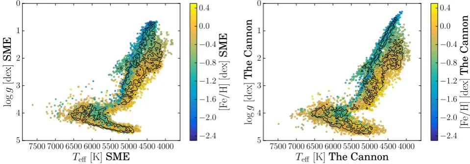
We apply this best-fitting model to the training set spectra as a self-test and subsequently compare the stellar labels from

SME with those estimated by The Cannon in Fig. 8. The

Can-nonreproduces the labels of the training set with negligible

bi-ases and within a scatter ofσ(Teff)= 71 K,σ(logg)=0.25 dex,

σ([Fe/H])=0.1 dex,σ(vmic)=0.06 km s−1,σ(vbroad)=3.1 km s−1,

andσAKS

=0.08 mag. We note that although the Kiel diagrams

of the input and output labels look very similar (see Fig.9), the

scatter values are slightly larger than those of previous analyses

(Martell et al.2017; Sharma et al.2018). While we have not yet

found the reason for this, an explanation could be the expansion of the training set to cover a larger (and hence different) parameter

space, including fast rotators (vbroad>30 km s−1) and metal-poor

stars, which stretches the flexibility of the quadratic model to its

limits. Contrary to the previous models estimated withThe

Can-non for the GALAH survey, we do not fit [α/Fe] as part of the

stellar parameters, as it would interfere with the subsequent

esti-mation of individualα-element abundances, and because it did not

significantly decrease the scatter of the label validation.

3.3.2 The Cannonmodels for element abundances

We reiterate that we use an ensemble of models to infer our elements, based on the six stellar parameters plus one additional element, for all elements. For each training set for each model, we only include those stars in the individual models that have abundance detections

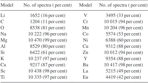
for the respective element. Table2summarizes the relative fractions

of stars in the training set with each element measurement. For each model, we exchange the stellar parameters of SME with those from the self test, before using this model at test time to estimate the individual element abundance. This introduces a minor perturbation to the model (and the stellar labels are slightly different, within the error of the inference). We confirm that the perturbation is minor; the scatter term of the labels from the self test is significantly smaller than before the exchange of stellar parameter labels, see for example

the self-validation for Al in Fig.11.

We emphasize that we have chosen to restrict the abundance de-termination to use only lines of each element being inferred. We

therefore restrictThe Cannon’s model to use only certain

wave-length regions for each element inference (e.g. for [O/Fe] we use

the pixels of the OI7771–5 Å triplet). This masking is achieved

by setting the element-dependent coefficients of the model to zero outside specified regions.

The masks we use for the individual elements are the same as for SME (see Section 3.2.3). This differs from the regularized approach

of Casey et al. (2016), where the model decides which coefficients

of the model to force to 0, but can still identify strongly correlated features. It may be legitimate to learn these correlations and take

advantage of this information (e.g. Ting et al. 2018). Based on

previous analyses, which showed a strong correlation of [α/Fe] and

telluric lines for the GALAH survey, we have chosen to use the most conservative approach for this analysis.

Figure 7. Linear coefficients ofThe Cannonmodel as a function of wavelength across the four HERMES wavelength regions. We show the spectrumf0with labels equivalent to the median of the training set and linear coefficients for five stellar labels. We also include the quadratic coefficient for microturbulence velocity, showing the same pattern as the molecular absorption bands and the scatter of the model. Red dashed lines indicate the Balmer lines.

Figure 8. Comparison of training set labels from SME (input) andThe Cannoninterpolation (output) for the labels of the stellar parameter model, i.e.Teff, logg, [Fe/H],vmic,vbroad, andAKS.

Figure 9. Kiel diagram for the GALAH DR2 training set as determined with SME (left; as input intoThe Cannon) and as reproduced byThe Cannon(right).

3.3.3 The Cannonerrors

The errors reported byThe Cannonare based on the formal

covari-ance errors, which are typically very small. Our total error estimate for each label is based on an additional SNR-dependent

perfor-mance test of the training set for each label. This is estimated by

comparing the difference of the SME input andThe Cannon

out-put as a function of the training set SNR and fitting an exponential function to the mean values within bins of SNR of 25, 50, 75, and

Figur e 10. Spectra o f the giant stars 2 MASS J04262540-7157418 (left-hand panels) and the d w arf star 2MASS J04190076-6040402 (right-hand p anels). Sho w n are th e observ ed spectrum (black) as w ell as the model spectra from The C annon (blue) and the magnified residuals (5 times lar ger in g reen) for dif ferent p arts of the GALAH spectral range. T he top p anels sho w a m agnification o f a part of the b lue arm (CCD 1), while the o ther panels sho w the spectral range of the four bands (CCD 1–4). The C annon is only applied to the second half of the IR-arm. The agreement b etween the n ormalized observ ation and model are o v erall v ery good with mean residuals around 0.005. The lar gest residuals can typically be seen in re gions with imperfect sk yline and telluric line correctio ns in the o bserv ed spectrum.

Table 2. Training set size for individualThe Cannonabundance models, compared to the stellar parameter model with 10 605 spectra.

Model No. of spectra ( per cent) Model No. of spectra ( per cent) Li 1652 (16 per cent) V 3495 (33 per cent) C 1204 (11 per cent) Cr 10 015 (94 per cent) O 8538 (81 per cent) Mn 10 204 (96 per cent) Na 10 222 (96 per cent) Co 5574 (53 per cent) Mg 10 470 (99 per cent) Ni 6388 (60 per cent) Al 8529 (80 per cent) Cu 9312 (88 per cent) Si 6422 (61 per cent) Zn 10 012 (94 per cent) K 10 237 (97 per cent) Y 9354 (88 per cent) Ca 9217 (87 per cent) Ba 10 417 (98 per cent) Sc 10 438 (98 per cent) La 5215 (49 per cent) Ti 10 335 (97 per cent) Eu 4419 (42 per cent)

100. These errors are then summed in quadrature withThe Cannon

covariance errors. We note that this performance test only includes

SNR>25 (as a result of our requirement for the training set spectra

to be of high fidelity). At SNR< 25, the performance test is an

extrapolation and tends to underestimate the errors when compared with the scatter between repeat observations (see Section 4.2).

3.4 Analysis step 3: flagging

To report the quality of both spectra and the spectroscopic analysis,

we are employing several flags, which are summarized in Table5

and explained subsequently.

3.4.1 Flagging of stellar parameter and element abundance estimates

For a given spectrummDR2of the GALAH Data Release 2 with

labelsmDR2, we estimate the label distance to the labelsnTSof the

training set pointsnTSsimilarly to Ho et al. (2017, see their equation

7): D= nTS

mDR2−nTS

2

K2

(11)

For the stellar parameters we use

∈[Teff,logg,[Fe/H], vbroad]

and for the abundance of element X we use

∈[Teff,logg,[Fe/H], vbroad,[X/Fe]].

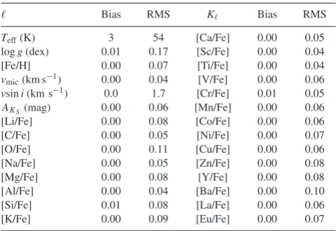
The uncertaintiesKused to estimate the label distances are based

on the RMS of the self-validation as listed in Table3. Subsequently,

we estimate the mean distance of the 10 smallest label distances,

i.e. closest training set points, and raise theflag cannonbitmask

by 1, if this distance is larger than 8 for the stellar parameters (a

mean of 2σfor 4 stellar labels) or 10 for the individual abundances

(a mean of 2σ for 5 stellar labels). We nethertheless also report

the mean label distance to the 10 closest training set points as sp label distanceto allow the exploration of this flag.

Analogous to the analysis with SME (see Section 3.2.3), we estimate if the measured line is a detection or only an upper limit

and raise the bitmask by 2, if the line is<3σ of the flux error, but

at least 5 per cent below the continuum flux.

Additionally, we make use of the χ2_{fit statistic and raise the}

flag cannonbitmask by 4, if the meanχ2_{per pixel (with an}

expectation of 1 for a perfect fit and perfectly known errors) is

either below 0.5 or above 10, both indicating issues with the spectra

or thatThe Cannonmodel cannot describe the given spectrum.

3.4.2 Automated stellar classification with t-SNE

Classification of data is one of the most important steps in any kind of automatic data reduction and analysis. This is especially true in the case where the sheer quantity of collected information prevents us from manually inspecting the data as it comes in, and also when it is not possible to determine all sorts of outliers and unexpected issues a priori. Because the GALAH sample of observed spectra fits this description, it was necessary to develop a semi-automatic classification procedure, which has been presented in Traven et al.

(2017). Here we briefly outline the classification scheme of the

spectra at rest wavelength and its recent improvements.

In order to facilitate the discovery and determination of diverse morphological groups of spectra, we make use of two mathematical techniques, an increasingly more popular dimensionality reduction

method t-SNE (van der Maaten & Hinton 2008), and the

well-established clustering algorithmDBSCAN(Ester et al.1996). These

techniques enable us to condense the information contained in our

entire data set into a two-dimensional map (Fig. 12), where the

spectra are arranged in such a way, that similar ones are grouped to-gether, while there is a clear separation between distinct groups. The strongest features in the data – indicating stellar physical parameters – clearly dictate its global structure, hence the map can be clearly divided between dwarfs and giants or hot and cool stars. Inside these larger groups, there is rich local structure, usually driven by the chemical composition of stars or by any other slowly changing spectral feature. In addition to the influence of stellar parameters, the shape of the projection is also driven by the presence of strong emission lines, or multiple lines from binary and higher order sys-tems.

With the help of the above-described map, we are able to man-ually inspect the structure of our data set and assign classification categories to groups of spectra of interest. To each group in the map, one assigns a category by either looking at the average spectrum of the subset of the group or by the help of previous classification and other existing information/labels. Therefore, with every subsequent classification of the growing data set, it is easier to assign categories; however, new and unexpected features can add to the complexity of the map.

We no longer use the two-step procedure described in Traven et al.

(2017) for producing a t-SNE map of peculiar spectra, since we have

overcome the computational difficulties and can now produce the projection map using all available spectral information of the whole data set in less than a day on a 24-core Xeon node. This became

possible by using the parallel multicore t-SNE code (Ulyanov2016)

and modifying it to remove the limit of overall information that we put into t-SNE. Additionally, we exclude the infrared band as it still suffers from the presence of strong spikes (see Traven et al.

2017), which are now understood and accounted for. The inclusion

of this band would hamper our classification significantly compared to what could be gained from information contained therein.

Fig. 13 presents classification results based on all spectra of

this data release that passed the basic reduction as explained in Section 2.3. We flag all groups of spectra for which a sensible physical category can be determined, however our results are not exhaustive. The population of double-lined spectroscopic binary

stars represents ∼2.2 per cent of the whole data set, down to a

separation of∼10 km s−1_{in the case of most blended double lines.}

Figure 11. Self-validation ofThe Cannonmodel for Al. Table 3. Biases and RMS of the self-validation test.

Bias RMS K Bias RMS

Teff(K) 3 54 [Ca/Fe] 0.00 0.05

logg(dex) 0.01 0.17 [Sc/Fe] 0.00 0.04

[Fe/H] 0.00 0.07 [Ti/Fe] 0.00 0.04

vmic(km s−1) 0.00 0.04 [V/Fe] 0.00 0.06

vsini(km s−1_{) 0.0 1.7 [Cr/Fe] 0.01 0.05}

AKS(mag) 0.00 0.06 [Mn/Fe] 0.00 0.06

[Li/Fe] 0.00 0.08 [Co/Fe] 0.00 0.06

[C/Fe] 0.00 0.05 [Ni/Fe] 0.00 0.07

[O/Fe] 0.00 0.11 [Cu/Fe] 0.00 0.06

[Na/Fe] 0.00 0.05 [Zn/Fe] 0.00 0.08

[Mg/Fe] 0.00 0.08 [Y/Fe] 0.00 0.08

[Al/Fe] 0.00 0.04 [Ba/Fe] 0.00 0.10

[Si/Fe] 0.01 0.08 [La/Fe] 0.00 0.06

[K/Fe] 0.00 0.09 [Eu/Fe] 0.00 0.07

We see a morphological distinction between two larger groups of binaries, which is due to the stronger component being redshifted in one group and blueshifted in the other.

The flagged Hα/Hβ emission stars are very few in our data

set, which is partly because our observations are not focused on young open clusters, but also because a weak emission signature is sometimes not enough for those spectra to stand out in the map. Our observations and data reduction still introduce some issues

that manifest in different features in the spectra and are flagged as problematic, however they are relatively few.

The classification presented in this section serves both as a source of intrinsically interesting objects that can be studied separately (Traven et al., in preparation), and also as a guide to the development and improvement of the reduction and analysis pipeline.

4 VA L I DAT I O N

To validate the results by both SME andThe Cannon, we use a

variety of tests, including the comparisons with fundamental

pa-rameters of theGaiabenchmark stars, repeated observations,

pho-tometric temperatures, asteroseismic surface gravities, open and globular clusters, and other spectroscopic surveys.

4.1 Gaiabenchmark stars

We useGaiabenchmark stars (Jofr´e et al.2014; Heiter et al.2015b)

as one way to validate the accuracy of our stellar parameters. Be-cause of their independently estimated effective temperatures and surface gravities through interferometry and bolometric flux estima-tions, respectively, these parameters are less model-dependent than

our spectroscopically derived ones. In Fig.14, we compare results

with the SME analysis (only based on spectroscopy, as well as with astrometric information) and with the Cannon-based parameters.

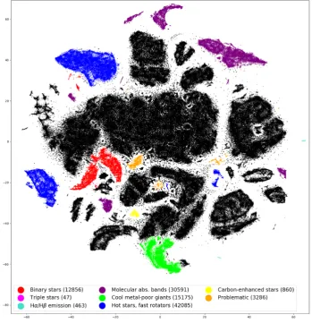
Figure 12. t-SNE projection map of 587 153 spectra. 413 920 of them have reliable stellar parameters derived byThe Cannonpipeline, and others are plotted as black points. The parameters are missing especially not only for hot and cool stars, but also for some binary stars and stars with emission lines, as seen by comparing this figure to Fig.13, where the classification categories are marked. The colour scale is done with 2.5 per cent at both extremes of parameter values truncated for better contrast.

Figure 13. t-SNE projection map, same as Fig.12, except that the points (spectra) are color-coded by classification category. The majority of stars do not show peculiarities and are shown as black dots. The flagged triple stars are few and hardly seen next to the lower left group of binary stars, whereas the Hα/Hβ

emission stars are on the far right and bottom right in the map. The count of spectra for each category is given in the legend.

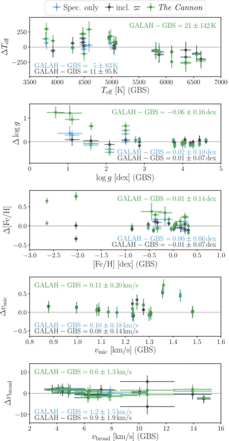
Figure 14. Comparison of GALAH stellar parameters withGaia bench-mark stars (GBS). Shown are differences for the training set (intended as GALAH-Gaia benchmark stars) only based on spectral information (blue), training set including astrometric information (black), andThe Cannon out-put (green).

For the fundamental parameter Teff we find no significant bias

(see offset and dispersion in top panel of Fig.14). For the warmest

Gaiabenchmark stars, we see systematic trends of underestimated

temperatures for both SME analyses, which are propagated byThe

Cannon. For the lumi