1.5 K Using Solar Geoengineering
Anthony C. Jones1 , Matthew K. Hawcroft1, James M. Haywood1,2 , Andy Jones2 , Xiaoran Guo3, and John C. Moore3,4
1College of Engineering, Maths and Physical Sciences (CEMPS), University of Exeter, Exeter, UK,2Earth System and Mitigation Science, Met Office, Exeter, UK,3College of Global Change and Earth System Science, Beijing Normal University, Beijing, China,4Arctic Centre, University of Lapland, Rovaniemi, Finland
Abstract
The 2015 Paris Agreement aims to limit global warming to well below 2 K above preindustrial levels, and to pursue efforts to limit global warming to 1.5 K, in order to avert dangerous climate change. However, current greenhouse gas emissions targets are more compatible with scenarios exhibiting end-of-century global warming of 2.6–3.1 K, in clear contradiction to the 1.5 K target. In this study, we use a global climate model to investigate the climatic impacts of using solar geoengineering by stratospheric aerosol injection to stabilize global-mean temperature at 1.5 K for the duration of the 21st century against three scenarios spanning the range of plausible greenhouse gas mitigation pathways (RCP2.6, RCP4.5, and RCP8.5). In addition to stabilizing global mean temperature and offsetting both Arctic sea-ice loss and thermosteric sea-level rise, we find that solar geoengineering could effectively counteract enhancements to the frequency of extreme storms in the North Atlantic and heatwaves in Europe, but would be less effective at counteracting hydrological changes in the Amazon basin and North Atlantic storm track displacement. In summary, solar geoengineering may reduce global mean impacts but is an imperfect solution at the regional level, where the effects of climate change are experienced. Our results should galvanize research into the regionality of climate responses to solar geoengineering.1. Introduction
In light of the 2015 Paris Agreement that compels participating nations to mitigate greenhouse gas (GHG) emissions at a sufficient rate to avert global warming of 2 K above preindustrial levels (and with the optimal target of avoiding 1.5 K) it has fallen to the climate science community to elucidate plausible mitigation pathways which may limit global warming to 1.5 K (UNFCCC, 2015). Global warming has widely been adopted as a target for GHG mitigation efforts due to its intrinsic relationship with both accumulated car-bon dioxide (CO2) emissions and regional climate changes. The extent to which global-mean temperature targets such as 2 or 1.5 K represent associated climate impacts at a regional level remains uncertain (Knutti et al., 2016).
There remains considerable uncertainty surrounding the feasibility of achieving the 1.5 K target using con-ventional mitigation alone, given historical and present-day GHG emission trends. For example, 56% of coupled global climate models (GCMs) participating in CMIP5 predict that global mean temperature levels will be more than 1.5 K above preindustrial levels by the end of the 21st century under even the most strin-gent RCP2.6 mitigation scenario (e.g., Table 12.3 in Collins et al., 2013). Rogelj et al. (2016) found that current mitigation strategies arising from the Paris agreement (Nationally Determined Contributions [NDCs]) are more consistent with scenarios in which end-of-century global warming reaches 2.6–3.1 K rather than 1.5 K. On the other hand Millar et al. (2017) show that current GCMs overestimate recent historical global temper-ature change and underestimate the cumulative amount of CO2emitted during the industrial period. This latter result suggests that, while stringent cuts in CO2emission will certainly be required, we are not yet at the point where the 1.5 K target is unachievable through conventional mitigation alone. However, the United States—currently the world’s second largest GHG emitter behind China—looks set to withdraw from the Paris agreement (Gies, 2017); an act which signifies the difficulty nations will have in cooperatively adhering to effective mitigation pathways in the long-term future.
10.1002/2017EF000720
Key Points:
• We perform simulations in which solar geoengineering is used to stabilize global warming at 1.5 K above preindustrial levels • Enhanced storm surge activity and
heatwave increases under global warming are effectively counteracted by solar geoengineering
• Solar geoengineering does little to counteract Amazonian hydrological changes and North Atlantic storm track displacement
Supporting Information: • Supporting Information S1.
Correspondence to:
Anthony C. Jones, anthony.jones@ metoffice.gov.uk
Citation:
Jones, A. C., Hawcroft, M. K., Haywood, J. M., Jones, A., Guo, X., & Moore, J. C. (2018). Regional Climate Impacts of Stabilizing Global Warming at 1.5 K Using Solar Geoengineering,Earth’s Future,6, 230–251, https://doi.org/10 .1002/2017EF000720
Received 25 OCT 2017 Accepted 29 JAN 2018
Accepted article online 7 FEB 2018 Published online 19 FEB 2018
© 2018 The Authors.
Various carbon dioxide removal (CDR) methods have been proposed to facilitate conventional mitigation in achieving temperature targets (Shepherd, 2009), and CDR is often implicitly utilized in simulations of ide-alized future scenarios with GCMs (Rogelj et al., 2015). However, it is possible that the potential efficacy of these largely untested CDR approaches has been over-estimated (e.g., Boysen et al., 2017) meaning that cli-mate scenarios dependent on negative CO2emissions (e.g., RCP2.6; van Vuuren et al., 2011) might be overly optimistic and unattainable. This is particularly poignant considering the lack of political traction for CDR investment thus far, for instance, the near ubiquitous omission of CDR in the NDCs (Peters & Geden, 2017). Another important caveat when considering the feasibility of limiting global warming to 1.5 K concerns the fluxes of CO2and methane (CH4) between the atmosphere, the oceans, and the land, with projections largely unconstrained by the CMIP5 GCMs. Therefore, natural GHG fluxes to the atmosphere might aug-ment anthropogenic GHG emissions should the ocean or land become a net carbon source in the future (Friedlingstein et al., 2014). This only adds to the uncertainty of whether effective mitigation and CDR could achieve the Paris temperature targets.
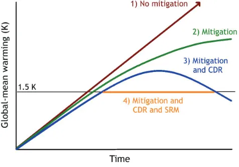
[image:2.594.165.403.304.470.2]In summary, the 1.5 K target appears difficult to achieve by conventional mitigation or using current CDR technology alone without incurring an overshoot, that is, a scenario in which global warming exceeds 1.5 K and is “brought back” to a desired temperature by CDR and mitigation (Scenario 3 in Figure 1). Alterna-tively solar geoengineering, else known as solar radiation management (SRM), has been proposed as a
Figure 1.Schematic of 21st century global warming trends under various scenarios (credit to David MacKay). Note: the similarity between this schematic and Figure 2 of Tilmes et al. (2016).
method for cooling the planet and could be used to stabilize Earth’s tem-perature at 1.5 K instead of incurring a temperature overshoot (Scenario 4 in Figure 1) (Chen & Xin, 2017). SRM refers to a range of climate interventions that aim to increase the reflectivity of the atmosphere or surface to sun-light, hence reducing the absorption of solar energy within the climate sys-tem (Shepherd, 2009). Specific SRM strategies include stratospheric aerosol injection (SAI) which mimics large vol-canic eruptions (Budyko, 1977; Crutzen, 2006), marine cloud brightening which mimics ship tracks and continuously degassing volcanoes (Latham, 1990; Malavelle et al., 2017), and cirrus cloud thinning (CCT) which aims to enhance outgoing terrestrial radiation by reducing high-altitude cirrus coverage (Mitchell & Finnegan, 2009). Note that CCT is technically an example of Longwave Radiation Management rather than SRM as cirrus clouds exert a stronger positive radiative effect from absorbing longwave terrestrial radiation when compared to their negative radiative effect from reflecting shortwave solar radiation. Other SRM strategies such as space mirrors, land albedo modification, and ocean-surface brightening have also been suggested but have received limited attention due to projected costs or projections of large regional climate changes (e.g., Crook et al., 2015; Gabriel et al., 2017; NRC, 2015). A Royal Society report identified SAI as the most promising SRM proposal (Shepherd, 2009); hence we shall solely investigate SAI in this study.
Although the impacts of climate change are felt on the regional scale, certain climate changes such as sea-ice loss, sea-level rise, and changes to the hydrological cycle have global impacts (Collins et al., 2013). Arctic sea ice has retreated over the last four decades due to anthropogenic global warming (Kinnard et al., 2011) and will continue to diminish as the Earth warms, with GCM results suggesting ice-free summers in the Arctic by the end of the century (Mahlstein & Knutti, 2012). The global-mean sea level (GMSL) rose by approximately 1.2 mm/year in the 20th century due to global warming, predominantly via thermosteric effects due to the uptake of heat by the oceans (Hay et al., 2015). A GMSL rise of between 0.26 and 0.55 m for a mitigation-intensive scenario (RCP2.6) and 0.45–0.82 m for a business-as-usual scenario (RCP8.5) is predicted by the end of the 21st century (Church et al., 2013), with additional committed GMSL rise in the longer term due to Antarctic ice loss (Golledge et al., 2015). Sea-level rise will primarily impact coastal populations and small island states, and will increase the risk of flooding and storm surges (Neumann et al., 2015). The hydrological impacts of global warming will vary with region, although precipitation is generally expected to increase which can be explained in part by the Clausius–Clapeyron relationship (i.e., that warmer air holds more water vapor; Collins et al., 2013). For land regions, it is generally predicted that wet regions will get wetter and dry regions will get drier, except for the interesting case of the Amazon basin. Models predict that the Amazonian dry season will be strengthened by global warming, which will concomitantly increase the risk of forest fires and may possibly lead to the degradation or dieback of the tropical rainforest (Boisier et al., 2015; Malhi et al., 2008).
Global warming is also predicted to increase the risk of extreme events such as heatwaves and hurricanes (Emanuel, 2013; Fischer & Knutti, 2015). A heatwave in Europe in the boreal summer of 2003 resulted in 70,000 deaths across 16 countries (Robine et al., 2008), economic losses of $ 10 US billion, extensive forest fires in Greece, Italy, France, Spain, and notably Portugal (covering∼5% of Portuguese territory), and widespread crop and livestock loss (García-Herrera et al., 2010; Schär & Jendritzky, 2004). Contemporaneous forest fires contributed to increased surface ozone emissions resulting in enhanced air pollution across the continent (García-Herrera et al., 2010). Low precipitation rates in spring 2003 resulted in anomalously low soil moisture content across Europe, reducing summertime continental cloud coverage and exerting a positive feedback on the heatwave, concomitantly reducing gross primary productivity (GPP) (Ciais et al., 2005). The 2003 heatwave was not an anomaly—the last decade has seen multiple heatwaves in Europe, including in 2010 and 2015, with the latter leading to the driest and second hottest summer in recent decades (Dong et al., 2016). Heatwaves are subcontinental in extent (a few thousand kilometers), which may limit impacts to certain countries. A heatwave in West Russia in summer 2010 resulted in 55,000 additional deaths, reduced annual crop production by 25% and caused economic losses of $ 15 US billion (Barriopedro et al., 2011). Observations indicate that temperature extremes have increased over land (Brown et al., 2008) and that historical anthropogenic GHG emissions have increased the risk of European heatwaves (Christidis et al., 2011, 2015; Fischer & Knutti, 2015; Stott et al., 2004). GCM simulations indicate that European heatwaves will become longer, more frequent, and more intense in the 21st century under continued global warming (Lau & Nath, 2014; Meehl & Tebaldi, 2004; Russo et al., 2015; Schoetter et al., 2015). Heatwaves are also projected to increase in other regions such as the United States and Australia (Cowan et al., 2014; Lau & Nath, 2012; Meehl & Tebaldi, 2004).
Moving to tropical storms, the 2017 North Atlantic hurricane season has been one of the deadliest and costliest in recent memory with estimated economic damages exceeding $300 US billion, which can be compared to the 2005 season where Hurricane Katrina-related damages exceeded $211 US billion (John-son, 2017). In general, the greatest Hurricane-related risk is from wind-driven storm surges, which primarily threaten low-lying coastal populations including many cities along the south-western coast of the United States (Knutson et al., 2010; Rappaport, 2014). The threat to coastal populations and industry from storm surges is amplified by increases to population density and by sea-level rise. The frequency of intense hur-ricanes in the North Atlantic basin is predicted to increase as a result of global warming, but there is no consensus over the response of overall storm activity to global warming (Emanuel, 2013; Walsh et al., 2016). Coupled with projected sea-level rise and coastal population growth, an increase in the number of intense storms would magnify the impacts of storm-surge events.
the use of GCMs and through validation with postvolcanic eruption observations. These results have shown that a globally uniform SRM deployment would generally be effective at counteracting regional surface temperature and precipitation changes (Jones et al., 2016a; Kravitz et al., 2014), and may enhance net primary productivity by reducing heat stress and enhancing diffuse solar radiation at the surface (Xia et al., 2016). SRM may also be effective at counteracting sea-ice loss and thermosteric sea-level rise (Berdahl et al., 2014; Irvine et al., 2012; Jones et al., 2016a), and offsetting increases to temperature extremes (Curry et al., 2014). However, SRM would also alter stratospheric ozone concentrations by changing stratospheric chemistry and dynamics, which could potentially enhance levels of harmful ultraviolet radiation at the surface (Pitari et al., 2014). Additionally, SRM would not counteract ocean acidification due to elevated CO2 concentrations, and any termination or rapid slowdown of SRM deployment may cause climate change at an unprecedented rate (Jones et al., 2013). Although much research has been devoted to SRM in the last decade, little has been invested in the impacts on specific climate phenomena such as heatwaves or storms (although a few recent studies have begun to explore storm changes [Moore et al., 2015; Jones et al., 2017]). Additionally, no existing modeling study has specifically considered the implications of using SRM to stabilize global-mean temperature at 1.5 K, which is the aim of this study.
We investigate the climatic impacts of SRM in the context of the 1.5 K target by performing simulations with the Hadley Centre Global Environment Model version 2 (HadGEM2-ES). We use three baseline GHG concentrations scenarios from the Representative Concentrations Pathway (RCP) suite: the mitigation and CDR-intensive RCP2.6 (van Vuuren et al., 2011), the middle-of-the-road RCP4.5 (Thomson et al., 2011), and the carbon-intensive RCP8.5 (Riahi et al., 2011). While there are an infinite number of possible future scenar-ios, in essence, these baseline scenarios represent the scenarios “Mitigation and CDR,” “Mitigation,” and “No Mitigation” in Figure 1, respectively. Note, however, that RCP4.5 implicitly assumes a considerable degree of CDR by the end of the century, and is thus not truly representative of standalone mitigation (Thom-son et al., 2011). In our geoengineering scenarios, we assess the repercussions of using SRM to stabilize global warming at 1.5 K while society swiftly transitions onto a mitigation and CDR-intensive pathway (Sce-nario 4 in Figure 1). We also explore sce(Sce-narios in which SRM is used in place of mitigation and/or CDR (i.e., Scenarios 1 and 2 in Figure 1plusSRM, see Section 2). We represent SRM using SAI, that is, by injecting gaseous sulfur dioxide (SO2) into the model stratosphere, following which the SO2oxidizes to form a cloud of light-scattering sulfate (SO4) aerosol (Jones et al., 2010; Kravitz et al., 2011). Our analysis first concentrates on the evolution of globally averaged climate variables such as temperature and precipitation (Section 3.1). We then compare regional climate changes between a recent historical period (1985–2005) and the RCP/SAI simulations evaluated at the end of the 21st century (2070–2099) (Section 3.2). Finally, in Sections 3.3–3.5 we investigate changes to various impactful climate change phenomena—Amazonian drying trends, Euro-pean heatwaves and North Atlantic extreme hurricane frequency—under SAI and global warming. We discuss the implications of our results in Section 4.
2. Model and Methods
The baseline simulations follow CMIP5 protocol (Taylor et al., 2012) and are outlined comprehensively in Jones et al. (2011). Briefly, time-dependent emissions of aerosols (excepting sea-salt and mineral dust), their precursor gases (excepting oceanic DMS), and atmospheric GHG concentrations follow CMIP5 spec-ifications exclusive for each scenario with historical values derived from observations (Meinshausen et al., 2011; Taylor et al., 2012). Tropospheric concentrations of ozone (O3), hydroxyl (OH), hydroperoxyl (HO2), and hydrogen peroxide (H2O2) (which are utilized by CLASSIC as atmospheric oxidants) are directly output from UKCA at each time-step, while stratospheric concentrations of these species are prescribed as monthly mean fields. The suite of simulations comprise a 240-year constant “pre-industrial (1860) conditions” sim-ulation (piControl); a four-member historical (HIST, 1860–2005) ensemble; four-member RCP2.6/ RCP4.5/ RCP8.5 (2005–2099) ensembles following CMIP5 specifications; and four-member RCP2.6/ RCP4.5/ RCP8.5 plus SAI (denoted GEO2.6/ GEO4.5/ GEO8.5) ensembles. We instigate SAI in model year 2020 and inject SO2 at a sufficient rate as to stabilize annual and global-mean warming at 1.5 K above the piControl mean. In the SAI simulations, SO2is injected evenly between 16 and 25 km altitude (six vertical grid cells). As in other SAI studies with HadGEM2-ES (e.g., Haywood et al., 2013; Jones et al., 2010, 2017), we compensate for the lack of an adequately resolved quasi-biennial oscillation (QBO) owing to the limited height of the top of the model by injecting uniformly over the globe rather than injecting at a single point (e.g., Jones et al., 2016b). Our precise method for determining sufficient stratospheric SO2injection rates as to attain 1.5 K is described in Text S1 in the Supporting Information S1.
3. Results
3.1. Annual and Global-Mean Climate Variables
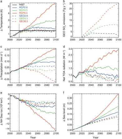
Figure 2 shows various annual and global-mean climate anomalies averaged over each four-member ensemble for each scenario. From Figure 2a, we clearly manage to stabilize global-mean temperature at approximately 1.5 K above piControl levels throughout the 2020–2099 period in the GEO simulations. The GEO2.6, GEO4.5, and GEO8.5 scenarios all succeed in maintaining global-warming since preindustrial times below 1.5 K, while the corresponding RCP2.6, RCP4.5, and RCP8.5 scenarios exceed the 1.5 K target (Table 1). The 2070–2099 RCP anomalies relative to 1986–2005 (Table 1) of 1.46, 2.42, and 4.34 K in RCP2.6, RCP4.5, and RCP8.5, respectively, can be compared to their respective values from the CMIP5 ensemble:+1 [0.3, 1.7] K in RCP2.6,+1.8 [1, 2.5] K in RCP4.5 and 3.4 [2.2, 4.7] K in RCP8.5, where square brackets denote 90% uncertainty ranges. The HadGEM2-ES estimates are therefore at the upper end of the CMIP5 bracket, suggesting a comparatively high transient model sensitivity, as also found by Stott et al. (2013).
In GEO2.6, the SO2injection rate peaks at 3.95 Tg[SO2]/year, then plateaus at 3.5 Tg[SO2]/year. until 2080, then decreases to 1.7 Tg[SO2]/year in 2100 as Earth cools in RCP2.6 due to the implicit upscaling of CDR later in the century (Figure 2b). In GEO4.5, the injection rate increases monotonically to attain a peak value of 10.9 Tg[SO2]/year in 2080 following which it plateaus as global warming in RCP4.5 stabilizes at slightly above 3 K (Figure 2b). In the GEO8.5 scenario, SO2emissions increase quasi-linearly for the duration of the simulations reaching a peak of 29.7 Tg[SO2]/year in 2100. The injection rates given above must be treated with caution due to the simple aerosol microphysics scheme in HadGEM2-ES which does not account for continuous aerosol growth (Text S2 in Supporting Information S1) (Kleinschmitt et al., 2017; Niemeier & Timmreck, 2015). Therefore, the SO2injection rates required to stabilize global warming at 1.5 K may be underestimated in these simulations, as larger-sized aerosol will have a shorter stratospheric lifetime and a greater influence on terrestrial radiation making it less effective at cooling the Earth and hence will require more regular replenishing.
2000 2020 2040 2060 2080 2100 1
2 3 4
5 HISTRCP2.6
RCP4.5
RCP8.5 GEO2.6
GEO4.5
GEO8.5
2000 2020 2040 2060 2080 2100
0 5 10 15 20 25 30
2000 2020 2040 2060 2080 2100
-0.05 0.00 0.05 0.10 0.15 0.20
2000 2020 2040 2060 2080 2100
0.5 1.0 1.5 2.0 2.5 3.0
2000 2020 2040 2060 2080 2100
-14 -12 -10 -8 -6 -4 -2 0
2000 2020 2040 2060 2080 2100
0.00 0.05 0.10 0.15 0.20 0.25 0.30
Δ
Temperature (K)
GEO SO
2
emissions (Tg y
−1
)
Δ
Precipitation (mm d
−1
)
Net TOA radiation (W m
−2
)
Δ
NH Sea ice (10
6 km 2)
Δ
Sea level (m)
Year Year
a b
c d
[image:6.594.169.560.91.535.2]e f
Figure 2.Time series of annual- and global-mean climate variables. (a) near-surface (1.5 m) air temperature anomaly relative to piControl, (b) geoengineering SO2emissions, (c) 5-year smoothed precipitation anomaly relative to HIST (1986–2005), (d) 5-year smoothed net downwelling radiation at the top-of-the-atmosphere (TOA), (e) Northern hemisphere (NH) sea ice anomaly relative to HIST, (f ) thermosteric sea-level anomaly relative to HIST. Vertical dashed lines indicate the initiation of SAI, and the horizontal line in (a) delineates the 1.5 K target.
et al., 2008), and is a robust result of SAI and enhanced stratospheric aerosol burdens following volcanic eruptions (e.g., Tilmes et al., 2013; Trenberth & Dai, 2007). The precipitation trends in GEO2.6 and GEO4.5 are+0.001 and−0.002 mm/day/decade, respectively, which can be compared to−0.016 mm/d/decade in GEO85, suggesting that the nonperfect compensation of global-mean precipitation when temperatures are held fixed by SRM (e.g., Bala et al., 2008) are most evident when the SRM forcing is strong.
3.2. Regional Climate Changes in 2070–2099 Relative to 1986–2005
Table 1.
Global-Mean Temperature Anomalies for: (Column 2) 2020–2099 Relative to the Preindustrial Control Simulation and (Column 3) 2070–2099 Relative to HIST (1986–2005)
Scenario
2020–2099 global warming relative to piControl
2070–2099 global warming relative to 1986–2005
RCP2.6 1.77 [1.74, 1.80] 1.46 [1.40, 1.53]
RCP4.5 2.27 [2.24, 2.29] 2.42 [2.26, 2.56]
RCP8.5 3.29 [3.27, 3.35] 4.34 [4.26, 4.43]
GEO2.6 1.42 [1.37, 1.46] 0.99 [0.87, 1.05]
GEO4.5 1.37 [1.33, 1.40] 1.01 [0.91, 1.10]
GEO8.5 1.49 [1.44, 1.52] 1.08 [0.96, 1.21]
Values in brackets denote the ensemble ranges. The interannual standard deviation of the detrended temperature
time series is approximately±0.1 K in each of the simulations
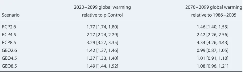
resulting in a more uniform SO4distribution in the NH than the SH (Figure S2 in Supporting Information S1). The greatest SAI-induced cooling is at high latitudes in the NH (Figures 3c,3f,3i), which is influenced not only by the high AODs at these latitudes, but also by the preservation of sea-ice (Figure 2e) and concomitant sup-pression of the sea-ice/snow albedo feedback in the SAI simulations. Nevertheless, SAI does not completely offset the global warming at high NH latitudes relative to HIST (1986–2005) which relates to the reduction in annual-mean sea-ice extent of approximately−4 million km2(Figure 2e). It is also useful to compare the temperature anomalies between the GEO scenarios. The GEO8.5 scenario exhibits slightly greater cooling in the tropics (particularly over the ocean) and greater residual warming at high latitudes relative to GEO4.5 or GEO2.6 (Figures S3 and S4c,d in Supporting Information S1) which reflects the imperfect offset in TOA radiation between SAI and the enhanced greenhouse effect (e.g., Kravitz et al., 2013). Recent studies have shown the strong dependence of the resulting stratospheric AOD on the altitude and latitude of the injec-tion for both volcanos (Jones et al., 2017) and geoengineering (e.g., MacMartin et al., 2017), suggesting that injection strategies could be tailored to optimize the geographic distribution of the cooling (Kravitz et al., 2017). Thus our study represents a single realization of the geographic distribution of AOD and associated cooling; other distributions are certainly possible.
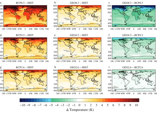
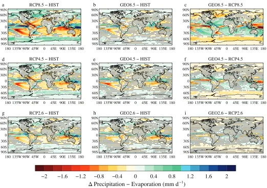
Figure 4 shows the annual-mean precipitation minus evaporation (P-E) changes in the RCP and GEO simu-lations relative to HIST, where the P-E metric is regularly used to measure water availability at the surface, and is more relevant for a climate impacts assessment than standalone precipitation (e.g. Wiltshire et al., 2013). The RCP simulations (Figures 4a,4d,4g) exhibit the archetypal hydrological response to the green-house effect, exemplified by a drying (i.e., a negative P-E anomaly) of the Amazon and tropical oceans, and a moistening (i.e., a positive P-E anomaly) of high-latitudes (e.g., Figure 12.10 in Collins et al., 2013). SAI effec-tively counteracts most of these P-E changes; for instance, the significant high-latitude moistening in RCP8.5 (Figure 4a) is largely offset in GEO8.5 (Figure 4b). In the RCP8.5 scenario, 63% of land regions are affected by significant P-E changes in 2070–2099 relative to HIST, comprising 22% by drying and 42% by wetting (Table S2 in Supporting Information S1). This can be compared to 39% of land regions in the GEO8.5 sce-nario, comprising 14% by drying and 26% by wetting. This indicates that SAI would effectively counteract the annual-mean P-E changes on land under global warming. However, SAI is unable to completely counter-act the P-E reduction in the Amazon basin in GEO8.5 (Figure 4b), and this Amazonian drying is significantly larger in GEO8.5 than GEO2.6 (Figures S5 and S6 in Supporting Information S1). This result compounds the notion that SAI would not be able to completely offset the regional impacts of global warming, in particular impacts to the hydrological cycle (Tilmes et al., 2013). The Amazonian hydrological changes will be explored more in Section 3.3.
180 135W 90W 45W 0 45E 90E 135E 180 90S 60S 30S 0 30N 60N 90N
RCP8.5 − HIST
180 135W 90W 45W 0 45E 90E 135E 180
90S 60S 30S 0 30N 60N 90N
GEO8.5 − HIST
180 135W 90W 45W 0 45E 90E 135E 180
90S 60S 30S 0 30N 60N 90N
GEO8.5 − RCP8.5
180 135W 90W 45W 0 45E 90E 135E 180
90S 60S 30S 0 30N 60N 90N
RCP4.5 − HIST
180 135W 90W 45W 0 45E 90E 135E 180
90S 60S 30S 0 30N 60N 90N
GEO4.5 − HIST
180 135W 90W 45W 0 45E 90E 135E 180
90S 60S 30S 0 30N 60N 90N
GEO4.5 − RCP4.5
180 135W 90W 45W 0 45E 90E 135E 180
90S 60S 30S 0 30N 60N 90N
RCP2.6 − HIST
180 135W 90W 45W 0 45E 90E 135E 180
90S 60S 30S 0 30N 60N 90N
GEO2.6 − HIST
180 135W 90W 45W 0 45E 90E 135E 180
90S 60S 30S 0 30N 60N 90N
GEO2.6 − RCP2.6
a b c
d e f
g h i
−10 −9 −8 −7 −6 −5 −4 −3 −2 −1
0
1
2
3
4
5
6
7
8
9
10
[image:8.594.41.557.87.459.2]Δ
Temperature (K)
Figure 3. Annual-mean near-surface air temperature anomaly evaluated between HIST (1986–2005) and 2070–2099. Hatching indicates regions where differences are insignificant at the 5% level (employing a two-sided Student’st-test).
180 135W 90W 45W 0 45E 90E 135E 180 90S 60S 30S 0 30N 60N 90N
RCP8.5 − HIST
180 135W 90W 45W 0 45E 90E 135E 180
90S 60S 30S 0 30N 60N 90N
GEO8.5 − HIST
180 135W 90W 45W 0 45E 90E 135E 180
90S 60S 30S 0 30N 60N 90N
GEO8.5 − RCP8.5
180 135W 90W 45W 0 45E 90E 135E 180
90S 60S 30S 0 30N 60N 90N
RCP4.5 − HIST
180 135W 90W 45W 0 45E 90E 135E 180
90S 60S 30S 0 30N 60N 90N
GEO4.5 − HIST
180 135W 90W 45W 0 45E 90E 135E 180
90S 60S 30S 0 30N 60N 90N
GEO4.5 − RCP4.5
180 135W 90W 45W 0 45E 90E 135E 180
90S 60S 30S 0 30N 60N 90N
180 135W 90W 45W 0 45E 90E 135E 180
90S 60S 30S 0 30N 60N 90N
180 135W 90W 45W 0 45E 90E 135E 180
90S 60S 30S 0 30N 60N 90N
a
b
c
d
e
f
RCP2.6 − HIST GEO2.6 − HIST GEO2.6 − RCP2.6
g
h
i
2
1.6
1.2
0.8
0.4
0
−0.4
−0.8
−1.2
−1.6
−2
[image:9.594.36.558.86.455.2]Δ
Precipitation − Evaporation (mm d
−1)
Figure 4. Annual-mean precipitation minus evaporation anomaly evaluated between HIST (1986–2005) and 2070–2099. Hatching indicates regions where differences are insignificant at the 5% level (employing a two-sided Student’st-test). (a) RCP8.5-HIST, (d) RCP4.5-HIST, and (g) RCP2.6-HIST; (b), GEO8.5-HIST, (e), GEO4.5-HIST, (h) GEO2.6-HIST; (c), GEO8.5-RCP8.5, (f ), GEO4.5-RCP4.5, (i) GEO2.6-RCP2.6.
assess the daily to seasonal temperature and precipitation responses to SAI, which are outside the scope of this work.
3.3. Hydrology in the Amazon Basin
−0.4 −0.2 0.0 0.2 0.4
0 2 4 6 8
SSA SAU SAF CSA NAU SQF AMZ EQF SEA WAF EAF SAS CAM SAH EAS ENA MED CAS TIB WNA CNA NEU NEE NAS ALA GRL RCP2.6
RCP4.5 RCP8.5
GEO2.6 GEO4.5 GEO8.5
Δ
P−E (mm d
−1
)
Δ
Temperature (K)
Giorgi region
South
North
a
[image:10.594.172.558.97.405.2]b
Figure 5.Annual land-mean (a) precipitation minus evaporation (P-E) and (b) temperature anomalies for 26 Giorgi regions (Table S1 in Supporting Information S1), evaluated between HIST (1986–2005) and 2070–2099. Horizontal black lines denote±1 standard deviation of the interannual precipitation/temperature in HIST. The regions comprise: Southern South America (SSA), Southern Australia (SAU), Southern Africa (SAF), Central South America (CSA), Northern Australia (NAU), Southern Equatorial Africa (SQF), Amazon Basin (AMZ), Equatorial Africa (EQF), South Eastern Asia (SEA), Western Africa (WAF), Eastern Africa (EAF), Southern Asia (SAS), Central America (CAM), Sahara (SAH), Eastern Asia (EAS), Eastern North America (ENA), Mediterranean Basin (MED), Central Asia (CAS), Tibet (TIB), Western North America (WNA), Central North America (CNA), Northern Europe (NEU), North Eastern Europe (NEE), Northern Asia (NAS), Alaska (ALA), and Greenland (GRL).
Halladay and Good (2017) investigated the Amazonian hydrological response to global warming using HadGEM2-ES and found that evapotranspiration changes were primarily attributable to plant physiological changes and reduced canopy water content. It is instructive to perform a similar investigation using the RCP and SAI simulations. Figure 6 shows the annual-mean precipitation, evaporation, and P-E anomalies in the RCP and SAI simulations in 2070–2099 relative to HIST. It is clear that most of the hydrological changes in the RCP simulations (Figures 6a-6i) exhibit an east–west gradient, with greater perturbations in East Amazonia (60∘–48∘W, 12∘S–3∘N), despite the baseline precipitation being greater in the west (Figure S10 in Support-ing Information S1). Precipitation reductions over East Amazonia in the RCP scenarios are partially offset by reduced evaporation, which limits changes to surface water availability. Of the RCP scenarios, RCP8.5 exhibits the largest reductions in precipitation, evaporation, and P-E (Figures 6a-6c). SAI appears to partially counteract the precipitation, evaporation, and P-E changes over East Amazonia relative to the correspond-ing RCP scenario, but also reduces precipitation, evaporation, and P-E over West Amazonia (72∘–60∘W, 12∘S–3∘N), which is less apparent in the RCP scenarios. Of the SAI scenarios, GEO8.5 exhibits the largest precipitation and evaporation changes relative to HIST (Figures 6j and 6k).
2 1.6 1.2 0.8 0.4 0 −0.4 −0.8 −1.2 −1.6 −2
mm d−1
Δ Precipitation Δ Evaporation Δ Precip−Evap
RCP8.5
RCP4.5
RCP2.6
GEO8.5
GEO4.5
GEO2.6
a b c
d e f
g h i
)
j k l
m n o
[image:11.594.167.559.105.676.2]p q r
Figure 6. Annual-mean precipitation (P), evaporation (E), and P-E differences in the Amazon between 2070–2090 and HIST
simulations (Figures S11 and S12 in Supporting Information S1), which is consistent with a reduction in P-E. SAI is generally ineffective at counteracting changes to GPP, stomatal conductance, and surface runoff in these simulations, except in the case of GEO8.5 where the surface cooling stops a temperature threshold from being reached which ultimately reduces GPP in RCP8.5 (Figure S12 in Supporting Information S1; Hal-laday & Good, 2017). The sensitivity of Amazonian hydrology to atmospheric CO2concentrations appears to at least partially explain why the precipitation and evaporation reductions are greater in GEO8.5 than those in GEO4.5 or GEO2.6, and why SAI is ineffective at counteracting changes to Amazonian hydrology. It is also important to investigate whether the Amazon hydrological changes may relate to atmospheric dynamical changes. In the annual mean, the ITCZ is enhanced over the ocean, but not the land, in the RCP simulations (Figures S6a and S6b in Supporting Information S1). The relationship between cross-equatorial energy transport and zonal mean tropical precipitation is well established (e.g., Hawcroft et al., 2017; Haywood et al., 2013, 2016; Schneider et al., 2014), with the ITCZ moving toward the warmer hemisphere, though this does not appear to be the mechanism operating in this case, since cross-equatorial atmo-spheric energy transport changes very little in either the RCP or GEO simulations (Figure S13 in Supporting Information S1). Instead, a reorganization of tropical atmospheric circulation based on changes in SST patterns is one possible driver of reduced precipitation in the Amazon, alongside the aforementioned plant physiological effect.
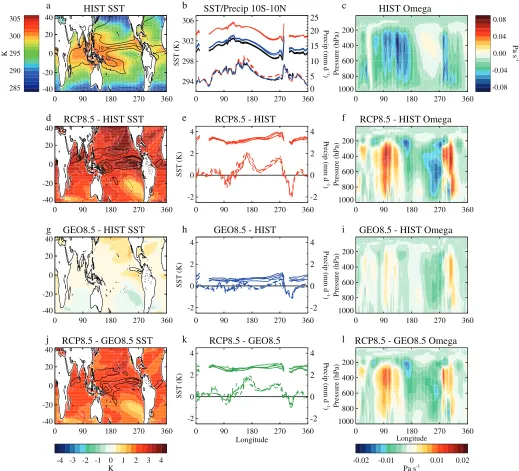
The spatial patterns of RCP8.5 precipitation anomalies in South America are remarkably similar to recent EN events (Jiménez-Muñoz et al., 2016) and in Figure 7d, an EN-like reduction in the cold tongue and reorganization of tropical Pacific precipitation is observed. Meridional mean near-equatorial (10∘S–10∘N) SST changes (Figure 7b and 7e) have limited zonal variability; with relatively uniform SST meridional mean increases across the tropics. Enhancement of precipitation in the east Pacific is clear (Figure 7e) and is associated with enhanced convergence and convection in the cold tongue region. The reorga-nization of the Walker circulation associated with these shifts leads to forced descent over the Amazon (Figure 7f, where positive values of omega indicate descent), which is only partly compensated in the GEO8.5 scenario. Changes in the annual cycle of precipitation in the east Pacific and Amazon (Figure S14 in Supporting Information S1) further support this analysis, with precipitation reductions in the Amazon most pronounced in the boreal summer, when east Pacific precipitation exhibits the largest changes. The reduction in Amazonian precipitation in Figure 6 therefore appears to be driven by plant physiological changes and by circulation anomalies associated with relatively subtle changes to regional SST patterns, rather than a wholesale northward shift in zonal mean precipitation associated with changes in the global energy budget and meridional energy transport.
3.4. European Heatwaves
Heatwaves are defined as extended periods of above-average temperatures and are often accompanied by drought-like conditions. It has been established that European heatwave incidence is related to synop-tic climate phenomena such as extratropical cyclone tracks, the NH mid-latitude jet stream (Kysel´y, 2008; Stefanon et al., 2012) and atmospheric blocking events which may also induce cold spells (Brunner et al., 2017). Additionally, a prerequisite for heatwave formation may be drought-like conditions (Stefanon et al., 2012), and a positive feedback on the heatwave may be induced by simultaneous precipitation reductions such as observed during the 2015 European heatwave (Dong et al., 2016). As European heatwaves are high-impact events with significant societal and agricultural consequences, it is instructive to investigate heatwave changes in the RCP and GEO simulations.
0 90 180 270 360 -40 -20 0 20 40 HIST SST 10 10 285 290 295 300 305
0 90 180 270 360
-40 -20 0 20 40
RCP8.5 - HIST SST
0 90 180 270 360
-40 -20 0 20 40
GEO8.5 - HIST SST
0 90 180 270 360
-40 -20 0 20 40
RCP8.5 - GEO8.5 SST
-4 -3 -2 -1 0 1 2 3 4
SST/Precip 10S-10N
0 90 180 270 360
294 298 302 306 0 5 10 15 20 25
RCP8.5 - HIST
0 90 180 270 360
-2 0 2 4 -2 0 2 4
GEO8.5 - HIST
0 90 180 270 360
-2 0 2 4 -2 0 2 4
RCP8.5 - GEO8.5
0 90 180 270 360
Longitude -2 0 2 4 -2 0 2 4
0 90 180 270 360
1000 800 600 400 200 HIST Omega -0.08 -0.04 0.00 0.04 0.08
0 90 180 270 360
1000 800 600 400 200
RCP8.5 - HIST Omega
0 90 180 270 360
1000 800 600 400 200
GEO8.5 - HIST Omega
0 90 180 270 360
1000 800 600 400 200
RCP8.5 - GEO8.5 Omega
-0.02 -0.01 0 0.01 0.02
SST (K)
SST (K)
SST (K)
SST (K)
Precip (mm d
-1
)P
recip (mm d
-1
)P
recip (mm d
-1
)P
recip (mm d
-1 ) Pressure (hPa) Pressure (hPa) Pressure (hPa) Pressure (hPa) K Pa s -1 Longitude
K Pa s-1
a b c
d e f
g h i
[image:13.594.36.555.90.561.2]j k l
Figure 7. Annual-mean (a) sea-surface temperatures (SSTs) (colored contours, K) and precipitation (black lines, interval 5 mm/day) in the HIST simulation with differences to (d) RCP8.5, (g) GEO8.5, and (j) the difference between RCP8.5 and GEO8.5 (precipitation contours at−3,−2,−1, 1, 2, 3 mm/day with negative values dashed). (b) Mean near-equatorial (10∘S–10∘N) SSTs (ocean only, solid lines) and precipitation (land and ocean, dashed lines) for HIST (black), RCP8.5 (red), and GEO8.5 (blue), with differences from HIST to (e) RCP8.5, (h) GEO8.5, and (k) the difference between RCP8.5 and GEO8.5. (c) Mean near-equatorial (10∘S–10∘N) vertical descent rate (omega) (land and ocean, Pa/s) for HIST, with differences from HIST to (f ) RCP8.5, (i) GEO8.5, and (l) the difference between RCP8.5 and GEO8.5.
RCP8.5
Mean = 62.68
RCP4.5
Mean = 31.72
RCP2.6
Mean = 17.04
GEO8.5
Mean = 14.76
GEO4.5
Mean = 14.42
GEO2.6
Mean = 11.59
5 10 15 20 25 30 35 40 45 50 55 60 65 70 75 80 85 90
Δ Hot days (> Tx95) per year
a d
b e
[image:14.594.165.561.85.548.2]c f
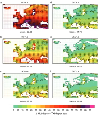
Figure 8.Differences in annual frequency of hot days (i.e., days in May–September (MJJAS) in which the daily maximum temperature exceeds the 95% quantile of the HIST (1986–2005) MJJAS daily maximum temperature distribution (Tx95)) between 2070–2099 and HIST for (a) RCP8.5, (b) RCP4.5, (c) RCP2.6, (d) GEO8.5, (e) GEO4.5, and (f ) GEO2.6. Black dots indicate where differences are significant at the 5% level (employing a two-sided Student’st-test).
RCP8.5
Mean = -0.12
RCP4.5
Mean = -0.04
RCP2.6
Mean = 0.01
GEO8.5
Mean = -0.07
GEO4.5
Mean = -0.04
GEO2.6
Mean = 0.02
1.0 0.8 0.6 0.4 0.2 0.0 -0.2 -0.4 -0.6 -0.8 -1.0
Δ
May−Sep Precip. (mm d
−1)
(a)
(b)
(c)
(d)
(e)
[image:15.594.167.560.86.504.2](f)
Figure 9. May–September mean precipitation anomaly (mm/day) between 2070–2099 and HIST (1986–2005) for (a) RCP8.5, (b) RCP4.5, (c) RCP2.6, (d) GEO8.5, (e) GEO4.5, and (f ) GEO2.6. Hatching indicates regions where differences are insignificant at the 5% level (employing a two-sided Student’st-test).
(Figure S19 in Supporting Information S1), which suggests that changes to summertime surface water content in Europe would be effectively counteracted by SAI. Although the 2003 European heatwave was preceded by low precipitation in spring, which intensified that particular heatwave (García-Herrera et al., 2010), we do not see the same robust precipitation response in the RCP or GEO simulations (Figure S20 in Supporting Information S1). Instead, the mean precipitation-cloud-radiative feedback appears to occur simultaneously to the peak heatwave season (MJJAS) (Figure 9), such as observed during the summer 2015 European heatwave (Dong et al., 2016). However, the use of seasonal-mean precipitation and P-E metrics as used here may be less informative than investigating hydrology coincident with each heatwave.
3.5. Extreme Hurricane Frequency in the North Atlantic
In the North Atlantic, historical trends in meteorological variables such as global-mean surface tempera-ture and temperatempera-ture in the hurricane main development region (MDR, [85∘W–20∘W and 10∘N–20∘N]) are well correlated with tropical storm surges (Grinsted et al., 2013). This is because a warm ocean sur-face provides a burgeoning vortex with energy, increasing the potential intensity and lifetime of the storm. Therefore, it is instructive to utilize established statistical relationships between meteorological conditions and storm surges to assess how the frequency of the most intense storms may change in the RCP and GEO scenarios.
Two recent studies have also investigated North Atlantic storm changes under SAI. Moore et al. (2015) used the same statistical model as used here, applied to multimodel GeoMIP (Kravitz et al., 2011) output, to show that SAI could counteract increases in Katrina-sized storm surges resulting from global warming. Jones et al. (2017) investigated North Atlantic storm changes in simulations conducted with HadGEM2-ES (also used here) by employing a variety of different storm-identification methods. A clear disparity was identified between the results of explicit storm tracking and statistical-dynamical downscaling, notably that under global warming storm activity is predicted to decrease using the former method and increase using the latter method (Jones et al., 2017). We utilize an alternative statistical algorithm to Jones et al. (2017) which relates storm-surge activity to MDR-mean SSTs from observations. Historical storm-surge activity is inferred from a homogeneous storm surge time series, developed using daily tidal gauge data from six stations along the south western coast of the United States (Grinsted et al., 2012). This homogeneous surge index has been found to be well correlated with historical U.S. storm landfalls and associated economic damages (Grinsted et al., 2012). A nonstationary generalized extreme value (GEV) model with shape, scale, and loca-tion parameters dependent on observed MDR temperatures is fit to the surge index using a Monte Carlo Markov Chain approach (see Grinsted et al., 2013; Moore et al., 2015). Specifically, we use three different covariates to explore storm changes: average surface temperature in the MDR, globally averaged surface temperature, and global spatial-grids of surface temperature (where the weighting for each grid-cell relates to its area and relative predictive skill) (see Grinsted et al., 2013). Finally, the GEV models are applied to the HadGEM2-ES simulated meteorology and storm surges that exceed the maximum observed storm surge following Hurricane Katrina are counted (Moore et al., 2015).
RCP8.5
1850 1900 1950 2000 2050 2100 Year
0.1 1.0 10.0 100.0
Katrinas dec
-1
Katrinas dec
-1
Gridded
Global
MDR
RCP4.5
1850 1900 1950 2000 2050 2100 Year
0.1 1.0 10.0 100.0
Katrinas dec
-1
RCP2.6
1850 1900 1950 2000 2050 2100 Year
0.1 1.0 10.0 100.0
Katrinas dec
-1
GEO8.5
1850 1900 1950 2000 2050 2100 Year
0.1 1.0 10.0 100.0
GEO4.5
1850 1900 1950 2000 2050 2100 Year
0.1 1.0 10.0 100.0
Katrinas dec
-1
GEO2.6
1850 1900 1950 2000 2050 2100 Year
0.1 1.0 10.0 100.0
Katrinas dec
-1
a
d
b
e
[image:17.594.170.558.89.531.2]c
f
Figure 10.Number of Katrina-sized surge events per decade under the projected changes in MDR-mean (red lines), global-mean (black lines) and global gridded temperature (dark blue lines) using the ensemble average of the RCP and GEO simulations. The vertical dashed line indicates the initiation of SAI. Blue shaded areas are confidence intervals (5–16–84–95%) for the global gridded temperature model. Lines are smoothed by 10-year centered moving averages.
reduced in the GEO simulations relative to the RCP simulations (Figure 2e and 2f ), which would concomi-tantly reduce the risk of flooding from storm surges in the GEO simulations (Woodruff et al., 2013). Further simulations with high-resolution climate models and explicit storm-tracking algorithms would provide an interesting counterpart to this preliminary study and would confirm the suitability of using temperature indices as predictors of hurricane frequency.
4. Conclusions
−1.0 −0.5 0.0 0.5 1.0
−1.0 −0.5 0.0 0.5 1.0
Normalized climate changes
Δ
T
Δ
P−E (Land)
Δ
NH sea ice
Δ
GMSL
Δ
P−E (WAMZ)
Δ
P−E (EAMZ)
Δ
EUR hot days
Δ
NATL storms
2.
6
4.5
8.5
2.6
4.5
8.5
2.6
4.5
8.5
2.6
4.
5
8.5
1
σ
a
b
c
d
[image:18.594.173.560.89.345.2]e
f
g
h
Figure 11.Normalized climate changes (divided by maximum absolute anomaly) between 2070–2099 and 1986–2005: (a) global-mean temperature (max= +4.3 K), (b) land-mean precipitation minus evaporation (P-E) (max= +0.034 mm/day), (c) NH sea-ice extent (max= −12×106km2), (d) global-mean sea level (max= +0.265 m), (e) West Amazonian P-E (max= −0.38 mm/day), (f ) East Amazonian P-E (max= −0.72 mm/day), (g) European hot days (max= +62.7 days), (g) Extreme storm surges in the North Atlantic (max= +16.4 Katrinas/decade). Arrows point from the RCP to the GEO scenario. Dotted lines indicate±1 interannual standard deviation in the HIST period.
changes over the Amazon (Figures 11b,11e, and 11f ), which we attribute to the plant physiological response to CO2and to a regional dynamical response related to subtle SST changes in the Pacific (Figure 7). We also find that European heatwave enhancements are suppressed more effectively when SAI is applied to a mitigation-intensive scenario (GEO2.6) than a carbon-intensive scenario (GEO8.5), which we attribute to the greater residual warming at high latitudes in GEO8.5 and a resultant poleward migration of the extra-tropical storm tracks. However, the heatwave differences between the SAI scenarios are negligible when compared to the heatwave changes in the RCP8.5 and RCP4.5 scenarios (Figure 11g), and SAI is generally effective at offsetting increases to European heatwaves. Generally, our work exposes the naivety of a single global mean temperature metric as a threshold for “dangerous global warming” as this does not account for deleterious impacts on other aspects of regional climate and other risks (e.g. Robock et al., 2008). Even without the Amazonian drying trends and heatwave disparities, the GEO8.5 scenario is inherently riskier than GEO4.5 or GEO2.6 due to the “termination effect”, that is, that should SAI be rapidly terminated, the climate would swiftly rebound to its base state (Jones et al., 2013). As GEO8.5 is consistently further away from its base state climate than GEO4.5 or GEO2.6, the termination effect would be much greater in GEO8.5 and such rates of climate change may be beyond the adaptive capacity of certain ecosystems (Jones et al., 2013). Hence, despite GEO8.5 exhibiting a similar global and annual mean climate to GEO4.5 and GEO2.6 at the end of the century; the unprecedented risk attached to such a scenario should prove an effective deterrent for over-reliance on solar geoengineering at the expense of mitigation and CDR. Nevertheless, the effectiveness of SAI at counteracting deleterious climate impacts such as sea-level rise, enhanced hurricane frequency, and European heatwave frequency should galvanize further research into SAI, which may prove a useful tool for offsetting certain severe climate changes in a temperature overshoot scenario.
aerosol’s light-scattering efficiency and stratospheric residence times (Kleinschmitt et al., 2017; Niemeier & Timmreck, 2015); effects which are not accounted for by HadGEM2-ES. However, a set of recent simula-tions with the WACCM climate model were able to stabilize the global-mean temperature at 2020 levels against RCP8.5 using SAI (Kravitz et al., 2017; MacMartin et al., 2017). It is therefore important that the geoengineering research community repeats these simulations using other GCMs to test the robustness of our results—preferably within the GeoMIP framework (Kravitz et al., 2011). Nevertheless, many of our inferences concerning climate impacts (e.g., to the hydrological cycle) are backed up by a large amount of scientific literature on solar geoengineering that has developed in the last 15 years, enhancing confidence in the results.
Our decision to investigate European heatwaves and North Atlantic hurricane frequency relates primarily to the authors’ previous work (Jones et al., 2017; Moore et al., 2015). In considering three regional climate impact case studies in this paper, we accept that these results are preliminary and are based on a single set of experiments with one climate model. The critical point that is made in this work, with respect to regional impacts, is that even if global indices can be stabilized by SAI interventions, this is not a complete solution. Previous studies have suggested that SAI deployment may benefit some regions more than others (Kravitz et al., 2014; Ricke et al., 2010), which is likely to make any interventions politically charged. However, with the exception of P-E for western Amazonia (Figure 11e), our simulations indicate a universal reduction in detri-mental impacts when compared to RCP scenarios. The preliminary climate impacts assessment undertaken in this study should be extended by future studies to assess potentially deleterious climatic phenomena in other regions; for instance the intensity of the Asian monsoon may weaken under SAI (Robock et al., 2008), although our simulations show little deleterious impact (SAS, SEA, Figure 5a). Additionally, some of the climate impacts metrics that we have utilized are empirical, for instance using temperature as the sole predictor variable for the heatwave and storm analyses in Sections 3.4 and 3.5. Therefore, future impacts assessments may wish to develop our work by employing, for example, heat stress or drought indices to measure heatwave frequency, and by explicitly tracking storms in GCM output to measure storm activity (e.g., Jones et al., 2017). Critically, the regional climate impacts of solar geoengineering, including impacts on specific phenomena such as heatwaves, must be explored in greater detail in future studies.
References
Bala, G., Duffy, P. B., & Taylor, K. E. (2008). Impact of geoengineering schemes on the global hydrological cycle.Proceedings of the National Academy of Sciences of the United States of America,105, 7664–7669. https://doi.org/10.1073/pnas.0711648105
Barriopedro, D., Fischer, E. M., Luterbacher, J., Trigo, R. M., & García-Herrera, R. (2011). The hot summer of 2010: Redrawing the temperature record map of Europe.Science,332, 220–224. https://doi.org/10.1126/science.1201224
Becker, A., Finger, P., Meyer-Christoffer, A., Rudolf, B., Schamm, K., Schneider, U., & Ziese, M. (2013). A description of the global land-surface precipitation data products of the global precipitation climatology Centre with sample applications including centennial (trend) analysis from 1901–present.Earth System Science Data,5, 71–99. https://doi.org/10.5194/essd-5-71-2013
Bellouin, N., Boucher, O., Haywood, J., Johnson, C., Jones, A., Rae, J., et al. (2007).Improved representation of aerosols for HadGEM2(Hadley Centre Technical Note No. 73).
Bellouin, N., Rae, J., Jones, A., Johnson, C., Haywood, J., & Boucher, O. (2011). Aerosol forcing in the climate model Intercomparison project (CMIP5) simulations by HadGEM2-ES and the role of ammonium nitrate.Journal of Geophysical Research,116, D20206. https:// doi.org/10.1029/2011JD016074
Berdahl, M., Robock, A., Ji, D., Moore, J. C., Jones, A., Kravitz, B., & Watanabe, S. (2014). Arctic cryosphere response in the geoengineering model intercomparison project G3 and G4 scenarios.Journal of Geophysical Research – Atmospheres,119, 1308–1321. https://doi.org/ 10.1002/2013JD020627
Boisier, J. P., Ciais, P., Ducharne, A., & Guimberteau, M. (2015). Projected strengthening of Amazonian dry season by constrained climate model simulations.Nature Climate Change,5, 656–660. https://doi.org/10.1038/nclimate2658
Boysen, L. R., Lucht, W., Gerten, D., Heck, V., Lenton, T. M., & Schellnhuber, H. J. (2017). The limits to global-warming mitigation by terrestrial carbon removal.Earth’s Future,5, 463–474. https://doi.org/10.1002/2016EF000469
Brown, S. J., Caesar, J., & Ferro, C. A. T. (2008). Global changes in extreme daily temperature since 1950.Journal of Geophysical Research,
113, D05115. https://doi.org/10.1029/2006JD008091
Brunner, L., Hegerl, G. C., & Steiner, A. K. (2017). Connecting atmospheric blocking to European temperature extremes in Spring.Journal of Climate,30, 585–594. https://doi.org/10.1175/JCLI-D-16-0518.1
Budyko, M. I. (1977).Climatic changes. Washington, DC, 244 pp.: American Geophysical Union. https://doi.org/10.1029/SP010 Chadwick, R., Douville, H., & Skinner, C. B. (2017). Timeslice experiments for understanding regional climate projections: Applications to
the tropical hydrological cycle and European winter circulation.Climate Dynamics,49, 3011–3029. https://doi.org/10.1007/s00382-016-3488-6
Chen, Y., & Xin, Y. (2017). Implications of geoengineering under the 1.5∘C target: Analysis and policy suggestions.Advances in Climate Change Research,8(2017), 123–129. https://doi.org/10.1016/j.accre.2017.05.003
Christidis, N., Jones, G. S., & Stott, P. A. (2015). Dramatically increasing chance of extremely hot summers since the 2003 European heatwave.Nature Climate Change,5, 46–50. https://doi.org/10.1038/nclimate2468
Christidis, N., Stott, P., & Brown, S. (2011). The role of human activity in the recent warming of extremely warm daytime temperatures.
Journal of Climate,24(7), 1922–1930. https://doi.org/10.1175/2011JCLI4150.1 Acknowledgments
Church, J. A., Clark, P. U., Cazenave, A., Gregory, J. M., Jevrejeva, S., Levermann, A., et al. (2013). Sea level change. In T. F. Stocker, D. Qin, G.-K. Plattner, M. Tignor, S. K. Allen, J. Boschung, et al. (Eds.),Climate Change 2013: The Physical Science Basis. Contribution of Working Group I to the Fifth Assessment Report of the Intergovernmental Panel on Climate Change. Cambridge, England: Cambridge University Press. Ciais, P., Reichstein, M., Viovy, N., Granier, A., Ogee, J., Allard, V., et al. (2005). Europe-wide reduction in primary productivity caused by the
heat and drought in 2003.Nature,437, 529–533. https://doi.org/10.1038/nature03972
Collins, M., Knutti, R., Arblaster, J., Dufresne, J.-L., Fichefet, T., Friedlingstein, P., et al. (2013). Long-term climate change: Projections, commitments and irreversibility. In T. F. Stocker, D. Qin, G.-K. Plattner, M. Tignor, S. K. Allen, J. Boschung, et al. (Eds.),Climate Change 2013: The Physical Science Basis. Contribution of Working Group I to the Fifth Assessment Report of the Intergovernmental Panel on Climate Change. Cambridge, England: Cambridge University Press.
Collins, W. J., Bellouin, N., Doutriaux-Boucher, M., Gedney, N., Halloran, P., Hinton, T., et al. (2011). Development and evaluation of an earth-system model – HadGEM2.Geoscientific Model Development,4, 1051–1075. https://doi.org/10.5194/gmd-4-1051-2011 Cowan, T., Purich, A., Perkins, S., Pezza, A., Boschat, G., & Sadler, K. (2014). More frequent, longer and hotter heat waves for Australia in the
21st century.Journal of Climate,27, 5851–5871. https://doi.org/10.1175/JCLI-D-14-00092.1
Crook, J. A., Jackson, L. S., Osprey, S. M., & Forster, P. M. (2015). A comparison of temperature and precipitation responses to different earth radiation management geoengineering schemes.Journal of Geophysical Research – Atmospheres,120, 9352–9373. https://doi.org/10 .1002/2015JD023269
Crutzen, P. (2006). Albedo enhancement by stratospheric sulfur injections: A contribution to resolve a policy dilemma?Climatic Change,
77(3), 211–220. https://doi.org/10.1007/s10584-006-9101-y
Curry, C. L., Sillmann, J., Bronaugh, D., Alterskjaer, K., Cole, J. N. S., Ji, D., et al. (2014). A multimodel examination of climate extremes in an idealized geoengineering experiment.Journal of Geophysical Research – Atmospheres,119, 3900–3923. https://doi.org/10.1002/ 2013JD020648
Dee, D. P., Uppala, S. M., Simmons, A. J., Berrisford, P., Poli, P., Kobayashi, S., et al. (2011). The ERA-interim reanalysis: Configuration and performance of the data assimilation system.Quarterly Journal of the Royal Meteorological Society,137, 553–597. https://doi.org/10 .1002/qj.828
Dong, B., Sutton, R., Shaffrey, L., & Wilcox, L. (2016). The 2015 European heat wave, [in “explaining extremes of 2015 from a climate perspective”].Bulletin of the American Meteorological Society,97(12), S14–S18. https://doi.org/10.1175/BAMS-D-16-0140.1 Emanuel, K. A. (2013). Downscaling CMIP5 climate models shows increased tropical cyclone activity over the 21st century.Proceedings of
the National Academy of Sciences,110(30), 12,219–12,224. https://doi.org/10.1073/pnas.1301293110
Fischer, E. M., & Knutti, R. (2015). Anthropogenic contribution to global occurrence of heavy-precipitation and high-temperature extremes.Nature Climate Change,5, 560–564. https://doi.org/10.1038/nclimate2617
Friedlingstein, P., Meinshausen, M., Arora, V. K., Jones, C. D., Anav, A., Liddicoat, S. K., & Knutti, R. (2014). Uncertainties in CMIP5 climate projections due to carbon cycle feedbacks.Journal of Climate,27, 511–526. https://doi.org/10.1175/JCLI-D-12-00579.1
Gabriel, C. J., Robock, A., Xia, L., Zambri, B., & Kravitz, B. (2017). The G4Foam experiment: Global climate impacts of regional ocean albedo modification.Atmospheric Chemistry and Physics,17, 595–613. https://doi.org/10.5194/acp-17-595-2017
García-Herrera, R., Díaz, J., Trigo, R. M., Luterbacher, J., & Fischer, E. M. (2010). A review of the European summer heat wave of 2003.Critical Reviews in Environmental Science and Technology,40(4), 267–306. https://doi.org/10.1080/10643380802238137
Gies, E. (2017). Businesses lead where US falters.Nature Climate Change,7, 543–546. https://doi.org/10.1038/nclimate3360 Giorgi, F. (2006). Climate change hot-spots.Geophysical Research Letters,33, L08707. https://doi.org/10.1029/2006GL025734 Golledge, N. R., Kowalewski, D. E., Naish, T. R., Levy, R. H., Fogwill, C. J., & Gasson, E. G. W. (2015). The multi-millennial Antarctic
commitment to future sea-level rise.Nature,526, 421–425. https://doi.org/10.1038/nature15706
Grinsted, A., Moore, J. C., & Jevrejeva, S. (2012). Homogeneous record of Atlantic hurricane surge.Proceedings of the National Academy of Sciences,109(48), 19,513–19,514. https://doi.org/10.1073/pnas.1216735109
Grinsted, A., Moore, J. C., & Jevrejeva, S. (2013). Projected Atlantic hurricane surge threat from rising temperatures.Proceedings of the National Academy of Sciences of the United States of America,110(14), 5369–5373. https://doi.org/10.1073/pnas.1209980110 Halladay, K., & Good, P. (2017). Non-linear interactions between CO2radiative and physiological effects on Amazonian evapotranspiration
in an earth system model.Climate Dynamics,49, 2471–2490. https://doi.org/10.1007/s00382-016-3449-0
Harris, P. P., Huntingford, C., & Cox, P. M. (2008). Amazon Basin climate under global warming: The role of the sea surface temperature.
Philosophical Transactions of the Royal Society B,363, 1753–1759. https://doi.org/10.1098/rstb.2007.0037
Hawcroft, M., Haywood, J. M., Collins, M., Jones, A., Jones, A. C., & Stephens, G. (2017). Southern Ocean albedo, inter-hemispheric energy transports and the double ITCZ: Global impacts of biases in a coupled model.Climate Dynamics,48(7–8), 2279–2295. https://doi.org/ 10.1007/s00382-016-3205-5
Hay, C. C., Morrow, E., Kopp, R. E., & Mitrovica, J. X. (2015). Probabilistic reanalysis of twentieth-century sea-level rise.Nature,517, 481–484. https://doi.org/10.1038/nature14093
Haylock, M. R., Hofstra, N., Klein Tank, A. M. G., Klok, E. J., Jones, P. D., & New, M. (2008). A European daily high-resolution gridded data set of surface temperature and precipitation for 1950–2006.Journal of Geophysical Research,113, D20119. https://doi.org/10.1029/ 2008JD010201
Haywood, J. M., Jones, A., Bellouin, N., & Stephenson, D. (2013). Asymmetric forcing from stratospheric aerosols impacts Sahelian rainfall.
Nature Climate Change,3, 660–665. https://doi.org/10.1038/nclimate1857
Haywood, J. M., Jones, A., Dunstone, N., Milton, S., Vellinga, M., Bodas-Salcedo, A., et al. (2016). The impact of equilibrating hemispheric albedos on tropical performance in the HadGEM2-ES coupled climate model.Geophysical Research Letters,43, 395–403. https://doi .org/10.1002/2015GL066903
Irvine, P. J., Sriver, R. L., & Keller, K. (2012). Tension between reducing sea-level rise and global warming through solar-radiation management.Nature Climate Change,2, 97–100. https://doi.org/10.1038/nclimate1351
Jiménez-Muñoz, J. C., Mattar, C., Barichivich, J., Santamaría-Artigas, A., Takahashi, K., Malhi, Y., et al. (2016). Record-breaking warming and extreme drought in the Amazon rainforest during the course of el Niño 2015–2016.Scientific Reports,6, 33130. https://doi.org/10 .1038/srep33130
Johnson, D. (2017). Is this the worst hurricane season ever? Here’s how it compares.Time Magazine. Retrieved from http://time.com/ 4952628/hurricane-season-harvey-irma-jose-maria/
Jones, A., Haywood, J. M., Alterskjær, K., Boucher, O., Cole, J. N. S., Curry, C. L., et al. (2013). The impact of abrupt suspension of solar radiation management (termination effect) in experiment G2 of the Geoengineering model Intercomparison project (GeoMIP).
Journal of Geophysical Research – Atmospheres,118, 9743–9752. https://doi.org/10.1002/jgrd.50762
Jones, A. C., Haywood, J. M., Dunstone, N., Emanuel, K., Hawcroft, M. K., Hodges, K. I., & Jones, A. (2017). Impacts of hemispheric solar geoengineering on tropical cyclone frequency.Nature Communications,8, 1382. https://doi.org/10.1038/s41467-017-01606-0 Jones, A. C., Haywood, J. M., & Jones, A. (2016a). Climatic impacts of stratospheric geoengineering with sulfate, black carbon and titania
injection.Atmospheric Chemistry and Physics,16(5), 2843–2862. https://doi.org/10.5194/acp-16-2843-2016
Jones, A. C., Haywood, J. M., Jones, A., & Aquila, V. (2016b). Sensitivity of volcanic aerosol dispersion to meteorological conditions: A Pinatubo case study.Journal of Geophysical Research – Atmospheres,121, 6892–6908. https://doi.org/10.1002/2016JD025001 Jones, C. D., Hughes, J. K., Bellouin, N., Hardiman, S. C., Jones, G. S., Knight, J., et al. (2011). The HadGEM2-ES implementation of CMIP5
centennial simulations.Geoscientific Model Development,4, 543–570. https://doi.org/10.5194/gmd-4-543-2011
Kinnard, C., Zdanowicz, C. M., Fisher, D. A., Isaksson, E., de Vernal, A., & Thompson, L. G. (2011). Reconstructed changes in Arctic sea ice over the past 1,450 years.Nature,24, 509–512. https://doi.org/10.1038/nature10581
Kleinschmitt, C., Boucher, O., & Platt, U. (2017). Sensitivity of the radiative forcing by stratospheric sulfur geoengineering to the amount and strategy of the SO2 injection studied with the LMDZ-S3A model.Atmospheric Chemistry and Physics Discussions, 1–34. https://doi .org/10.5194/acp-2017-722
Knutson, T. R., McBride, J. L., Chan, J., Emanuel, K., Holland, G., Landsea, C., et al. (2010). Tropical cyclones and climate change.Nature Geoscience,3, 157–163. https://doi.org/10.1038/ngeo779
Knutti, R., Rogelj, J., Sedláˇcek, J., & Fischer, E. M. (2016). A scientific critique of the two-degree climate change target.Nature Geoscience,
9(1), 13–18. https://doi.org/10.1038/NGEO2595
Kovats, R. S., Valentini, R., Bouwer, L. M., Georgopoulou, E., Jacob, D., Martin, E., et al. (2014). Europe. In V. R. Barros, C. B. Field, D. J. Dokken, M. D. Mastrandrea, K. J. Mach, T. E. Bilir, et al. (Eds.),Climate Change 2014: Impacts, Adaptation, and Vulnerability. Part B: Regional Aspects. Contribution of Working Group II to the Fifth Assessment Report of the Intergovernmental Panel on Climate Change(pp. 1267–1326). Cambridge, England: Cambridge University Press.
Kravitz, B., Caldeira, K., Boucher, O., Robock, A., Rasch, P. J., Alterskjær, K., et al. (2013). Climate model response from the Geoengineering model Intercomparison project (GeoMIP).Journal of Geophysical Research – Atmospheres,118, 8320–8332. https://doi.org/10.1002/ jgrd.50646
Kravitz, B., MacMartin, D. G., Mills, M. J., Richter, J. H., Tilmes, S., Lamarque, J.-F., et al. (2017). First simulations of designing stratospheric sulfate aerosol geoengineering to meet multiple simultaneous climate objectives.Journal of Geophysical Research – Atmospheres,122, 12,616–12,634. https://doi.org/10.1002/2017JD026874
Kravitz, B., MacMartin, D. G., Robock, A., Rasch, P. J., Ricke, K. L., Cole, J. N. S., et al. (2014). A multi-model assessment of regional climate disparities caused by solar geoengineering.Environmental Research Letters,9(7), 074013. https://doi.org/10.1088/1748-9326/9/7/ 074013
Kravitz, B., Robock, A., Boucher, O., Schmidt, H., Taylor, K. E., Stenchikov, G., & Schulz, M. (2011). The Geoengineering model intercomparison project (GeoMIP).Atmospheric Science Letters,12, 162–167. https://doi.org/10.1002/asl.316
Kysel´y, J. (2008). Influence of the persistence of circulation patterns on warm and cold temperature anomalies in Europe: Analysis over the 20th century.Global and Planetary Change,62, 147–163. https://doi.org/10.1016/j.gloplacha.2008.01.003
Latham, J. (1990). Control of global warming?Nature,347, 339–340. https://doi.org/10.1038/347339b0
Lau, N.-C., & Nath, M. J. (2012). A model study of heat waves over north America: Meteorological aspects and projections for the twenty-first century.Journal of Climate,25(14), 4761–4784. https://doi.org/10.1175/JCLI-D-11-00575.1
Lau, N.-C., & Nath, M. J. (2014). Model simulation and projection of European heat waves in present-day and future climates.Journal of Climate,27(10), 3713–3730. https://doi.org/10.1175/JCLI-D-13-00284.1
MacMartin, D. G., Kravitz, B., Tilmes, S., Richter, J. H., Mills, M. J., Lamarque, J.-F., et al. (2017). The climate response to stratospheric aerosol geoengineering can be tailored using multiple injection locations.Journal of Geophysical Research – Atmospheres,122, 12,574–12,590. https://doi.org/10.1002/2017JD026868
Mahlstein, I., & Knutti, R. (2012). September Arctic sea ice predicted to disappear near 2∘C global warming above present.Journal of Geophysical Research,117, D06104. https://doi.org/10.1029/2011JD016709
Malavelle, F., Haywood, J. M., Jones, A., Gettelman, A., Clarisse, L., Bauduin, S., et al. (2017). Strong constraints on aerosol–cloud interactions from volcanic eruptions.Nature,546, 485–491. https://doi.org/10.1038/nature22974
Malhi, Y., Roberts, J. T., Betts, R. A., Killeen, T. J., Li, W., & Nobre, C. A. (2008). Climate change, deforestation, and the fate of the Amazon.
Science,319, 169–172. https://doi.org/10.1126/science.1146961
Martin, G. M., Bellouin, N., Collins, W. J., Culverwell, I. D., Halloran, P. R., Hardiman, S. C., et al. (2011). The HadGEM2 family of Met Office unified model climate configurations.Geoscientific Model Development,4, 723–757. https://doi.org/10.5194/gmd-4-723-2011 Meehl, G. A., & Tebaldi, C. (2004). More intense, more frequent and longer lasting heat waves in the 21st century.Science,305, 994–997.
https://doi.org/10.1126/science.1098704
Meinshausen, M., Smith, S. J., Calvin, K., Daniel, J. S., Kainuma, M. L. T., Lamarque, J.-F., et al. (2011). The RCP greenhouse gas
concentrations and their extensions from 1765 to 2300.Climatic Change,109, 213–241. https://doi.org/10.1007/s10584-011-0156-z Millar, R., Fuglestvedt, J., Friedlingstein, P., Rogelj, J., Grubb, M., Matthews, H. D., et al. (2017). Emission budgets and pathways consistent
with limiting warming to 1.5∘C.Nature Geoscience,10, 741–747. https://doi.org/10.1038/ngeo3031
Mitchell, D. L., & Finnegan, W. (2009). Modification of cirrus clouds to reduce global warming.Environmental Research Letters,4. https://doi .org/10.1088/1748-9326/4/4/045102
Moore, J. C., Grinsted, A., Guo, X., Yu, X., Jevrejeva, S., Rinke, A., et al. (2015). Atlantic hurricane surge response to geoengineering.
Proceedings of the National Academy of Sciences of the United States of America,112(45), 13794–13799. https://doi.org/10.1073/pnas .1510530112
National Research Council (NRC). (2015).Climate intervention: Reflecting sunlight to cool earth. Washington, DC: The National Academies Press. https://doi.org/10.17226/18988
Neumann, B., Vafeidis, A. T., Zimmermann, J., & Nicholls, R. J. (2015). Future coastal population growth and exposure to sea-level rise and coastal flooding - a global assessment.PLoS One,10(3), e0118571. https://doi.org/10.1371/journal.pone.0118571
Niemeier, U., & Timmreck, C. (2015). What is the limit of climate engineering by stratospheric injection of SO2?Atmospheric Chemistry and
O’Connor, F. M., Johnson, C. E., Morgenstern, O., Abraham, N. L., Braesicke, P., Dalvi, M., et al. (2014). Evaluation of the new UKCA climate-composition model – Part 2: The troposphere.Geoscientific Model Development,7, 41–91. https://doi.org/10.5194/gmd-7-41-2014
Peters, G. P., & Geden, O. (2017). Catalysing a political shift from low to negative carbon.Nature Climate Change,7, 619–621. https://doi .org/10.1038/nclimate3369
Pitari, G., Aquila, V., Kravitz, B., Robock, A., Watanabe, S., Cionni, I., et al. (2014). Stratospheric ozone response to sulfate geoengineering: Results from the Geoengineering model Intercomparison project (GeoMIP).Journal of Geophysical Research – Atmospheres,119, 2629–2653. https://doi.org/10.1002/2013JD020566
Rappaport, E. N. (2014). Fatalities in the United States from Atlantic tropical cyclones: New data and interpretation.Bulletin of the American Meteorological Society,95, 341–346. https://doi.org/10.1175/BAMS-D-12-00074.1
Riahi, K., Rao, S., Krey, V., Cho, C., Chirkov, V., Fischer, G., et al. (2011). RCP 8.5 - A scenario of comparatively high greenhouse gas emissions.
Climatic Change,109, 33–57. https://doi.org/10.1007/s10584-011-0149-y
Ricke, K. L., Morgan, M. G., & Allen, M. R. (2010). Regional climate response to solar-radiation management.Nature Geoscience,3, 537–541. https://doi.org/10.1038/ngeo915
Robine, J. M., Cheung, S. L. K., Le Roy, S., Van Oyen, H., Griffiths, C., Michel, J. P., & Herrmann, F. R. (2008). Death toll exceeded 70,000 in Europe during the summer of 2003.Comptes Rendus Biologies,331, 171–175. https://doi.org/10.1016/j.crvi.2007.12.001
Robock, A., Oman, L., & Stenchikov, G. L. (2008). Regional climate responses to geoengineering with tropical and Arctic SO2 injections.
Journal of Geophysical Research,113<