This is a repository copy of
A probabilistic compressive sensing framework with
applications to ultrasound signal processing
.
White Rose Research Online URL for this paper:
http://eprints.whiterose.ac.uk/133669/
Version: Published Version
Article:
Fuentes Esquivel, J.R. orcid.org/0000-0002-7002-6682, Mineo, C., Pierce, G. et al. (2
more authors) (2019) A probabilistic compressive sensing framework with applications to
ultrasound signal processing. Mechanical Systems and Signal Processing, 117. pp.
383-402. ISSN 0888-3270
https://doi.org/10.1016/j.ymssp.2018.07.036
© 2018 The Authors. Published by Elsevier Ltd. This is an open access article under the
CC BY license (http://creativecommons.org/licenses/by/4.0/).
[email protected]
https://eprints.whiterose.ac.uk/
Reuse
This article is distributed under the terms of the Creative Commons Attribution (CC BY) licence. This licence
allows you to distribute, remix, tweak, and build upon the work, even commercially, as long as you credit the
authors for the original work. More information and the full terms of the licence here:
https://creativecommons.org/licenses/
Takedown
If you consider content in White Rose Research Online to be in breach of UK law, please notify us by
A probabilistic compressive sensing framework with
applications to ultrasound signal processing
Ramon Fuentes
a,⇑, Carmelo Mineo
b, Stephen G. Pierce
b, Keith Worden
a, Elizabeth J. Cross
a aDynamics Research Group, The University of Sheffield, United KingdombCentre for Ultrasonic Engineering, Strathclyde University, United Kingdom
a r t i c l e
i n f o
Article history:
Received 20 January 2018
Received in revised form 21 June 2018 Accepted 21 July 2018
Available online 16 August 2018
Keywords: NDT
Compressive sensing Ultrasound Signal processing Relevance Vector Machine Bayesian methods Sparse representation
a b s t r a c t
The field of Compressive Sensing (CS) has provided algorithms to reconstruct signals from a much lower number of measurements than specified by the Nyquist-Shannon theorem. There are two fundamental concepts underpinning the field of CS. The first is the use of random transformations to project high-dimensional measurements onto a much lower-dimensional domain. The second is the use of sparse regression to reconstruct the original signal. This assumes that a sparse representation exists for this signal in some known domain, manifested by a dictionary. The original formulation for CS specifies the use of anl1penalised regression method, the Lasso. Whilst this has worked well in literature, it suffers from two main drawbacks. First, the level of sparsity must be specified by the user, or tuned using sub-optimal approaches. Secondly, and most importantly, the Lasso is not probabilistic; it cannot quantify uncertainty in the signal reconstruction. This paper aims to address these two issues; it presents a framework for performing compressive sensing based on sparse Bayesian learning. Specifically, the proposed framework introduces the use of the Relevance Vector Machine (RVM), an established sparse kernel regression method, as the signal reconstruction step within the standard CS methodology. This frame-work is developed within the context of ultrasound signal processing in mind, and so examples and results of compression and reconstruction of ultrasound pulses are pre-sented. The dictionary learning strategy is key to the successful application of any CS framework and even more so in the probabilistic setting used here. Therefore, a detailed discussion of this step is also included in the paper. The key contributions of this paper are a framework for a Bayesian approach to compressive sensing which is computationally efficient, alongside a discussion of uncertainty quantification in CS and different strategies for dictionary learning. The methods are demonstrated on an example dataset from col-lected from an aerospace composite panel. Being able to quantify uncertainty on signal reconstruction reveals that this grows as the level of compression increases. This is key when deciding appropriate compression levels, or whether to trust a reconstructed signal in applications of engineering and scientific interest.
Ó2018 The Authors. Published by Elsevier Ltd. This is an open access article under the CC BY license (http://creativecommons.org/licenses/by/4.0/).
1. Introduction
The Nyquist-Shannon theorem is at the centre of most traditional signal processing applications. It states that the fre-quency resolution obtainable in a signal is given by half of its time resolution, or sample rate. It is at the heart of frefre-quency
https://doi.org/10.1016/j.ymssp.2018.07.036
0888-3270/Ó2018 The Authors. Published by Elsevier Ltd.
This is an open access article under the CC BY license (http://creativecommons.org/licenses/by/4.0/).
⇑Corresponding author.
E-mail address:[email protected](R. Fuentes).
Contents lists available atScienceDirect
Mechanical Systems and Signal Processing
spectrum analysis methods based on Fourier and wavelet transforms. Compression is an important task in today’s scientific computing. From a signal processing perspective, one of the most successful compression schemes is that of shrinkage, or thresholding[1]in a transform domain such as Fourier or wavelet. The problem with this, and any other compression scheme that relies on the application of a transform, is in the inherent wastefulness in the process of first acquiring a full data set in order to then compute the transform and the compression scheme.
Compression usually leverages sparsity: the idea that a signal that is dense in one domain can be sparse in another domain. The field of Compressive Sensing (often also called Compressive Sampling) (CS) was developed following the insight that compression can be achieved whilst also by-passing the usual procedure of first acquiring a full signal, and then trans-forming it into another ‘‘sparse” domain[2,3]. In the particular field of ultrasound signal processing, for example, it has already been shown that using a wavelet transform can achieve as much as a 95% compression ratio[4,5]. However, this requires both the acquisition of the full data set and the computation of a wavelet, or other transform. The main idea in CS is to circumvent the wastefulness of acquiring a large number of samples if one knows that most of them will be discarded anyway.
The contribution of this paper is a formulation of a probabilistic CS scheme. This is brought about through the use of the Relevance Vector Machine (RVM), a sparse Bayesian learning technique developed by Tipping[6]. The approach taken here is to replace the Lasso with an RVM in the sparse coding step of CS. This is a simple idea with profound implications. The result is a signal reconstruction that is fully probabilistic: it involves a mean and variance around the prediction, so that a confi-dence interval can be established regarding the quality of the signal estimate. Being a Bayesian method, it also naturally solves the problem of the appropriate level of sparsity with little user intervention. The estimation of uncertainty in the pre-dictions is useful; it adds a layer to the understanding of prediction quality, which is paramount if compressing signals of scientific interest, or in safety critical applications.
2. Ultrasound-based NDT
The motivation for developing this CS framework is as an aid in the analysis of ultrasound waveforms, commonly used for Non-Destructive Testing (NDT). Ultrasound-based NDT has long been used in the structural integrity assessment of engineer-ing components. The method, akin to the echo-location principle used by bats, relies on estimatengineer-ing the distance to an object by emitting a sound wave and listening to the response. The time it takes to receive the sound wave back can be used as a proxy to the location of the object, given some knowledge of the speed of sound properties of the medium. In order to use this principle to detect flaws in materials, one has to assume that a measurable amount of energy will be reflected back at the boundary between the medium and the flaw. Back at the source of the sound, this is measured as an echo. By mapping the time-of-flight (TOF) of these echoes across the surface of a material, it is possible to create a ‘‘depth map” otherwise known as a C-scan.
One of the characteristic features of ultrasound-based NDT is the acquisition of large quantities of high frequency data in the form of sound waveforms. Due to the high frequencies involved, often in the range between one and ten MHz, high sam-ple rates are required to capture these waveforms, and this results in large quantities of data.
There is, however, a large disparity between the information content in a given ultrasound waveform, and the number of data points recorded in the time history of a waveform. So far, industry has solved this problem by extracting two key fea-tures from the echoes of ultrasound pulses: their attenuation and TOF difference. These feafea-tures can yield useful information about material specimens and engineering structures if they are related to the material properties. The simplest and most widely used being the connection between TOF and material thickness, given the speed of sound of a material[7].
TOF estimation has therefore attracted significant attention from the NDT community. The methods developed over the years can be split into two categories: 1) those methods that use thresholds and changes in signal phase in order to separate the main pulse from the resulting echoes and compute the time differences between these two[8], and 2) those that use physical insight and attempt to solve a deconvolution problem to recover the impulse response function of the material being scanned[9,10]. The idea of estimating the full impulse response function of the material under question can be more attractive than characterising it with a few summarising features (such as a TOF) as this would capture all the information contained through the depth of a material. One interesting thing, from the point of view of this paper, is that the blind de-convolution problem is equivalent to the sparse coding step in compressive sensing, under an appropriate dictionary.
2.1. Features of ultrasound pulses
The Bayesian CS framework being presented will be demonstrated on ultrasound C-scan data from a carbon fibre com-posite wing panel. Although the results for this will be presented in Section6, some key features of ultrasound signal pro-cessing will be introduced here, mostly as a motivation for the development of the method.
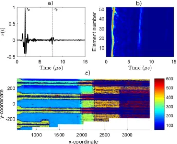
A typical ultrasound pulse is shown inFig. 1a, with two time indices marked astaandtb. These times correspond to
reflec-tions from the front and back wall of the composite panel respectively. A pulse of this kind effectively constitutes an A-scan. The information extracted from this is the time differencetf ¼tb ta, and this is often referred to as the ultrasonic TOF. This
about the attenuation of the wave as it travelled through the thickness of the plate. An A-scan thus gives information about a single physical coordinate on a surface.
A B-scan can be formed by collecting a series of A-scans along a line (illustrated inFig. 1b), while a C-scan is formed by collecting a series of B-scans, to give a two-dimensional grid of ultrasound pulse information (illustrated inFig. 1c). Note that higher times of flight inFig. 1c imply wider plate thickness. The salient features inFig. 1c are the stringers and the variable thickness of the wing panel. The purpose of the stringer is to increase the flexural stiffness in the main direction of bending. They are, therefore, characterised as thicker regions of material, typically along one direction of a plate. The stringers are evident by a low TOF index, due to their thickness being higher than the maximum value that can be captured within the collected data. These are evident as horizontal lines inFig. 1c. Immediately surrounding the stiffeners, the stringer’s feet are evident, as a reinforcement and to alleviate stress concentrations in the joint between the stringer and the main plate. The addition of layers is evident as discrete increases in TOF (implying higher material thickness).
2.2. TOF inference as a blind de-convolution problem
One way in which a greater level of physical insight could be extracted from a pulse-echo ultrasound measurement is by interpreting the measured response as a convolution process between the transducer impulse response function and the reflectivity function of the medium by which the sound is propagating[11],
xðtÞ ¼fðtÞ rðtÞ ð1Þ
wherexðtÞis the measured signal in the transducer,fðtÞis the transducer impulse response function, andrðtÞis a reflectivity function. This can be written down in discrete form as,
xðtÞ ¼X M
m¼1
fðt
s
mÞrðmÞ ð2Þwhere
s
mis a lag term. It is common to assume an impulse response function in the form of a windowed Gaussian tone burst [11]. This leads to a real-valued Gabor function, [image:4.544.99.444.54.336.2]fðh;tÞ ¼Be at2cosð
x
tþ/Þ: ð3ÞThe vectorh¼ ð
a;
x;
/Þcontains the parameters of this tone burst. Solving for the appropriatehthat best represents the mea-sured signal,xðtÞ, is a problem of de-convolution and it is an ill-posed one. It has been tackled successfully[9]using some of the sparsity tools discussed later in Section3.3. Furthermore, this model is important as it represents one way of viewing what will shortly be referred to as a dictionary, in the context of sparse coding. Some attempt by the authors has been made at treating this de-convolution problem with CS tools[12], although the present paper presents a much more general view of the problem, in which the de-convolution interpretation is just a special case. This will be more evident later in Section5where dictionary learning will be discussed.
3. Compressive sensing
The concept of CS is to circumvent the process of explicitly using a forward transform in order to compress a data set. The idea being that if the compression is done by means of random sampling (which map a highly sampled signal into a much lower-dimensional domain), the original signal can be reconstructed later on.
There are three key ingredients in CS that allow accurate signal reconstructions based on a very low number of measure-ments. The first ingredient is the assumption that the signal in question can be represented by a very low number of coef-ficients in some suitable transformation. In other words, it is sparse in that domain. This domain is represented by a dictionary. The second ingredient is the use of random transformations of the signal. It can be shown that when a signal undergoes certain random transformations, pairwise distances between measured points are preserved. This is a result of the Johnson-Lindenstrauss Lemma [13]. However, recovering this compressed version of the signal from an over-complete dictionary is an ill-posed regression problem. This is where the third and final ingredient comes into play: sparse coding, or sparse regression methods. These allow the solution of these type of ill-posed problems by assuming that most of the coefficients in the solution will be zero.
3.1. Dictionaries and the sparsity assumption
Whilst the Fourier and wavelet transforms are not the topic of this paper, they do play hidden roles in the background, and so it is worth starting with a brief discussion of sparsity and signals, with how these fit in the context of traditional Four-ier and wavelet analysis. The uninterested reader may safely skip this section. Sparsity (in the context of statistical inference) is the general idea that a dataset can be explained by a compact set of variables. In a signal processing context, this is clearly illustrated with the idea that a measurement that is dense in one domain may be sparse in another domain. A classical exam-ple in signal processing is a single sine tone; in the time domain, the data density is dictated by Nyquist theorem, but in the Fourier domain this could be accurately represented by a single (complex) number at the right frequency location. The Four-ier transform is fundamentally limited to modelling stationary (and infinite) signals. Several ideas have developed since, starting from the idea of sliding and overlapping time windows, which led to the Gabor transform, general time-frequency representations, and eventually led to the development of the wavelet transform. The wavelet transform repre-sents a signal as a combination of orthogonal wavelet functions, which are localised in time and scale, and so the transform effectively fits shifted and stretched versions of a ‘‘mother” wavelet to all time points in the signal. This is the continuous wavelet transform, and it provides the complete opposite of sparsity; it provides redundancy in the representation, as it can be evaluated at any arbitrary time and scale. An efficient wavelet representation emerged in the form of the Discrete Wavelet Transform (DWT), which discretises the mother wavelets into half-band filters (for both decomposition and recon-struction), that recursively split a signal into low and high frequency components, while decimating at every step. At this point, no sparsity is achieved in the decomposition yet, only a representation that is not redundant (the number of coeffi-cients in the representation is equal to the original measured time points). However, sparsity is only a small step away, and is in fact provided by the observation that in a discrete wavelet transform, some, and sometimes the majority of the coef-ficients can be set to zero, providing a potentially high level of signal compression. When the coefcoef-ficients are reconstructed (using the reconstruction filters of the mother wavelet), the resulting signal will only contain information encoded in those wavelet coefficients that were not switched off. This is often referred to as wavelet thresholding, and it was pioneered by Donoho[1]who also determined a simple procedure for identifying appropriate thresholds for the wavelet coefficients.
Fourier, Gabor and wavelet transforms are somewhat strict in the representations they allow. They belong to the class of completebases; they do not allow a representation of greater length than the signal itself. What if the most appropriate rep-resentation of a signal came from a combination of wavelet, Fourier or other basis? This question led to the development of over-complete bases[14–16], which pose the signal representation problem as a linear combination of basis functions,
x¼Db ð4Þ
ill-posed regression problem tractable. This problem is often referred to assparse coding, and various different algorithms have been suggested to solve it. Some of these are reviewed in Section3.3.
3.2. Random matrix projection
There is particular interest in the problem of dimensionality reduction, for the purposes of algorithm design, in a wide range of scientific disciplines; this is also central to the compression step of CS. A way of ‘‘compressing” a dataset is to project theN-dimensional measurement vectorxto a lower,M-dimensional space using a linear or nonlinear transformation. One popular approach is to use transformations, such as Principal Component Analysis (PCA), Independent Component Analysis (ICA) or factor analysis[17]. These particular examples project the measurements into spaces with certain constraints. For example, PCA is designed to rotate a data set such that the resulting vectors are forced to explain as much of the variance as possible. Such a linear transformation could be written down as,
z¼
U
x ð5Þwherezis now a low dimensional representation ofx. An interesting projection results if the rotation matrix,U, is set to be a random matrix. Johnson and Lindenstrauss[13]have shown that ifUis distributed according to a Gaussian, or Bernoulli dis-tribution, this linear dimensionality reduction preserves, with low error, certain features ofx, such as pairwise distances. A Gaussian or Bernoulli random matrix projection also yields an orthogonal transformation. This is a central result within research in metric embedding[13]. This random matrix transform is a key ingredient in the formulation of the CS problem. In this paper, the elements ofUhave been drawn from a Gaussian distribution:N ð0;1Þ, and used in order to project the orig-inal measurement vectorxinto a lower dimensions, thus compressing it.
3.3. Sparse coding
The last step in a CS scheme is to reconstruct the signal, based on the compressive measurements and a dictionary[2], which is concerned with finding a sparse set of coefficientsbthat best describe the random matrix projectionUx(the com-pressed signal representation). What is available to the regression problem is not the full signal, but rather a projection of it throughU. The coefficient set can be inferred if the basis dictionary is also projected through the sensing matrix to yield the following regression problem,
U
Db¼U
x ð6Þwhere, as before,Uis a random matrix projection,Dis a basis function set, andxis the (uncompressedn-dimensional) signal of interest.
The solution to Eq.(6), proposed in the original formulation of CS[3]is anl1regularised linear regression scheme. This
type of regression was earlier proposed in[18], in the more general context of deriving sparse solutions to ill-posed problems where sparsity can be assumed. It also goes under the name of Least absolute shrinkage and selector operator (Lasso). One of the major limitations of the Lasso is that it does not give a definite answer to the appropriate level of sparsity that represents the signal. This is due to its non-probabilistic formulation.
Common to all sparse coding schemes is the need to balance the accuracy of the solution, level of sparsity and the com-putational complexity. An optimal solution to this problem would involve checking all possible combinations of subsets ofb set to zero, and pick the one that provides the best representation of the signal. This is effectively a linear regression problem with a penalty term based on the l0 norm ofb(number of non-zero coefficients), where the following cost function is
minimised,
minimise:
1
2Njjx Dbjj
2 2þ jjbjj0
ð7Þ
However, achieving the global minimum in(7)is a non-convex, combinatorially hard optimisation problem, so an approx-imation is required in practice. A solution to this was provided by the matching pursuit algorithm[14], which is a greedy iterative algorithm for finding a sparse solution tob. Mallat originally developed MP in order to extend wavelet analysis to over-complete bases; this has already been discussed above.
While using anl0penalty would result in an optimum sparse representation, the Lasso tackles this problem by observing
that if the penalty is relaxed to anl1norm, the optimisation problem becomes convex, and thus more tractable. This is an
acceptable step because anl1penalty still encourages sparse solutions to the regression problem. The Lasso uses the
follow-ing formulation of the cost function,
minimise:
1
2Njjx Dbjj
2 2þkjjbjj1
ð8Þ
Note that thel1penalty is regularised by the termk. A generallqpenalty could be computed using the sumjjbjjq¼
PN
j¼1jbj
q,
high value ofkencourages a low number of non-zero coefficients, and vice versa. Therefore, an appropriate value ofkneeds to be chosen for each problem in particular.
The level of sparsity in the regression problem can have meaningful interpretation in physical and engineering applica-tions. This, however, will largely depend on the type of dictionary being used within the sparse coding problem. Certain dic-tionaries may force interesting solutions ofb, that can have physical interpretations. For example, in the case of ultrasound signal representation, it has been shown in[12]that the use of a Hankel dictionary built using examples of pulses, solves a de-convolution problem and thus yields the impulse response function of the system. In this case, the sparsity level is related to the number of echoes received back at the transducer, so it is clearly an important quantity to estimate correctly.
The approaches developed for solving the Lasso problem focus on providing solutions across an entire regularisation path: from high to low values ofk. The result is a transparent view of how the solution changes when different levels of sparsity are assumed. Two key algorithms for finding efficient solutions across the entire regularisation path are the Least Angle Regres-sion (LARS)[19]and one based on coordinate descent[20]. LARS solves the Lasso problem by stepping from one highly sparse solution, to another slightly less sparse solution, until all the coefficients inbare non-zero. It is particularly suited for large scale problems, but it is naturally greedy. Both coordinate descent and LARS offer efficient solutions over the entire regularisation path. When it comes to actually choosing an appropriate level of sparsity, Tibshirani suggests using cross-validation[18]. This approach works in practice, but it is computationally more expensive, and may be prohibitive in appli-cations where estimation over large quantities of data are required.
Whilst the Lasso was the sparse coding scheme used originally in the development of CS, it generally suffers from the lack of a systematic and efficient way of tuningk. Alternatives to this exist. Shortly before the development of CS, a series of algo-rithms were developed to tackle the problem of over-complete bases in Fourier, wavelet and other domains. Worth mention-ing here are basis pursuit [16] and matching pursuit [14]. The idea in matching pursuit is to start with an empty representation, check which entry inDbest matches the signal,x, add that to the active representation, and iterate over this process. As such, it is greedy and prone to finding sub-optimal solutions. Basis pursuit provides a better alternative here, since it directly solves thel1regression problem of Eq.(8), but (unlike LARS and coordinate descent) uses global optimisation
techniques to achieve this.
From the point of view of this paper, the drawback of these methods is the lack of a probabilistic interpretation; there is no quantification of uncertainty in the estimation of the parameters, and consequently in the signal reconstructions that these yield. This is the primary motivation for turning to the sparse Bayesian learning techniques developed by Tipping
[6], based on RVMs. These are discussed in Section4.
4. Sparse Bayesian learning
The sparse coding algorithms that have been discussed so far: matching pursuit, basis pursuit, Lasso, all have two major drawbacks. The first is the lack of a systematic way of dealing with uncertainty both in the measurements and in the param-eters. In other words, they are not probabilistic. The second drawback is the lack of a sound methodology for tuning the spar-sity parameter, without resorting to cross-validation. The framework of Bayesian inference is particularly well suited to deal with both of these problems. Its underlying idea is to derive a probability distribution over the parameters of the model, thus giving a measure of uncertainty in these estimates.
The particular flavour of Bayesian inference that will be used, as it is applicable to the problem of sparse coding, is the Relevance Vector Machine (RVM)[6]. This is a flexible model that can be applied to a wide range of regression and, therefore, more general signal representation problems. Owing to its Bayesian formulation, the key difference between the regression problem solved by the RVM and other (non-Bayesian) sparse coders is that it seeks a probabilistic solution for bothbandx.
4.0.1. A brief refresher on Bayesian inference
Bayes’ theorem, applied to parameter estimation, takes the usual form,
pðhjYÞ ¼pðYjhÞpðhÞ
pðYÞ ð9Þ
wherehare the unknown parameters to be estimated andYis the set of (multivariate) observed data. There are three prob-abilities on the right-hand side of Eq.(9): the prior, the likelihood and the marginal. The prior,pðhÞ, should represent a prior belief, about the process before it is observed. In sparse signal representation, this will encode the desire for a sparse solu-tion. The likelihood,pðYjhÞrepresents the distribution of the model error, with respect to the parameters. Finally, the mar-ginal,pðYÞ, can be expanded using the sum rule of probability to yield the following integral,
PðYÞ ¼ Z 1
1
pðYjhÞpðhÞdh ð10Þ
approximation paths, while Gibbs sampling and Markov Chain Monte Carlo (MCMC) methods lie in the sampling path. Whilst sampling methods may be a feasible solution to many Bayesian problems, they are not practical in the case of CS on large amounts of data. The Lasso and matching pursuit algorithms are both extremely fast if compared to a sampling-based solution. One of the main reasons the authors developed an interest in the RVM for this task is not only its Bayesian formulation, but due to the existence of a practical, fast computation for the parameters[21].
4.0.2. Formulation of the RVM
The presentation of the RVM in this paper essentially follows that of Tipping[6]. The RVM solves the following regression model,
y¼X N
i¼1
diðxÞbi: ð11Þ
The reader will recognise this as a standard regression model, where as before, the weight vector is represented by b¼½b1;. . .;bN. The basis function set is represented byDðxÞ ¼½d1;. . .;dN. An important point to note here is that in the
RVM, the basis function set is assumed to be a function of some training datax. The RVM was originally derived as a more optimal and most importantly, sparse, alternative to the Support Vector Machines (SVM) model, which solves the same prob-lem as Eq.(11), but defines the basis set as a kernel function,
di¼
j
ðx;x0Þ ð12Þwherexandx0represent two distinct points on the input space. The RVM addresses two key drawbacks of the SVM. The first
is that the basis function set,DðxÞdoes not have to satisfy Mercer’s condition. Also, unlike the SVM which selects a number of columns fromDðxÞthat scales with the number of available training data points, the RVM is designed to only select a suf-ficient and appropriate number of relevant vectors inDðxÞthat explain the observed data well, using sparsity ideas. These two key-points, underpinning the design of the RVM, are exactly what is needed in a Bayesian compressive sensing scheme: sparsity, and the ability to use arbitrary basis functionsDðxÞas long as they are both redundant and representative of the data. Note that the second requirement, ofDðxÞbeing representative of the data, is a key point here and hence why the dic-tionary has been written down as a function ofx. This is to highlight the need to somehow train the dictionary against a representative set. Whilst this notation will be dropped in the rest of the discussion, the reader should remember this point. For the benefit of the reader, a condensed summary of the RVM model is provided below, which simply follows the requirements of Bayesian regression set out in Section4.0.1above. A more complete version can be found in[6].
The observations of the model are assumed to be corrupted with noise, and this is modelled by a target vector,t,
t¼yþ
e
ð13Þwhere
e
is the noise term andyis the representation of the signal, as defined by Eq.(11). If the noise term is assumed to be Gaussian distributede
N ð0;r
2Þ, the likelihood function,pðtjb;r
2Þ, can be written down as,pðtjb;
r
2Þ ¼ ð2p
Þ N=2r
Nexp jjt yjj 2 2 2r
2( )
ð14Þ
The key ingredient, however, is the form of the prior distribution of the parameter vector,pðbj
a
Þ(wherea
is a hyperparam-eter), as it encodes one’s prior belief about the form of the coefficients. Most importantly, it is through the form of this prior that a sparse solution to the regression problem can be enforced. The RVM enforces sparsity through the use of a hierarchical Gaussian prior. This is a conjugate prior to a Gaussian distribution and thus yields algebraic forms that are tractable when multiplied by the likelihood function of Eq.(14). The form of the prior is,pðbj
a
Þ ¼Y Mi¼1
N ðbij0;
a
i1Þ: ð15ÞThe term
a
is ahyperparametervector, that defines the variance of the prior distribution of the parameters. It is formally defined asa
¼ fa
1;. . .;a
ng(wherenis the number of coefficients inb). This prior is hierarchical since a hyper-prior overthe hyperparameters also needs to be defined. This includes both the variance terms for the prior,
a
, as well as the signal noise variancer
2. Instead of setting a prior over the variance directly, a prior is set over its inverseq
¼r
2:pð
a
Þ ¼Y Mi¼1
pð
q
Þ ¼C
ðcÞ 1dca
c 1e dq ð17ÞwhereCis the Gamma function anda;bandc;dare hyperparameters of the prior and noise variance respectively (Section4.3
provides a small discussion on these). With the likelihood function of(14)and the prior of(15), the posterior distribution over the parameters can be written using Bayes’ theorem as,
pðbjt;
a;
r
2Þ ¼pðtjb;r
2Þpðbja
Þpðtj
a;
r
2Þ : ð18ÞUsing standard Gaussian identities, this yields a Gaussian distribution,
pðbjt;
a;
r
2Þ ¼ N ð
l;
RÞ ð19Þwhere the mean and variance are given by,
R¼ ðAþ
r
2D>DÞ 1 ð20Þl
¼r
2RD>t ð21ÞAis a diagonal matrix with the elements of
a
along its diagonal. Eqs.(21) and (20)define the mean and covariance of the coefficient vectorb.In order to make predictions with this model, one would wish to evaluate the distributionpðtIjt;
a
;r
2Þ(wheret
Iis a set of
testing data points), which can be shown to be a multivariate Gaussian with mean and covariance[6],
yI¼D
l
ð22ÞVI¼
r
2þD>
RD ð23Þ
The predictive mean, defined by Eq.(22), is an intuitive application of the linear transformation that defines the sparse coding problem through dictionary representation, defined earlier in Eq.(4). The predictive variance in Eq.(23)is the sum of two terms: the signal noise,
r
2and the predictive uncertainty, arising from the termD>RD. It is clearly important to derive an accurate estimate of the signal noise term as it can effectively dictate how much of the uncertainty in the prediction is governed by measurement noise, and how much of it is explained by actual predictive uncertainty against the given dic-tionary. This is effectively a problem of optimising the hyperparameters. For example, a trivial case would be to assume a very high level of measurement noise,
r
2. In this setting, the error term, given by the likelihood function of Eq.(14)wouldrender bad predictions as being within the acceptable range.
So far, the key equations of the RVM have been laid out, leading to Eqs.(22) and (23)which allow one to make a predic-tion over the mean and variance of a sparse coding problem. This leads directly to their applicapredic-tion within a CS scheme. In the sparse coding step, two aspects are missing so far, and are given in the following two subsections: the optimisation of the hyperparameter terms
r
2anda
, and the formulation of the CS problem in terms of the RVM.4.1. Hyperparameter optimisation
There are two hyperparameters that have a strong influence over the predictive distribution:
a
andr
2. A completelyBayesian approach would be to derive full posterior distributions over these, but this is not practical given that the integral resulting in the formulation ofpðb;
a
;r
2jtÞis intractable. The approach taken in[6]to solve this is to relax the requirement ofsolving for a full distribution overf
a
;r
2g, and instead optimise a point estimate. This approach is often calledtype-IImax-imum likelihood estimation, as one optimises the likelihood of the hyperparameters with respect to the data.
The problem is formulated as the maximisation of a (log) likelihood with respect to the parameters, and is given as
Lð
a
Þ ¼logpðtja;
r
2Þ ¼logZ 11
pðtjb;
r
2Þpðbj
a
Þdb ð24Þ¼ 1
2½Nlog 2
p
þ jCj þt >C 1t ð25Þ
TheCmatrix in Eq.(24)represents the covariance function of the conditional distributionpðtj
a
;r
2Þ, and is defined asC¼
r
2IþDA 1D> ð26Þ
The original RVM paper presents a procedure for finding the optimal
a
using this log likelihood based on the Expectation Maximisation (EM) algorithm. EM is an iterative algorithm that maximises the likelihood of the parameters in the presence of missing or latent variables. The algorithm (in[22]) is rather general and allows for formulation of a large class of optimi-sation problems as iterative steps between evaluations of the expectation over the hidden variables, and updates to the model parameters that guarantee an increase in the likelihood function at every step. While EM suffers from the lack of a guarantee of a global optimum solution, this can be often alleviated in practice through a good, or informed, choice of initial parameters. In the case of the RVM, however, the major drawback of the approach is that the matrix inversion required forCapplication of CS effectively reduces the value ofN, this implies a significant improvement in the computational complexity during hyperparameter optimisation (as compared to a sparse coding without compression), where repeated inversion ofC
is required. On the other hand, evaluation of the parameter covariance matrix, in Eq.(20)involves an inversion where the computational complexity scales withOðK3Þ, whereKis the number of basis functions, or columns ofD. Usually, optimisa-tion of the hyperparameters will involve evaluaoptimisa-tion of both of these quantities.
The requirement that CS places on the over-completeness ofDmakes this computational burden even worse, as it implies that the better the dictionary gets at representing a broad class of signals, the computational burden will increase in a cubic fashion. This places a limit on the number of basis vectors that are practical to use inD, in the case of sparse Bayesian learn-ing, and this goes against the requirement for over-completeness.
The EM algorithm described in[6], includes a pruning step on every iteration, where any vectordiinDthat is deemed to
be ‘‘irrelevant” is removed from the set, so the effective number of columns ofCis reduced. This pruning technique works well, but it is still a top-down approach, where the first few iterations of the algorithm will still be computationally expen-sive. Tipping himself devised a bottom-up approach in[21]where an iterative ‘‘fast” maximum likelihood estimation is pro-vided for this class of sparse Bayesian models.
A fast approach to this marginal likelihood optimisation was developed in[21], and this is the approach adopted here for the hyperparameter optimisation. The idea is to start with a single basis (column) vector,difromDand to iteratively add
and/or remove basis functions from the set of columns ofD. Some relevant criteria are required to do so in a principled sense, and in particular one that maximisesLð
a
Þ. Tipping achieves this by decomposingC(since this is the quantity of interest) into two parts, so that,C¼C iþ
a
i1d >idi: ð27Þ
Here,C idenotes the covariance matrixCwithout the contribution of theithbasis vector,di. In this form, the inverse and
determinant of the covariance can be written in the following convenient form,
jCj ¼ jC 1ijj1þ
a
1 i d> iC
1
idij ð28Þ
C 1¼C 1i C 1id
> idiC
1 i
a
iþd>iC1 idi
ð29Þ
This is helpful because it allows writing the likelihood function as the sum of the contribution ofdiand the setD i that
excludesdias[21],
Lð
a
Þ ¼Lða
iÞ þlða
iÞ ð30Þ¼Lð
a
iÞ þ12 log
a
i logða
iþsiÞ þ q2i
a
iþsi
ð31Þ
where for simplification of the above expression
si¼d>iC 1
idi ð32Þ
qi¼d > iC
1
it: ð33Þ
These two terms are referred to in[21]as sparsity and quality factors respectively. The sparsity factor can be seen as a mea-sure of how muchdioverlaps with the basis vectors already in the current model. The quality factor,qi, can be interpreted as
a measure of the discrepancy thatdiintroduces to the error of the model exclusive ofdi.
It is shown in[23]based on an analysis oflð
a
iÞthatLða
Þcan be maximised with respect toa
i, based on the followingconditions,
a
i¼ s2i q2
i si
ifq2
i >si; ð34Þ
a
i¼ 1 ifq2i 6si ð35ÞThis is an incredibly useful observation, from the point of view of sparsity and optimisation. Recall that
a
i represents theinverse variance of the prior distribution over the model weightspðbj
a
Þ. A value ofa
i¼ 1implies that the weight for basis diis infinitely peaked around zero, thus deeming it irrelevant. The iterative procedure for fast optimisation ofLða
Þdescribedin[21]therefore uses these observations in order to derive two important learning rules. For this, an ‘‘active set”Ris defined, which contains the set of vector deemed relevant. The two basic rules are:
Ifdinot in active setR, andqi2>si, addditoR.
Ifdialready inRandqi26si, removedifromR.
prioritise the deletion of basis vectors, yielding a more greedy algorithm that is computationally faster. On the other hand, favouring the addition of basis vectors would yield an algorithm that is not greedy at all in the limit of the number of func-tion evaluafunc-tions, though this may not be computafunc-tionally practical. In practice, the authors have found that accepting some level of greediness by adopting an algorithm that favours subtraction works well in practice, provided one has a reasonably good dictionary; this is further discussed in Section5.
4.2. CS formulation with the RVM
The key ingredients in the formulation of a Bayesian CS scheme have been laid out and discussed, namely random trans-formations and sparse coding, together with an efficient Bayesian formulation for sparse coding based on the RVM. This sec-tion formally defines the procedure required for reconstructing a randomly compressed signal with an RVM and provides some discussion over the issues one may encounter while applying this in practice.
So far, the RVM has been discussed in the general case of regression. Eq.(11) describes an input-output relationship betweenxandy. In the CS case, one wishes to recover the underlying true signal based on an incomplete, or compressed measurement which has been acquired through a random transformation of the original ‘‘true” signal, as described by Eq.
(5). With this in mind, the output of the basic RVM model,yin Eq.(11), can be set to the randomly transformed signal
y¼Ux, to give
Ux¼X
N
i¼1
/idiðxÞbi ð36Þ
where as before, the random transformation is given byU¼½/1;. . .;/M. Using the productUDas a dictionary, a solution for
pðbjt;
a
;r
2Þcan be found using the fast marginal likelihood optimisation procedure described in Section4.1. Eqs.(21) and(20)can be used to derive the mean and variance over the weightsb, while Eqs.(22) and (23)can be used to reconstruct the new signal.
There is an interesting point to be made regarding the evaluation of the resulting uncertainty overband ultimately over the predictions. When reconstructing a signal based on the compressed or incomplete measurementsUx, it is the product
UDthat is passed as a dictionary to the sparse coder. In the RVM, the form of the covariance for the model weightsb becomes, fromEq. (20),
R¼ ðAþ
r
2ðUDÞ>ðUDÞÞ1 ð37Þ
Considering thatAand
r
2are hyperparameters, it can be safe to say a priori, that the uncertainty inbdepends entirely onUD. The random transformationUmapsDfrom anN-dimensional ‘‘complete” space to anM-dimensional ‘‘compressed” space. Based on the Johnson-Lindenstrauss lemma, the transformationUpreserves pair-wise distances as long asMand Nstay within certain bounds. In other words, as long asMis not too low (not too much compression), then the information inDwill be well preserved inUD.
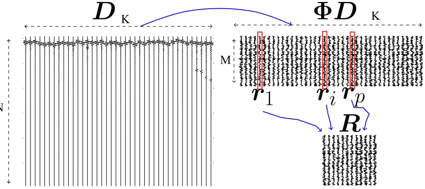
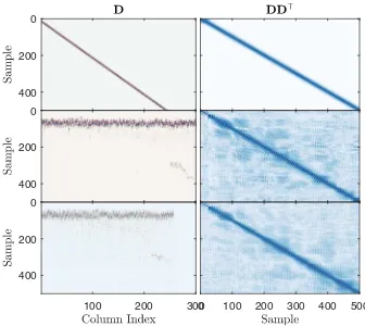
This process is visualised inFig. 2, where the map fromDtoUDtoURis illustrated. The particular dictionary used for that visualisation is a (truncated) k-means dictionary of ultrasound pulses, andUis a Gaussian random matrix. The visualisation shows that the random transform effectively shrinks the rows ofD. BecauseUDis not square any more, it is its
pseudo-D
Φ
D
R
r
1
r
i
r
p
N
K
K
[image:11.544.69.486.489.675.2]M
inverse that needs to be invertible: exactly the product in Eq.(37). As the compression level grows (lowM) so does the ‘‘aspect ratio” ofUD. If all the columns ofDwere to be kept, this matrix would be ill-conditioned at relatively highM. This is where keeping an active set,R, becomes useful. By choosing an active set of columns from the (transformed) dictionary,
UR, the RVM is basically keeping the problem invertible.
There will be a dimension below which Eq.(37)will not be suitable for inversion. However, the number of columns ofR
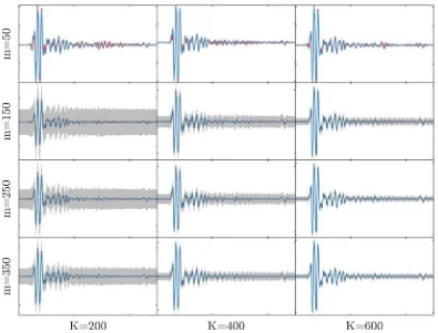
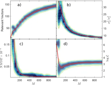
will depend on the level of sparsity of the problem; on how many relevant vectors are chosen during the hyperparameter optimisation step. Therefore, the effective level of compression will be limited by inherent level of sparsity in the signal, and how well this is represented in the dictionary. If the specific signal reconstruction problem requires a high number of columns ofUD, but there are very few rows (high compression), then only the most relevant columns will be chosen that keepURwell-conditioned (close to square). In general, ifDrepresents the data well, choosing more columns will lead to reconstructions with lower error, and vice versa. Therefore, this act of choosing an active set that keeps the problem well conditioned can be seen as adjusting the accuracy of the solution to the level of compression. It will be shown in Section6, and in particular inFig. 8that higher levels of compression results in the selection of fewer relevant vectors.
Under very high levels of compression, the inversion in(37)will not be well defined andRwill collapse. This will be illus-trated in the poor predictions of the confidence interval on the top row ofFig. 7.
4.3. Relationship between Lasso and RVM
The RVM and the Lasso could be seen as different solutions to the same underlying Bayesian linear regression problem. The RVM can be summarised as a Bayesian linear regression model that uses a hierarchical Gaussian prior in order to enforce sparsity. It is not entirely obvious how this is the case and so this will be discussed here in more detail. Sparsity is induced through the choice of a prior distribution that has most of its probability mass centred around zero. This implies that in the absence of strong evidence to the contrary (in the form of a likelihood), the weightbiwill be zero, and so the corresponding
column inDwould be deemed ‘‘irrelevant”.
The prior for the RVM is defined by Eq.(15). On its own this prior, conditioned on the hyperparameterspðbj
a
Þ, is Gaussian and does not, as such, encourage any sparsity. To see how sparsity is introduced, one has to marginalise out the weightspðbiÞ,which leads to,
pðbiÞ ¼ Z
pðbij
a
iÞpða
iÞda
i ð38Þwherepð
a
iÞis defined from Eq.(16)as a Gamma distribution. It is a fairly standard result that this integral over the productof a Gaussian and a Gamma distribution yields a Student’stdistribution. This is a key point here, because a Student’st dis-tribution with low degrees of freedom places most of its probability mass around the centre and is thus a useful sparsity-inducing prior. Recall the two sets of parameters of the Gamma distributions that describe the priors pð
a
Þandpðq
Þin Eqs.(16) and (17)respectively (a;b;candd). These control the degrees of freedom of the Student’stdistribution resulting from the integral in Eq.(38). In the case ofpða
iÞ, settinga¼b¼0 results inpða
iÞ /1=jbij, which is a prior that is sharplypeaked around zero. With low values ofaandbthe resulting Student’stdistribution will still be sharply peaked around zero, but increasing this significantly beyond one will result in the Student’stloosing its concentration of mass around the centre. In the limit of infinite values of the parameters, the Student’stbecomes a Gaussian distribution, and thus looses its sparsity-inducing characteristics. For sparsity to be induced,aandbshould be kept to as close to zero as machine precision allows. In the case ofcanddwhich control the (inverse) variance priorpð
q
Þ, their values should be kept to a small number so that its posterior is dominated by the data rather than the prior. This is common practice when doing Bayesian modelling of Gaussian distribution parameters[24].On the other hand, the Lasso is the result of a Bayesian linear regression formulation with a Laplace prior[25]. The mode of this formulation yields thel1-penalised linear regression optimisation given in(8). The issue with the Laplace prior is that
the resulting marginal likelihood is still intractable and so sampling or other approximation methods are required in order to derive the full posterior. In contrast with the Student’stprior, the Laplace distribution sets a priorpðbiÞ /expð jbijÞ. Some
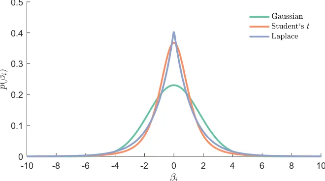
papers have been published concerning the problem of the Bayesian Lasso[26], or even Bayesian compressive sensing[27], which take the Laplace prior approach, and normally involve some form of sampling in order to get the full posterior overb. Fundamentally, the difference between the original compressive sensing formulation in terms of Lasso regression, and the one given by the RVM is the choice of prior distributions.Fig. 3illustrates this difference, comparing a Laplace, a Student’st and a Gaussian distribution. All three distributions in this comparison were generated so as to have the same variance. It is clear that, compared with a Gaussian, both the Laplace and Student’stplace most of their probability mass around the cen-tre. The Student’stdistribution is, however, much smoother than the Laplace distribution.
The application of the RVM as a sparse coding step in a CS setting has previously been carried out in[28], in an image processing context, although no application or discussion over the benefits or issues of the probabilistic interpretation is given.
5. Dictionary learning
It should be clear by now that the choice of dictionary used in any CS scheme predicates the quality of the signal esti-mates. Broadly speaking, there are two strategies for dictionaries: data-based and model-based1. The field of sparse signal
representation started, in fact, from the idea of extending traditional model-based dictionaries (such as Fourier and wavelets), to non-orthogonal, over-complete versions of these[14,16]. The idea of a model-based dictionary, however, is not restricted to signal models and can be generalised to physical models as well. In the context of ultrasound signal representation, for example, Lamb wave propagation models have been used to assemble dictionaries in a CS setting[29]. The advantage of defining a dic-tionary based on a physical, or signal model is that it only requires some broad prior assumptions about the what the signal will ‘‘look like”, without the need for measurements to be taken a priori. This does mean that for the signal reconstruction to be successful, the assumed functional forms present inDmust be roughly correct, and this is where model-based dictionaries may perform poorly.
The relevant model-based dictionary for the ultrasound examples given here is the windowed tone burst already dis-cussed in Section2.2.
If the measured signals are complex and their functional form cannot be easily summarised by simplistic mathematical formulae, creating dictionaries based on available examples of what the data might look like may be a much better strategy. This led to the development ofdictionary learningstrategies shortly after the ideas of sparse coding became available[30,31]. The use of dictionaries has already been discussed at length in the context of sparse coding for compressive sensing. How-ever, this section focusses on the specific issue of the impact that the dictionary has on the Bayesian interpretation of CS. The dictionary lies at the centre of the probability computations. In fact, it could be interpreted as defining the covariance struc-ture of the data. Recall that the covariance of a data setXcan computed using the matrix product,2
co
v
ðXÞ ¼1NXX >
ð39Þ
whereNis the number of observations. From this, it is easy to see that in order to make reasonable predictions of the uncer-tainty of the recovered signals, the structure of the productDD>should resemble that ofX
tX>t (where the subscripttdenotes
the training set). A trivial way to assemble a dictionary would be to simply setD¼Xtas this would perfectly capture the
covariance of the training data set. It is trivial because it does not summarise or decompose the structure of the data in any way. Using the training data matrix as a dictionary is also not a scalable solution since, as has already been discussed in Section4, even though the RVM scales well with low-dimensional representation, the inversion required in Eq.(20), to compute the posterior covariance, scales with orderOðN3Þ.
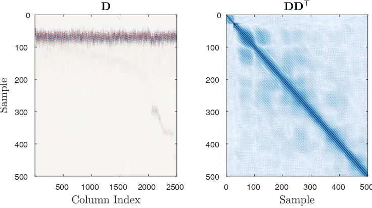
Fig. 4illustrates this trivial dictionary for a training set assembled taking 2500 ultrasound pulses at random from the C-scan data (representing a small subset of the entire data-set in this case). This will be used as an illustrative point of comparison against other dictionary types. The reader can refer back to Section1in order to readFig. 1for an example of a single ultrasound pulse, noting that (typically) there are two main reflections, from the front and a back wall. The front
-10
-8
-6
-4
-2
0
2
4
6
8
10
0
[image:13.544.110.440.57.241.2]0.1
0.2
0.3
0.4
0.5
Fig. 3.Illustration of Student’stand Laplace sparsity-inducing priors, against a Gaussian distribution. All three distributions are shown with a variance of three.
wall reflection arrives almost always at the same time, and with high energy, whilst the back wall reflection changes its arrival time depending on the local material characteristics, and is significantly attenuated. The dictionary entries (columns) inFig. 4have been sorted in ascending order of their time-of-flight (TOF) index. This is to make the visualisation of the data matrix interpretable; the columns on the left represent low TOF pulses, whilst the columns on the right represent higher TOF indices. The result is a subtle shift of the second (back-wall) pulse as the index increases. On the right,Fig. 4shows a visualisation of the covariance structure of the dictionary. This simply shows the correlation structure between the different sample indices of the signal.
Back to the dictionary learning discussion, there are two general ways in which one can force non-trivial summaries of the data: through projection or clustering. The following two sections provide an overview of dictionary learning under these two interpretations. However, the discussion will be focused around the problem of estimating good uncertainty bounds, so the respective discussions will not go into a great amount of detail.
5.1. Projection interpretation
The early developments of dictionary learning[30–32]built on the idea of using projections of the data, inspired by mod-els such as Principal Component Analysis (PCA) and Independent Component Analysis (ICA). The projection interpretation to dictionary learning uses the following generative model formulation,
x¼Dbþ
g
: ð40ÞIn this interpretation,Dis the projection matrix,bis a latent, generative variable and
g
is the noise process. PCA learns an interpretation of the model in Eq.(40)that forces the dictionary to be the set of eigenvectors of the data covariance matrix. PCA achieves this through the assumption of a Gaussian, isotropic noise process,g
, which in turn results inDbeing orthog-onal. ICA overcomes this problem by effectively allowing the modelling of non-Gaussian noise, and a non-orthogonal repre-sentation ofD. However, both PCA and ICA are in breach of the condition of over-completeness required in CS.The solution is then clearly to formulate a model that allowsDto be over-complete. To the author’s knowledge, this was first done in[30,31], by formulating the projection learning as a maximum likelihood problem with a key ingredient: enforc-ing sparsity inbby placing a Laplace priorpðbÞinside an iterative EM algorithm. This effectively adds sparse coding to the learning step, thus forcing over-complete solutions toD. Other projection-based dictionary learning strategies follow similar directions. A recent and fairly complete review of dictionary learning that covers the relevant developments up to 2011 can be found in[33].
One of the most general and complete views of dictionary learning formulated so far is the online matrix factorisation algorithm presented in[34]. A wide variety of projection algorithms can be cast as a matrix factorisation problem. A popular example would be the formulation of PCA through a Singular Value Decomposition (SVD). The ideas presented in[34]are shown to be general in the sense that minor modifications of the baseline online dictionary learning algorithm can lead to other well-known models such as sparse PCA and Non-negative Matrix Factorisation (NMF). However, the most important point in[34]is that learning is formulated as an online, or mini-batch problem. This is an important computational aspect; if the learning is sequential, only small batches of data need to be loaded into computer memory at any given time. This in turn
500 1000 1500 2000 2500 0
100
200
300
400
500
0 100 200 300 400 500 0
100
200
300
400
[image:14.544.86.454.54.260.2]500
means that learning scales gracefully to arbitrarily large quantities of data, which is crucial in applications where loading the relevant training data into memory would not only be slow, but infeasible.
The following is a summary outline of the dictionary learning algorithm of Mairal et al.[34]. Dictionary learning algo-rithms use the idea of optimisingDagainst some empirical cost function that depends on both the data and the dictionary, lðx;DÞ[31,30],
fðDÞ ¼X N
i¼1
lðxi;DÞ: ð41Þ
Here, it makes sense to definelðx;DÞas thel1regularised cost function to the sparse coding problem[35], which has already
been discussed in3.3,
lðx;DÞ,jjx Dbjj22þkjjbjj1: ð42Þ
Doing this allowsDto be over-complete, but it also means that the columnsdi, ofDcan grow to arbitrarily large values,
leading to very small values ofb. To alleviate this, the optimisation of the cost function is defined with an extra constraint, C, on thel2norm of eachdi. This allows writing down the dictionary learning as a matrix factorisation problem,
minimise:
1
2jjX Dbjj 2
2þkjjbjj1 s:tD2 C: ð43Þ
Mairal et al. arrive at an efficient iterative sequential algorithm for this optimisation using several techniques. One is the observation that minimising the expected cost,Ex½lðx;DÞ, provides computationally more efficient solutions, as stochastic
gradient optimisation schemes have high convergence rates against this expected cost[36].
The actual optimisation used is a sequential stochastic approximation that minimises a quadratic local surrogate of the expected cost. The algorithm thus splits into two steps:
1. EstimatebusingDt 1and sparse coding (whereDt 1is the previous estimate ofDduring the sequential updates).
2. UpdateDtusingb.
In this case, one assumes that observations ofxtare given sequentially at discrete time indicest. Also,D0can be initialised in
a number of ways. However, if one assumes that there truly is no prior information about the process and the data will in fact be presented to the algorithm in an online fashion, initialisation via a random matrix is a good choice for two reasons:
1. No prior information needs to be assumed.
2. Columns that remain as random vectors effectively absorb no information and can be pruned from the final dictionary.
Some readers may also notice that this update scheme is akin to the Expectation–Maximisation updates in an EM algo-rithm. In fact, there is an online generalisation of the EM algorithms that presents an alternative, but similar formulation to the same problem[37]. The key difference though is that these updates explicitly enforce a sparse solution in the ‘‘expecta-tion” step.
This algorithm can be enhanced to represent other classes of models, but for the purposes of this paper, which is to dis-cuss its applicability within a Bayesian CS framework, only the basic online dictionary algorithm has been used. Section5.3
discusses some practical aspects and results of applying this within a CS framework.
5.2. Clustering interpretation
Clustering is a particular form of unsupervised learning that seeks to summarise the density of a multivariate data-set by finding groups with certain similarities within a training set. One of the most popular clustering algorithms is k-means clus-tering, owing to its simplicity, yet sound theoretical foundations; k-means can be seen as a special case of Gaussian mixture modelling, which in turn means that there is an efficient EM formulation for a learning algorithm with certain guarantees (an increase in the likelihood of the parameters at every iteration of the algorithm).
The classical, text-book formulation of k-means clustering[38]seeks to find groups within a multivariate data setXthat minimise the Euclidean distance between every cluster centre
l
kand the (multivariate) data pointxithat belongs toK.Clus-tering is referred to as the task of finding an appropriate set of cluster centres that minimise an objective function. The task of assigning a cluster class to a data point is often referred to asvector quantisation, and is defined as,
minj:jjxi
l
jjj 22 ð44Þ
Vector quantisation seeks to represent an observationxusing the closest cluster available to it. In this sense, it is clearly a sparse coder, albeit an extreme one. The problem can even be formulated in the (now) familiar form,
where now the columns ofDcontain the cluster centres, so that for notational convenience these are redefined here as
dj¼
l
jforj¼½1;. . .;K. The coefficient vectorbis only allowed one non-zero entry, which is found using Eq.(44).It is always interesting to relate two seemingly dissimilar models as special cases of a single general model. Such is the case between projection and clustering, as pointed out by Roweis and Ghahramani[39], who explain a wide range of pro-jection, clustering, filtering and smoothing problems under the general framework of linear Gaussian models. Based on this, the obvious similarity between the projection and cluster models should not come as a strong surprise.
Similar observations have also been made regarding the similarity between the clustering and sparse coding problems
[32,40]. The specific value of k-means clustering as a dictionary learning strategy was recognised some years after the devel-opment of the projection interpretations[41,42]. In particular, Aharon[42]formulated an iterative scheme that alternates between a sparse coding step to solve forb(such as matching pursuit orl1regularised regression) and an update step of
Dbased on SVD. The method is thus called k-SVD.
For the purposes of this paper, the authors have found that the text-book k-means implementation works perfectly well in practice, and can be significantly more efficient than the k-SVD method, since efficient mini-batch and online implemen-tations exist, which are also fairly straightforward to implement.
In classical clustering analysis, one seeks to find a set of clusters that represent the data density well; that split the data into as many segments as possible, but without over-fitting. This is a crucial aspect of cluster learning. In the case of dic-tionary learning, one wishes to learn a representation that is as over-complete as possible, and over-fitting is not a real risk because the dictionary needs to be redundant. The key here is the redundancy inDrequired for a sparse solver to provide a good approximation.
What this means in practice is that if two dictionary columns,djanddiprovide equally good representations for the data,
a sparse coder will not weight equally between them, but will pick one and attempt to shrink the other as much as possible towards zero.
Even though projection and clustering can have the same formulations, the constraints applied toDare still different and thus yield different solutions. In clustering, there is no specific requirement for a decomposition of the data, whereas this may be enforced in a projection setting. In certain cases, some projections have been found to be equivalent to clustering models. For example, there is an equivalence between k-means and non-negative matrix factorisation[43].
0
200
400
0
200
400
100
200
300
0
200
400
[image:16.544.99.435.365.665.2]0
100
200
300
400
500
5.3. Effect of dictionary choice on predictive uncertainty
As already discussed, a major feature of any Bayesian formulation of a statistical model is that the predictive distribution encodes information about the uncertainty of the predictions. This section discusses the effects that the choice of dictionary form can have on the predictive distribution.
The role that the dictionary plays in quantifying the uncertainty of the predictions is evident by revisiting Eqs.(22) and (23), which define the predictive mean and covariance over the signal reconstruction, respectively. Note that the predictive variance is a sum of two terms:VI¼
r
2þD
RD>
;
r
2encodes the measurement uncertainty whileDRD>encodes theuncer-tainty in the process (how well the data relates to the dictionary).
Fig. 5illustrates three different dictionaries, derived for the ultrasound pulses discussed in Section1:
1. Model based dictionary, consisting of shifted tone-bursts. As discussed in Section2.2this leads to a deconvolution prob-lem for this specific application.
2. Clustering-based dictionary, assembled using a simple k-means algorithm.
3. Online matrix factorisation-based dictionary, derived using the algorithm in[34], and summarised above.
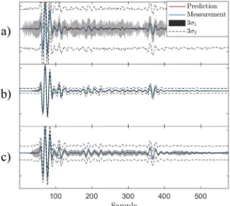
As inFig. 4, on the left is the matrixD, sorted by increasing TOF index, while on the right the productDD>is shown to illus-trate the covariance structure.3Fig. 6illustrates the difference in predictions using three different types of dictionaries. The
[image:17.544.109.438.55.350.2]greyed-out area inFig. 6shows the process uncertainty, while the dashed line denotes the confidence intervals due to full terms in Eq.(23)including measurement noise. The model-based dictionary is fairly bad at estimating the uncertainty both in terms of measurement and process noise, but has a tendency to explain most of the uncertainty as measurement noise. The simple k-means dictionary performs best in this particular example, having a tight confidence interval relating to the process noise and a small additive measurement noise term. One reason for this is that the EM algorithm, used to train EM, runs with the Fig. 6.Comparison of predictions on ultrasound data using three different dictionaries: a) model-based tone-burst, b) k-means clustering and c) online matrix factorisation. Two different uncertainty bounds are shown:r1shows predictive variance without the noise term, whilstr2shows the result of the additive noise term.
3 For visualisation purposes, the covariances have been scaled according to their diagonal variance and square-rooted. This better highlights the