Image-based tracking technique assessment and application to a fluid-structure interaction experiment

White Rose Research Online URL for this paper:

http://eprints.whiterose.ac.uk/145851/

Version: Accepted Version

Article:

Mella, D.A., Brevis, W., Higham, J.E. et al. (2 more authors) (2019) Image-based tracking

technique assessment and application to a fluid-structure interaction experiment.

Proceedings of the Institution of Mechanical Engineers Part C-Journal of Mechanical

Engineering Science. ISSN 0954-4062

https://doi.org/10.1177/0954406219853852

© 2019 The Authors. This is an author-produced version of a paper accepted for

publication in Proceedings of the Institution of Mechanical Engineers, Part C: Journal of

Mechanical Engineering Science. Uploaded in accordance with the publisher's

self-archiving policy.

[email protected] https://eprints.whiterose.ac.uk/ Reuse

Items deposited in White Rose Research Online are protected by copyright, with all rights reserved unless indicated otherwise. They may be downloaded and/or printed for private study, or other acts as permitted by national copyright laws. The publisher or other rights holders may allow further reproduction and re-use of the full text version. This is indicated by the licence information on the White Rose Research Online record for the item.

Takedown

If you consider content in White Rose Research Online to be in breach of UK law, please notify us by

For Peer Review

Image-based tracking technique

assessment and application to a

fluid-structure interaction experiment

Journal Title XX(X):1–12

c

The Author(s) 2018 Reprints and permission:

sagepub.co.uk/journalsPermissions.nav DOI: 10.1177/ToBeAssigned www.sagepub.com/

D.A. Mella

_{, W. Brevis}

_{, J.E. Higham}

_{, V. Racic}

_{and L.Susmel}

Abstract

This work analyses the accuracy and capabilities of two image-based tracking techniques related to Digital Image Correlation and the Lucas-Kanade optical flow method, with the subsequent quantification of body motion in a fluid-structure interaction experiment. A computer-controlled shaker was used as a benchmark case to create a one-dimensional oscillatory target motion. Three target frequencies were recorded. The measurements obtained with a low-cost digital camera were compared to a high precision motion tracking system. The comparison was performed under changes in image resolution, target motion, and sampling frequency. The results show that, with a correct selection of the processing parameters, both tracking techniques were able to track the main motion and frequency of the target even after a reduction of four and five times the sampling frequency and image resolution respectively. Within this good agreement, the Lucas-Kanade technique shows better accuracy under tested conditions, achieving up to 15.6% of lower tracking error. Nevertheless, the achievement of this higher accuracy is highly dependent on the position of the selected initial target point. These considerations are addressed to satisfactorily track the response of a wall-mounted cylinder subjected to a range of turbulent flows using a single camera as the measuring device.

Keywords

Accuracy assessment, Digital Image Correlation, Image-based tracking, Fluid-structure interaction, Lucas-Kanade technique

1

Introduction

The introduction of new technological advances associated to imaging devices has allowed the development of high precision and low-cost image-based techniques. In structural engineering, these techniques offer an alternative to traditional approaches such as accelerometers, strain gages, laser doppler vibrometer, among others. Their main advantages are related to the remote and non-contact nature, which can offer several benefits in cases of structures with difficult access or when simultaneous multi-point or full-field measurements are required. In general, image-based techniques use digital images to obtain displacements, geometry, or deformations of different targets [1]. In the context of engineering applications, these techniques have been used for the quantification of structural vibrations [2], damage detection [3], linear and non-linear deformations [4], crack growth during fatigue testing [5], and the characterisation of fluid-structure interactions [6,7].

Two image-based techniques frequently used in engineer-ing are based on Digital Image Correlation (DIC) and optical

flow methods. Due to their extended application in engineer-ing, this paper will focus on DIC calculated via standard Fast Fourier Transform (termed here as DIC-based technique), and the Lucas-Kanade approach (LK) [8], which is a linear approximation of the optical flow equations. Some applica-tions of the DIC-based algorithm can be found in [9], where this technique was applied on a suspension bridge to estimate the modal frequencies and tension of hanger cables subjected

1_{Department of Civil and Structural Engineering, The University of}

Sheffield, Sheffield, UK

2_{Department of Mining Engineering and Department of Hydraulics}

and Environmental Engineering, Pontifical Catholic University of Chile, Santiago, Chile

3_{National Energy Technology Laboratories, Department of Energy,}

Morgantown, West Virginia, USA

4_{Department of Civil and Environmental Engineering, Politecnico di}

Milano, Milano, Italy

Corresponding author:

D.A. Mella, Department of Civil and Structural Engineering, The University of Sheffield, Mappin Street, Sheffield, S1 3JD, UK.

Email: mvamellavivanco1@sheffield.ac.uk 1

For Peer Review

to ambient vibration loads. The difference between their results and those obtained from simultaneous accelerometer measurements was within ±_{0.5%. The response of a}

full-scale timber-framed structure subjected to synthetic seismic loads was successfully captured using DIC [10]. Their full-field measurements were validated with a Linear Variable Differential Transformer, obtaining differences of less than

5%. In the context of fluid-structure interaction, a stereo DIC-based algorithm was used to analyse differences in modal characteristics and vibrational responses of composite beams placed in different mediums [7]. Applications for the LK technique can be found in [11] for the estima-tion of the modal shapes and frequencies of a helicopter blade. The first two main modes of the structure were successfully extracted under an impulse excitation, showing good agreement with a finite element model and a classical experimental modal analysis. Amplitudes and frequencies of a targetless cable of a small pedestrian bridge has been measured using the LK technique [12]. The estimated natural frequencies were in close agreement with the spectral peak frequencies extracted from accelerometers. For the charac-terisation of a fluid-structure interaction problem, a computer vision technique based on the LK approach was used [13]. The seismic response of an underwater model subjected to three-dimensional synthetic seismic loads was successfully extracted.

Under controlled laboratory or field conditions, previous studies have validated the accuracy of the tracking techniques by comparing them to other external sensors. However, the selection of the image acquisition procedure and the parameters involved in the calculations often leads to an optimal local solution. In terms of the DIC-based technique, research on the quantification and optimisation of the variables involved in motion estimation (see, for instance, [14, 15]) indicate that there is an important dependence to the setup conditions and processing parameters. This consideration can be extended to the optical flow technique as well [16]. This work quantifies and compares the accuracy and robustness of both tracking techniques to the setup conditions and their corresponding processing parameters. Then, these results are used to measure the response of a body in a fluid-structure interaction experiment using a single recording device. For this, a high precision measurement technique and a computer controlled shaker are used to analyse the robustness and accuracy of the DIC-based and LK techniques. Their capabilities are evaluated by a comparison of the measured amplitude spectra and under changes in the tracking parameters, acquisition frequency, and image resolution. It is shown that, with proper

consideration of the experimental setup and processing parameters, both tracking techniques can satisfactorily track the target motion even after a reduction of four and five times the sampling frequency and image resolution respectively. The DIC-based technique is more robust under decrements in the image resolution. On the other hand, the LK technique is better in terms of accuracy, achieving up to 15.6% of lower tracking error in some cases. Nevertheless, this technique has an important dependency on the selection of the initial target point. This limitation is addressed through the implementation of the Forward-Backward (FB) tracking failure algorithm [17], where the response of a cylindrical obstacle subjected to different open-channel turbulent flows is successfully extracted using a single camera as the measuring device.

Nomenclature

d _{pixel displacement between frames.}d_{= [dx, dy]}

d_{ij Components of the affine transformation. i= [x,y], and} j= [x,y]

fs shaker frequency

f’

s acquisition frequency of the resampled shaker image series

fnat cylinder frequency measured in air

r cross-correlation function

sk signal k= [1,2]obtained from the tracking techniques

u _{initial target pixel coordinates.}u_{= [xo, yo]}

w _{interrogation window size.}w_{= [wx, wy]}

x _{pixel image coordinates.}x_{= [x, y]}

A _{affine transformation matrix}

D cylinder diameter

I _{first image pixel intensity values}

J _{second image pixel intensity values}

Q flow rate

N x-direction image pixel size

M y-direction image pixel size

P_{1 initial tracking point position starting from the first} image series

For Peer Review

P’

1 final tracking point position starting from the last image series

P2 final tracking point position starting from the first image series

R _{correlation map}

Re Reynolds number

RM Sn root mean square between the normalised tracking signal and CODA signals

T transpose

U bulk flow velocity

W interrogation window region

W1 interrogation window of the first image

W2 interrogation window of the second image

∆RM Sn root mean square between the difference of two signals

ǫ Lucas-Kanade technique minimisation function

F _{Fourier transform}

F∗ _{complex conjugate of the Fourier transform}

F−1

inverse Fourier transform

ν kinematic viscosity

2

Computational implementation of the

tracking techniques

2.1

Digital Image Correlation

Digital image correlation has been widely used for image processing. Particularly, this work uses the cross-correlation function to track the location of a single target. Consider two consecutive frames of equal size [N, M]. The intensity value of the first and second frame are I₍x_{) and} J₍x₎ respectively, where x_{= [x, y]}T _{corresponds to the pixel} coordinate of the frame (x= [1,2...N], y= [1,2...M]). Here, the tracking technique is applied on a region of interest called interrogation window. If an initial target pixel location u_{= [xo, yo]}T _{and an interrogation window W of size}w₌

[wx, wy]aroundu_{are selected, the discrete cross-correlation} function is given by

r(d_{) =}

u+w/2

X

x=u₋w/2

I₍x₎·₍J₍x₊d_{) (1)}

where d_{= [dx, dy]}T _{is a vector of pixel displacement} between frames (dxanddyare the pixel displacements in the xandy direction respectively). Eq.1 calculates the cross-correlation at a givend_{. If Eq.1is applied at every}d_within W, a correlation map R₍d_{) is obtained. To increase the} computational efficiency, the cross-correlation is determined in the frequency domain via a Fast Fourier Transform, where the Fourier transform of I _andJ _{are defined as}F₍I_)and

F₍J_{)respectively. The cross-correlation is expressed as}

R₍d_{) =}F−1_{F I(x)· F}∗ _J(x+d)

(2)

where F∗ _{is the complex conjugate of its Fourier} transform, and F−1

is the inverse Fourier transform. The d_{associated to the maximum value (highest peak) of}R₍d₎ corresponds to the most probable displacement of the target. An initial interrogation window W1 around the target is chosen in the first frame. A second interrogation window W2, with same size and location as W1, is placed in the next frame. Their mean intensity values are extracted to normalise image regions under uniform changes in brightness. Then, fixing the position of W1, Eq.2is applied between both interrogation windows changing d _{to cover} all pixel positions within W1. This procedure implies that the target displacement between frames is smaller than half the interrogation window size. In addition, the target displacement can be estimated within a pixel, reaching subpixel accuracy, by approximating the spatial distribution of correlations around the peak with a continuous function.

The open source library OpenPIV [18] provides the functions to obtain the position of the correlation peak with subpixel accuracy.

2.2

Optical Flow: Lucas-Kanade

The details of the LK implementation used in this study can be found in [19]. Consider two sequential frames with intensity values as I₍x_{) and} J₍x_{) respectively. Given an} initial target pixel locationu_{= [xo, yo]}T _{in the first frame,} the goal of the LK technique is to estimate its location in the second frame, [u₊d_]T_{, such as its corresponding} intensity values around the point of interest reaches a minimum difference. As in the previous section, the vector d_{= [dx, dy]}T _{corresponds to a pixel displacement between} frames. This implementation considers a square-shaped interrogation window W of size w_{= [2wx+ 1,2wy+ 1]} 1

For Peer Review

aroundu_{, and assumes that the intensity values are subjected} to the following affine transformation:

A₌

!

1 +dxx dxy dyx 1 +dyy

#

(3)

where dxx, dxy, dyx, and dyy characterise the affine deformation of the interrogation window. Approximating the intensity values of the second frame by a first order Taylor expansion series of the first frame (valid for small displacements), the objective is to find the vector of pixel displacement d _{and the affine matrix} A _{within W that} minimise the following function:

ǫ(d_,A_{) =}

u+w/2 X

x=u−w/2

I₍x₎−J₍Ax₊d₎2

(4)

Eq.4is minimised following a Newton - Rapson iteration approach. In addition, subpixel accuracy is achieved through bilinear interpolation. In case of larger displacements, [19] considers a pyramidal scheme representation.

The OpenCV library [20] contains a well-documented version of this algorithm.

3

Experimental Setup

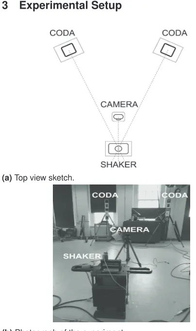
(a)Top view sketch.

(b)Photograph of the experiment.

Figure 1. Shaker recorded by a PS3 camera and a CODA system.

The experiments were performed at The University of Sheffield, United Kingdom. The APS 400 Electro-Seis shaker was used to produce a one-dimensional oscillatory, rigid motion. The amplitude and velocity of the shaker changed simultaneously to reach a particular frequency. As a consequence, a normalisation process is necessary to accurately compare across frequencies (explained later in this section).

Two systems are used to register the movement of the shaker, a three-dimensional (3D) motion tracking system called CODA CX1, used as a baseline, and a PS3 Eye recording camera (see Figure 1). The CODA system is composed of two self-calibrated 3D scanners, which track high-intensity infra-red LED markers at up to 800 Hz. The accuracy of this system in the target plane, indicated by the manufacturer, is approximately 0.05 mm when the distance between the CODA scanners and the marker is three meters. Thus, the CODA system is placed at two meters from the shaker position. The PS3 Eye camera is capable of recording 8-bit uncompressed images with a resolution of 640x480 pixels and a acquisition frequency of 75 Hz. The camera is mounted at 0.5 m from the shaker position with a field-of-view of 75 and a focal length of 2.1. These parameters produce less than 1% of distortion according to the manufacturer.

The movement of the shaker was tracked at three different shaking frequencies: 1 Hz, 3 Hz, and 4 Hz. The amplitude of the shaker for these frequencies correspond to 120.19 mm, 45.55 mm, and 25.42 mm respectively. The CODA system was set to track two-dimensional motions at 200 Hz. Simultaneously but unsynchronised, the PS3 Eye Camera recorded for 40 seconds with an acquisition frequency of 75 Hz. The discrete signals obtained by the CODA system and the ones used for the tracking techniques are subjected to the following normalisation process. Firstly, the CODA signal is sub-sampled using a spline cubic interpolation to match the sampling frequency of the PS3 Eye camera. Secondly, an equal temporal shift is applied to align the starting recording time of both systems. The shifted position is selected when the root mean square (RMS) between the CODA data and the displacements estimated by the two tracking systems reached a minimum value. Finally, both signals are normalised by their corresponding mean amplitude, followed by the subtraction of their mean positions to obtain independent coordinate signals. The mean displacement between consecutive data points of the normalised coda signal is equal to 0.056, 0.158, and 0.211 for the 1 Hz, 3 Hz, and 4 Hz respectively. The RMS between the normalised 1

For Peer Review

tracking and CODA signals, termed here asRM Sn, is used as an error measurement throughout this study.

Even though the experiments were carefully conducted to reduce perspective and lens distortions, a calibration technique was applied to further minimise these elements. In the context of small displacements (e.g. shaker amplitude is 25.42 mm at 4 Hz), these sources of error can affect the accuracy of both tracking techniques and increment their RM Snwhen they are compared to the high-precision CODA system. A calibration plate, composed by a regular grid of black circles with 3 mm diameter and 10 mm of separation, was temporally fixed on the shaker plane of motion. Then, an image of this plate was taken and used for the calibration process. A multi-quadric radial interpolation function was used to determine a transformation between the known marker distances and their corresponding pixel coordinates. Thus, undistorted real-world displacements are obtained from the original image pixel coordinates. A similar approach can be found for shallow-flow visualisations [21].

4

Sensitivity analysis

4.1

DIC-based technique: Interrogation

window size and subpixel estimation

method

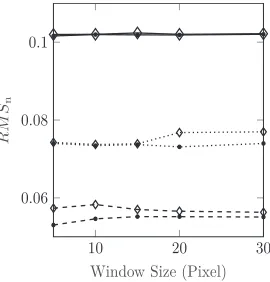
Square-shape interrogation windows with sides from 30 to 100 pixels and 10-pixel increments are investigated. The influence of the Centroid, Parabolic and Gaussian subpixel methods on the overall accuracy of the DIC-based technique are also analysed.

Fig. 2a shows the RM Sn calculated for the 4 Hz series as a function of interrogation window sizes and subpixel estimation methods. For all interrogation window sizes, the Centroid estimation method gives the highest RM Sn compared with the Gaussian and Parabolic subpixel functions. Between these last two methods, there are no significant differences in their RM Sn. The RM Sn divided by the maximum RM Sn of a given shaker frequency is shown in Fig. 2b. As [14] indicates, there is a range of interrogation window sizes that maximise the technique accuracy, which is dependent on the target displacement between frames.

4.2

Lucas-Kanade technique: Integration

window and initial target point selection

An evenly spaced squared grid of 121 initial target points with one pixel separation was placed in the shaker zone of motion. The LK technique was applied to individual

30 40 50 60 70 80 90 100 0.11

0.115 0.12

qBM/Qr aBx2 USBt2HV

R

M

SM

(a) : Centroid, : Parabolic, : Gaussian.

30 40 50 60 70 80 90 100 0

.88 0

.9 0

.92 0

.94 0

.96 0_.98 1

qBM/Qr aBx2 USBt2HV

R

M

SM

Kt

(

R

M

SM

)

(b) : 1 Hz, : 3 Hz, : 4Hz.

Figure 2. DIC sensitivity analysis. a)RM Snvs window size using different subpixel techniques b) Percentage of the maximumRM Snvs window size.

10 20 30 40

0.2 0.4 0.6 0.8

qBM/Qr aBx2 USBt2HV

R

M

SM

(a) : 90thpercentile, : 60thpercentile, : 30thpercentile.

1 25 50 75 100

0 0.2 0.4 0.6 0.8 1

:`B/ SQBMi

R

M

SM

(b) : 1 Hz, : 4 Hz

Figure 3. LK sensitivity analysis. a)RM Snvs interrogation window size (4 Hz shaker frequency). b)RM Snat different initial target points.

For Peer Review

grid points using a range of square-shape interrogation windows of sides from 5 to 40 pixels. Fig. 3a shows their corresponding RM Sn in terms of three percentiles: 30th_{, 60}th_{, and 90}th_{. For interrogation window sizes less} than 20 pixels, at least 30% of the initial target points reached the global minimum RM Sn, which corresponds to the smallest RM Sn value considering all target points. Furthermore, at 90thpercentile, theRM Sndecreases toward an optimum of 10 pixels. This optimum value is where the dependency of the LK technique on its initial target point is minimised. Outside this optimum of 10 pixels, smaller interrogation window sizes rely on a small amount of information to accurately track the movement of the shaker, which makes the tracking technique more sensitive. On the other hand, larger interrogation windows sizes produce excessive smoothing in the motion estimation and the error increases, as explained in [19]. Analysing the dependency of the LK technique on its initial target point, Fig. 3bshows all RM Sn from the 121 initial grid points at two different shaker frequencies. A suboptimal interrogation window size of 30 pixels, as shown in Fig. 3a, was used to illustrate the effects of different target displacements. Between grid points 25 to 65, a low RM Sn region is observed for both shaker frequencies. This particular region within the target corresponds to a high intensity gradient zone where the tracking technique achieves its highest accuracy. Except in a few grid points, the RM Sn decreases with the shaker frequency. Moreover, there is a higher number of target points reaching RM Sn closer to the global minimum at lower shaker frequencies. As the only experimental change was the shaker frequency, this result could be explained by the relationship between the camera exposure time and the target displacement between frames. Considering a con-stant exposure time, higher target displacements reduce the image intensity gradients and, as a consequence, lowers the tracking technique accuracy. The ratio between the 5th _and 95th _{RM Sn percentiles obtained from Fig. 3b is used to} quantify the LK accuracy regarding the initial target point selection. For the 1 Hz and 4 Hz shaker frequency, this ratio corresponds to 9.7 and 5 respectively. Furthermore, there is a high variability of theRM Snbetween consecutive nearby target points. These results indicate that the LK technique is highly dependent on the initial target point selection.

5

Changes in the operational parameters

In this section, changes in the shaker frequency, image resolution, and acquisition frequency are used to test the accuracy and capabilities of both tracking techniques. In

addition, their tracking motion estimation is analysed in the frequency domain.

5.1

Spectral analysis

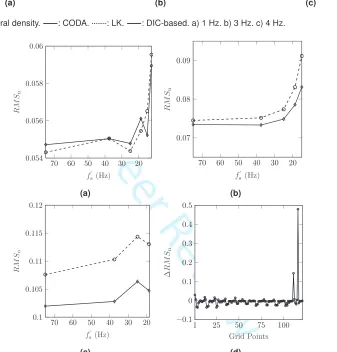
Fig.4 shows the normalised power spectral density (PSD) of the displacement obtained with the tracking techniques and CODA signals. The frequency of the shaker fs was used to normalise the spectra. The Welch method with a window size of 225 data points, and a Hamming window was used for the power spectral density calculations. In general, there is a good agreement between the tracking techniques and the CODA system. In all cases, the normalised main peak frequency is equal to 0.975, 1 and 0.995 for the 1 Hz, 3 Hz, and 4 Hz respectively. However, there are some discrepancies in the estimation of the energy contributions in the high-frequency range. Within this range, the LK technique decreases the spectral energy contribution. On the other hand, the DIC-based technique amplifies this energy contribution, producing a flat spectrum at the highest frequencies. This flatness is normally associated with the lack of performance of the measuring apparatus and tracking technique to estimate small amplitude, high-frequency displacements [22].

5.2

Acquisition frequency

Changes in the camera acquisition frequency were obtained by resampling the original time series of images. Different set of images with sampling frequencies f’

s equal to the original acquisition frequency, 75 Hz, divided by an integer factor were generated. A lower limit for this reduction is given by the sampling theorem (Nyquist criteria) to avoid aliasing effects in the signal. This limit is also constrained by the existence of enough similarities between consecutive frames, in which both tracking are able to track the target with acceptable accuracy. After a series of tests above the Nyquist frequency, it was found that the lower for the shaker motion at 1 Hz, 3 Hz, and 4 Hz, are 12.5 Hz, 15 Hz, and 18.75 Hz respectively. The acquisition frequency of the CODA signal was also resampled to match the tested sampling frequencies.

Fig. 5a, Fig. 5b, and Fig. 5c show the accuracy of the tracking techniques at different sampling frequencies. Even though both tracking techniques were able to track the shaker motion across all tested f’

s, there is an overall increment on the RM Sn as the sampling frequency decreases. As previously discussed, this could be explained by a reduction in the image intensity gradients as the target displacement between frames increases. The maximum increment in 1

For Peer Review

0 10 20 30 40

10−7

10−5

10−3

10−1

f/fb

Sa.

(a)

0 5 10

10−7 10−5 10−3 10−1 101

f /fb

Sa.

(b)

0 2 4 6 8 10

10−7

10−5

10−3

10−1

101

f/fb

Sa.

(c)

Figure 4. Power spectral density. : CODA. : LK. : DIC-based. a) 1 Hz. b) 3 Hz. c) 4 Hz.

20 30 40 50 60 70 0_.054 0_.056 0_.058 0_.06

fǶ bU>xV

R

M

SM

(a)

20 30 40 50 60 70

0.07

0.08

0.09

fǶ bU>xV

R

M

SM

(b)

20 30 40 50 60 70 0_.1 0_.105 0_.11 0_.115 0_.12

fǶ bU>xV

R

M

SM

(c)

1 25 50 75 100

−0.1

0 0.1 0.2 0.3 0.4 0.5

:`B/ SQBMib

∆

R

M

SM

(d)

Figure 5. RM Snvsf’

s. : LK, : DIC-based. a) 1 Hz. b) 3 Hz. c) 4 Hz. d)∆RM Sn, wheres1= 75Hz ands2= 18.75Hz, considering a shaker frequency of 4 Hz.

RM Snacross allf’

sis 7.9% and 12.3% for the LK and DIC-based technique respectively. On average, the LK technique shows a higher accuracy of 5.6% over the DIC-based algorithm at the highest shaker frequency. It is important to determine the influence of f’

s in the LK technique dependency to the initial target point selection. Changes of a specific parameter are assessed by introducing∆RM Sn, defined as the difference between theRM Snof two resulting

signals, s1and s2, obtained from the same initial target point, i.e:

∆RM Sn=RM Ss1

n −RM Sns2 (5)

Considering the grid described on the sensitivity analysis for the LK technique applied to the 4 Hz shaker frequency case, Fig. 5d shows the ∆RM Sn of two signals sampled at s1= 75 Hz and s2= 18.75 Hz. It is observed that decrements in f’

s do not significantly increase the LK dependency to the initial target point selection.

For Peer Review

5.3

Image resolution

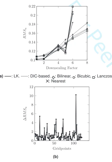
The dimensions of the original images were reduced in size up to a factor of 10 using four different interpolation techniques: nearest (the nearest pixel from the original image is used directly), bilinear (2x2 pixel window), bicubic (4x4 pixel window), and Lanczos. This last technique is a high-quality downsampling filter available in the Python Pillow library (https://pillow.readthedocs.io). Then, these low-resolution images were scaled back up to the original image dimensions using the nearest interpolation technique, which preserves their image intensity gradients. Poor tracking accuracy is achieved for the LK and DIC-based techniques when the original image resolution was reduced by a factor of six and eight respectively.

2 4 6 8

0.1 0.12 0.14 0.16 0.18 0.2 0.22

.QrMb+HBM; 6+iQ`

R

M

SM

(a) : LK. : DIC-based. : Bilinear, : Bicubic, : Lanczos, : Nearest

0 50 100

0 2 4 6 8 10 12

:`B/TQBMib

∆

R

M

SM

(b)

Figure 6. Downscaling effect. 4 Hz shaker frequency. a)RM Sn vs downscaling factor using different interpolation techniques. b)∆RM Snusings1: original set, ands2: five times downscaled.

Fig. 6a shows the RM Sn of both tracking techniques at different image resolutions. In general, the interpolation technique does not have a significant impact on the RM Sn variations at different image resolutions. There is an inverse relationship between resolution and accuracy for both tracking techniques. As the image resolution decreases, the same amount of information is contained in a lower number of pixels. As a consequence, the image intensity

gradients are reduced along with the accuracy of the tracking techniques. The DIC-based technique shows an almost linear relationship across the analysed range of image resolutions. In contrast, the LK technique does not show a clear pattern up to a downscaling of five. Then, there is a sudden increment in RM Sn for a downscaling factor of six, indicating a significant reduction in its tracking motion estimation. Considering a downsampling factor of five and the images generated using the Lanczos algorithm (lowest overall RM Sn), the LK technique has a 15.6% lowerRM Sncompared with the DIC-technique. Moreover, considering the same conditions as before, there is an increment in RM Sn of 13.4% and 20.7% for the LK and DIC-based technique respectively. From these observations, it seems that a decrement in the image resolution (i.e. loss of information) affects the tracking techniques differently. The LK technique relies on the image intensity gradients, where a lower image resolution introduces larger restrictions compared with those involved in the DIC-based technique, which relies on the target intensity patterns. Analogous to the previous section, ∆RM Sn was calculated to determine if changes in the image resolution increase the dependency of the LK technique on the initial target point selection. Selecting s1and s2, where s2was obtained from the original dataset and s2 from the images downscaled five times in resolution, Fig. 6bshows that the image resolution has an important influence on the location of the best initial target point selection.

6

Fluid-Structure Interaction experiment

In this section, the estimation of the spatio-temporal displacement of a cylinder subjected to a range of incoming turbulent flows is analysed. The comparative analysis from previous sections has shown that the LK technique is moderately better in terms of tracking accuracy, and it will be used in this section.

6.1

Experimental setup

An experiment performed at The University of Sheffield, United Kingdom, was designed to analyse the response of a slender, lightweight, wall-mounted, emerged cylinder subjected to three flow conditions. The Reynolds number is defined here as Re=U D/ν, where U is the bulk flow velocity, D is the diameter of the cylinder, and ν is the kinematic viscosity of the fluid. The tested flow conditions correspond to Re 430, 660, and 950 at a discharge rate of Q1= 0.0151 m3s−1, Q2= 0.0231 m3s−1, and Q3=

0.0355m3 s−1

respectively.Q3is also the highest possible 1

For Peer Review

discharge rate in the facility. For all tested flow conditions, the incoming turbulent intensity was 5%. The experiment was composed by a recirculating water channel covered by clear cast acrylic sheets, a cylindrical obstacle, and a recording device (see Fig.7). The flume has a longitudinal fixed slope of 0.001 m m−1

and a rectangular cross-sectional area of 486 mm width. A water depth of 347 mm was maintained using a computer-controlled system. The cylindrical obstacle was made of clear cast acrylic ofD= 5

mm diameter and a density of 1.19 g cm−3. The obstacle was tightly embedded in an acrylic sheet by fixing one end of the cylinder and leaving the other end unsupported. This arrangement allowed the cylinder to oscillate freely in both longitudinal (x-axis) and transverse (y-axis) directions. The cylinder length measured from its tip to the acrylic base was 491 mm with a natural frequencyfnatof 6.74 Hz. This value was calculated imposing an initial one-dimensional displacement on its free end. The response was recorded and tracked, obtaining a fnat closer to its theoretical value considering an Euler-Bernoulli cantilever beam behaviour.

Figure 7. Experimental setup of a cylinder subjected to an open-channel turbulent flow. Cylinder oscillations in transverse (y-axis) and longitudinal (x-axis) directions.

6.2

Tracking estimation

The maximum observable cylinder displacement for the tested flow conditions was approximately one diameter in the transverse direction. This imposes a requirement for the experimental setup, in which the transverse displacement needs to be contained within the imaged region as well as to capture the smallest longitudinal displacements with a high enough resolution. Previously, it has been shown that a lower image resolution or, likewise, an increment in the camera-object distance reduce the accuracy of both tracking techniques. Furthermore, the experimental setup presents length constraints in terms of camera mounting, available space, and object distance. As a consequence, a high-resolution MX 4M camera with a spatial resolution of

2048x2048 pixels was employed. The camera focused on a black marked circle at the free end of the cylinder. This mark generates an area with high-intensity gradients and is used as the initial tracking target. Each experiment was recorded at 8-bit and 70 Hz for two minutes. Pictures of a calibration plate, LaVision model 058-5, positioned at the cylinders free end were taken to correct for perspective and optical distortions. The calibration was performed using the software DAVIS 8.3, following a similar procedure as described in the shaker experimental setup.

As shown previously, the LK technique has a strong dependency on the selection of the initial target point. This drawback is addressed using the Forward-Backwards (FB) tracking failure technique [17]. This algorithm is based on the fact that the optical flow is independent on the direction of time, i.e. the tracking of an object from the spatial positionP_{1 to}P_{2in time is the same as between point}P₂ to P1 moving backwards in time. In practice, P1 and the final position tracked from P_{2 backwards in time, defined} as P_{1, will not be the same. Their Euclidean difference}’ is called FB-error and is a measure of the LK technique accuracy. This process is applied to a number of initial target points to identify the ones that satisfactorily represent the true motion of the target. If a cloud of initial points is considered, it is possible to select the signals whose FB-error is in the lowest 5th _{percentile. Once these signals} are identified, their corresponding mean displacement is subtracted to make them coordinate independent. At each time step, the displacement is calculated as the median value of the selected signals. Using the shaker data, Fig.8shows the comparison between the tracking motion estimation using the FB technique and the minimum RM Sn obtained on the LK sensitivity analysis section for a range of interrogation window sizes. The maximum difference across all shaker frequencies is 7.5%, showing that the FB technique effectively finds the initial target points that maximise the accuracy of the LK technique without using additional external sensors. Since the LK technique dependency is also a function of the target displacement, interrogation window sizes of 5 up to 40 pixels were tested on the recorded cylinder data. The minimum FB-error was achieved at interrogation window sizes of 10, 15, and 20 pixels. Within these options, the lower interrogation window size was selected (10 pixels) since smaller interrogation window sizes reduce the smoothing of the tracking estimation.

An example highlighting the benefits of the FB imple-mentation for the analysis of the cylinder displacements are presented Fig. 9 and Fig. 10. The values were normalised using the parameters D and fnat. A window size of 350 1

For Peer Review

10 20 30

0.06 0.08 0.1

qBM/Qr aBx2 USBt2HV

R

M

SM

Figure 8. FB with LK using the shaker images. : 1 Hz, : 3 Hz, and :4 Hz. At each shaker frequency, : min(RM Sn), and⋄:F B.

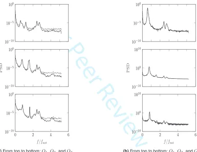
data points, and a Hamming window was considered for the Welch power spectra density calculations. In these figures, a comparison between the tracking displacements obtained implementing the FB algorithm and the tracking results that correspond to the 99th_{FB-error percentile (worst initial} target point) were performed for different Re. Significant differences in displacements and frequencies are observed. These differences are larger in the longitudinal direction, specifically in the low and high-frequency spectral range. The longitudinal response of the cylinder is up to 20 times smaller than its transverse motion. As a consequence, it is more difficult to track its longitudinal motion at a given image resolution.

7

Conclusions

This paper analyses the accuracy and robustness of the cross-correlation via Fast Fourier Transform (DIC-based) and Lucas-Kanade (LK) techniques under changes in acquisition frequency, image resolution, and internal tracking parameters. These results are then used for the quantification of body motion in a fluid-structure interaction experiment. The selection of the processing parameters of both tracking techniques plays a critical role in the estimation of the true target motion. The LK technique shows a strong dependency on the selection of the initial target point, which varies according to the target displacements and image intensity gradients. There is a range of interrogation window sizes in which the LK technique reaches its maximum accuracy. Within this range, a correct selection of the interrogation window size has the additional benefit of substantially decrease the dependency of the initial target point. On the other hand, the Parabolic and Gaussian subpixel methods of the DIC-based technique show a superior accuracy compared to the Centroid method. There is an optimum range of interrogation window sizes that

maximise the technique accuracy. With the correct selection of the tracking technique parameters, both techniques were able to track the main motion and frequency of the target even after a reduction of four and five times the sampling frequency and image resolution respectively. Considering a reduction of five times the original images resolution, the LK technique has a 15.6% lower RM Sn compared with the DIC-technique. In addition, the LK technique has, on average, a lower 5.6% RM Sn over the DIC-based algorithm at the highest tested shaker frequency and at different acquisition frequencies. Overall, the LK technique shows a superior accuracy when it is able to track the target. On the other hand, the DIC-based technique shows a higher robustness under systematic reductions in image resolution. Despite its moderately higher accuracy, the LK technique shows an important dependency on its initial target point, which difficult the achievement of its better accuracy. This dependency can be minimised through the implementation of the Forward-Backward tracking failure technique without depending on additional external sensors. These considerations were addressed in a fluid-structure interaction experiment, were the body motion of a cylindrical obstacle subjected to a range of turbulent flow was successfully extracted using a single recording device.

8

Acknowledgements

This research did not receive any specific grant from funding agencies in the public, commercial, or not-for-profit sectors.

References

[1] Baqersad J, Poozesh P, Niezrecki C et al. Photogram-metry and optical methods in structural dynamics A review. Mechanical Systems and Signal Processing 2017; 86: 17–34.

[2] Helfrick MN, Niezrecki C, Avitabile P et al. 3D digital image correlation methods for full-field vibration measurement. Mechanical Systems and Signal Processing2011; 25: 917–927.

[3] Poudel UP, Fu G and Ye J. Structural damage detection using digital video imaging technique and wavelet transformation. Journal of Sound and Vibration2005; 22: 869–895.

For Peer Review

2_.8 2_.85 2_.9

−0.2

−0.1

0 0_.1 0_.2

X/D

Y

/D

(a)

2_.5 2_.6 2_.7 2_.8

−1

−0.75

−0.5

−0.25

0

0_.25

0_.5

0_.75

1

X/D

Y

/D

(b)

2.4 2.5 2.6

−0.75

−0.5

−0.25

0 0.25 0.5 0.75

X/D

Y

/D

(c)

Figure 9. Cylinder displacement at different flow rates. Comparison between LK with the FB implementation and a LK result with a 99thFB-error percentile. : LK with FB. : 99thFB-error percentile. a)Q1. b)Q2. c)Q3

10−10

10−5

100

10−10

10−5

100

Sa.

0 2 4 6

10−10

10−5

100

f/fMi

(a)From top to bottom:Q1,Q2, andQ3

10−10

10−5

100

10−10

100 1010

Sa.

0 2 4 6

10−10

100 1010

f/fMi

(b)From top to bottom:Q1,Q2, andQ3

Figure 10. : LK with FB, : 99thFB-error percentile. a) Longitudinal spectra displacement. b) Transverse spectra displacement.

[4] Ehrhardt DA, Allen MS, Yang S et al. Full-field linear and nonlinear measurements using Continuous-Scan Laser Doppler Vibrometry and high speed Three-Dimensional Digital Image Correlation. Mechanical Systems and Signal Processing2017; 86: 82–97.

[5] Vanlanduit S, Vanherzeele J, Longo R et al. A digital image correlation method for fatigue test experiments. Optics and Lasers in Engineering2009; 47: 371–378.

[6] Huera-Huarte FJ. An optical instrument based on defocusing for dynamic response model testing in water or wind tunnels.Ocean Engineering2014; 79: 92–100.

[7] Kwon YW, Priest EM and Gordis JH. Investigation of vibrational characteristics of composite beams with fluid-structure interaction.Composite Structures2013; 105: 269–278.

[8] Lucas BD and Kanade T. An Iterative Image Registration Technique with an Application to Stereo Vision. In Proceedings of the DARPA Image Understanding Workshop 1981. pp. 121–130.

[9] Kim SW and Kim NS. Dynamic characteristics of suspension bridge hanger cables using digital image processing.NDT & E International2013; 59: 25–33. 1

For Peer Review

[10] Sieffert Y, Vieux-Champagne F, Grange S et al. Full-field measurement with a digital image correlation analysis of a shake table test on a timber-framed structure filled with stones and earth. Engineering Structures2016; 123: 451–472.

[11] Morlier J and Michon G. Virtual Vibration Measurement Using KLT Motion Tracking Algorithm. Journal of Dynamic Systems, Measurement, and

Control2010; 132: 11003–11011.

[12] Ji YF and Chang CC. Nontarget Image-Based Technique for Small Cable Vibration Measurement. Journal of Bridge Engineering2008; 13: 34–42.

[13] Rao GVR, Sreekala R, Kumar KS et al. Seismic Response Measurement of an Under-Water Model Through High Speed Camera and Feature Tracking. Experimental Techniques2016; 40: 83–90.

[14] Bornert M, Br´emand F, Doumalin P et al. Assessment of digital image correlation measurement errors: Methodology and results. Experimental Mechanics 2009; 49: 353–370.

[15] Zappa E, Mazzoleni P and Matinmanesh A. Uncer-tainty assessment of digital image correlation method in dynamic applications. Optics and Lasers in Engi-neering2014; 56: 140–151.

[16] Atcheson B, Heidrich W and Ihrke I. An evaluation of optical flow algorithms for background oriented schlieren imaging. Experiments in Fluids 2009; 46: 467–476.

[17] Kalal Z, Mikolajczyk K and Matas J. Forward-backward error: Automatic detection of tracking failures. InProceedings - International Conference on Pattern Recognition 2010. pp. 2756–2759.

[18] Taylor ZJ, Gurka R, Kopp GA et al. Long-duration time-resolved PIV to study unsteady aerodynamics. IEEE Transactions on Instrumentation and

Measure-ment2010; 59: 3262–3269.

[19] Bouguet JY. Pyramidal implementation of the affine lucas kanade feature trackerdescription of the algorithm.Intel Corporation2001; 5: 1–10.

[20] Bradski G. The OpenCV Library.Dr Dobbs Journal of Software Tools2000; 25: 120–125.

[21] Brevis W and Garc´ıa-Villalba M. Shallow-flow visu-alization analysis by proper orthogonal decomposition. Journal of Hydraulic Research2011; 49: 586–594.

[22] Bendat JS and Piersol AG. Random data: Analysis and Measurement Procedures. 4th ed. New York: John Wiley & Sons, 2011.