5-2018
Contractive Autoencoding for Hierarchical
Temporal Memory and Sparse Distributed
Representation Binding
Luke G. Boudreau
Follow this and additional works at:https://scholarworks.rit.edu/theses
This Thesis is brought to you for free and open access by RIT Scholar Works. It has been accepted for inclusion in Theses by an authorized administrator of RIT Scholar Works. For more information, please [email protected].
Recommended Citation
Representation Binding
A Thesis Submitted in Partial Fulfillment
of the Requirements for the Degree of Master of Science
in
Computer Engineering
Representation Binding
Luke G. Boudreau
Committee Approval:
Dr. Dhireesha Kudithipudi Advisor Date Professor of Computer Engineering
Dr. Ernest Fokou´e Date
Associate Professor of School of Mathematical Sciences
Dr. Raymond Ptucha Date
priorities. Felipe Petroski Such, who has shown that when you find your passion
you will pour all your energy in. Cody Tinker, who had looked beyond my
idiosyn-crasies, and continued to support me throughout my thesis. Eric Franz, for showing
me how to open doors. Dillon Graham, for insightful and intellectual discussions
regarding vector symbolic architectures, and without which a significant portion of
this research would not exist. Michael Foster and Amanda Hartung, both of which
had helped explain fundamental concepts related to Hierarchical Temporal Memory.
James Mnatzaganian, for his advice regarding the continuation of Hierarchical
Tem-poral Memory research. My Coach and his mantra of don’t think, just do, which was
a simple solution to what appeared to be difficult problems. The Rochester Institute
My Father has been an exceptional role model in my life. His experience,
perseverance, and discipline were crucial motivators for my study this field. Thank
spatiotemporal information for anomaly detection and prediction. A critical
compo-nent in the Hierarchical Temporal Memory algorithm is the Spatial Pooler, which is
responsible for processing feedforward data into sparse distributed representations.
This study addresses three fundamental research questions for Hierarchical
Tem-poral Memory algorithms. What are the metrics for understanding the semantic
con-tent of sparse distributed representations? The semantic concon-tent and relationships
between representations was visualized with uniqueness matrices and dimensionality
reduction techniques. How can spatial semantic information in images be encoded
into binary representations for the Hierarchical Temporal Memory’s Spatial Pooler?
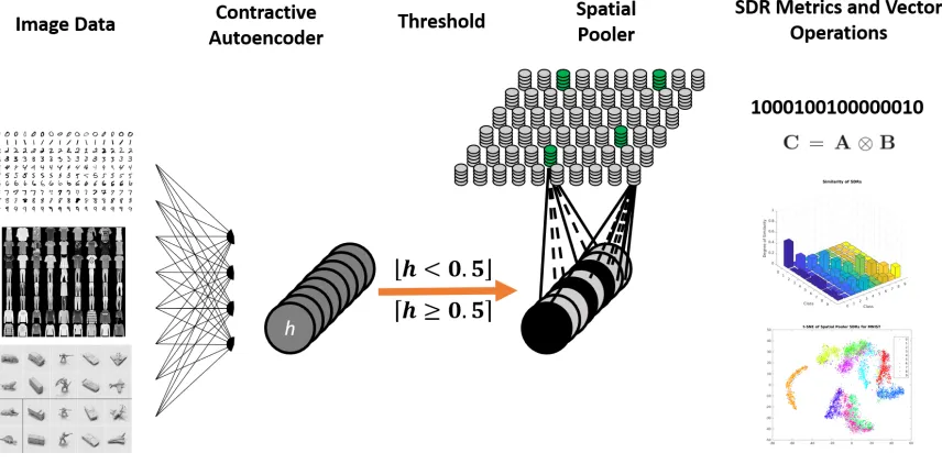
A Contractive Autoencoder was exploited to create binary representations
contain-ing spatial information from image data. The uniqueness matrix shows that the
Contractive Autoencoder encodes spatial information with strong spatial semantic
relationships. The final question is how can vector operations of sparse distributed
representations be enhanced to produce separable representations? A binding
oper-ation that results in a novel vector was implemented as a circular bit shift between
two binary vectors. Binding of labeled sparse distributed representations was shown
to create separable representations, but more robust representations are limited by
Signature Sheet i
Acknowledgments ii
Dedication iii
Abstract iv
Table of Contents v
List of Figures vii
List of Tables 1
1 Introduction 2
2 Background 6
2.1 HTM Algorithm Overview . . . 7
2.1.1 Spatial Pooler Algorithm . . . 8
2.1.2 Spatial Pooler Performance Metrics . . . 15
2.1.3 Properties of Sparse Distributed Representations . . . 16
2.1.4 Temporal Memory Algorithm . . . 18
2.1.5 Encoding Data for HTM . . . 22
2.1.6 Applications . . . 23
2.2 Vector Symbolic Architectures . . . 23
2.2.1 Binding . . . 24
2.2.2 Superposition . . . 25
2.2.3 Permutation . . . 25
2.2.4 VSA Implementations . . . 25
2.3 Representation Learning . . . 27
2.3.1 Autoencoders . . . 27
2.3.2 Sparse Autoencoders . . . 29
2.3.3 The Contractive Autoencoder . . . 30
2.3.4 Multiple Layers . . . 31
3 Research Methods 35
3.1 t-SNE and Uniqueness Matrix . . . 37
3.1.1 Measurement of Similar SDRs . . . 37
3.1.2 Visualizing the Geometry of SDRs . . . 38
3.2 CAE as an encoder for the HTM Spatial Pooler . . . 40
3.2.1 Image Datasets . . . 41
3.3 Binding of Sparse Distributed Representations . . . 43
3.3.1 Explicit Binding Operation and Spatial Pooler . . . 44
3.3.2 Creating Robust and Separable Representations for NORB . . 46
4 Results & Analysis 48 4.1 Results . . . 48
4.1.1 Spatial Pooler . . . 48
4.1.2 Contractive Autoencoder . . . 51
4.1.3 CAE & Spatial Pooler . . . 55
4.1.4 SDR Binding and Superposition . . . 58
4.1.5 Hyperparameters . . . 64
4.2 Discussion . . . 68
4.2.1 Uniqueness Metric for Semantic Similarity . . . 68
4.2.2 Contractive Autoencoder as an HTM Encoder . . . 69
4.2.3 Binding and Superposition . . . 71
2.1 The HTM Cell on the left, and a pyramidal neuron on the right. Both
have feedforward, context, and feedback connections [1]. . . 8 2.2 An example region for the Spatial Pooler. Two columns are shown
with their proximal segments. Each proximal segment contains a set of
proximal synapses (dotted and solid lines). Both columns have different
receptive fields (blue circles). Each proximal segment has six potential
synapses; connected and disconnected synapses are represented by solid
and dotted lines respectively. . . 11
2.3 The proximal segment threshold for this example is ρd = 2, and the
connected proximal synapse value is ρs = 0.5. Connected proximal
synapses are solid black lines (φ ≥ ρs), and disconnected proximal synapses are dotted lines (φ < ρs). The overlap value for the left
column is three, and the overlap for the right column is zero according
to equation (2.3). . . 13
2.4 An example of local inhibition for the second column (i = 2), where the neighborhood mask,H2, for the second column consists of the four
columns in the dotted circle. γ2 is set to the second largest overlap
value in the neighborhood because ρc = 2 according to (2.4). The
second column is considered active because it overlap value, α2 = 2 is
greater than or equal toγ2 = 2. . . 14
2.5 Learning is performed on active columns only which are represented
in green. A Hebbian learning principles governs synapse permanence
value update. The green lines illustrate the synapse permanence
val-ues that are increased by φ+, and the red dotted lines illustrate that
synapse permanence values are decreased by φ−. . . 14
2.6 The representation of the active columns after inhibition is represented
by a binary vector. The active and inactive columns are represented
in an SDR with ‘1’ and ‘0’ respectively. . . 15
2.7 Each cell can be in one of three states: deactivated (grey), active (green), predicted/depolarized (blue). . . 18
2.8 The HTM Region with active and predicted cells for Temporal Memory.
Distal segments and synapses are omitted. The region learns to predict
2.10 An under-complete autoencoder with bias terms. The reconstructed
input is represented on the right. . . 29
3.1 The encoder, Spatial Pooler, and evaluation metrics. . . 36
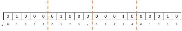
3.2 A 20 bit (N = 20) maximally sparse vector. The vector is divided into four segments (S = 4) of five bits each (L = 4). The vector is maximally sparse due to the presence of a single on bit in each segment. 45
3.3 The binding (circular convolution) of SDR A & B produce an SDR C
(C = A⊗B). All SDRs have 20 total bits (N = 20), four segments (S= 4), and five bits per segment (L= 5). . . 45
4.1 Semantic similarity between the Spatial Pooler’s SDRs for MNIST. . 50
4.2 Semantic similarity between the Spatial Pooler’s SDRs for Fashion
MNIST. . . 50
4.3 Semantic similarity between the Spatial Pooler’s SDRs for a subset of
the small NORB dataset. . . 51 4.4 Comparison of MNIST CAE reconstructions (bottom) with input
im-ages (top) . . . 52
4.5 Distribution of hidden layer activation values on MNIST dataset. There
are more saturated values with more regularization strength. . . 52
4.6 Comparison of Fashion MNIST CAE reconstructions (bottom) with
input images (top) . . . 53
4.7 Distribution of hidden layer activation values on FASHION MNIST
test dataset. There are more saturated values with more regularization
strength. . . 53 4.8 Comparison of MNIST images (top) with CAE reconstructions (bottom). 54
4.9 Comparison of Fashion MNIST images (top) with CAE reconstructions
(bottom). . . 54
4.10 Semantic similarity between the Spatial Pooler’s SDRs for MNIST. . 56
4.11 Semantic similarity between the Spatial Pooler’s SDRs for Fashion
MNIST. . . 57
4.12 Semantic similarity between the Spatial Pooler’s SDRs for a subset of
4.13 t-SNE plots of MNIST SDRs before and after binding. . . 59
4.14 t-SNE plots of MNIST before and after binding. . . 60
4.15 Membership Test of Superposition. . . 61
4.16 Membership Test of Superposition with subtractive thinning. . . 61
4.17 t-SNE plots of NORB subset at all 18 azimuths and 2 elevations. . . . 62
4.1 Spatial Pooler Parameters for MNIST . . . 64
4.2 Spatial Pooler Parameters for Fashion-MNIST . . . 64
4.3 Spatial Pooler Parameters for small-NORB . . . 65
4.4 CAE Parameters for MNIST . . . 65
4.5 Spatial Pooler Parameters for CAE MNIST . . . 65
4.6 CAE Parameters for Fashion-MNIST . . . 66
4.7 Spatial Pooler Parameters for CAE Fashion-MNIST . . . 66
4.8 CAE Parameters for small-NORB . . . 66
Introduction
Creating artificial general intelligence is a long sought goal for science, but today there
still are no machine learning systems that come close to the capabilities of the human
brain. The human brain is currently unrivaled in its ability to learn either mundane
or sophisticated tasks and has a remarkable ability to adapt to new environments and
conditions. Therefore, the human brain has been and will continue to be a source of
inspiration for artificial general intelligence development. The brain is composed of
multiple regions that are strongly integrated with each other and in some cases share
overlapping functionality. Each region is made up of a significant number of cells
called neurons; the average adult human neocortex alone contains 19 billion neurons
and around 332 trillion synapses connecting those neurons [2]. Some research assumes
that artificial general intelligence can be developed replicating the configuration of
neurons and synapses in the human brain. However, there is still not enough of a
neuroscientific understanding of the entire brain for this approach to be effective,
and the intrusive nature of gathering detailed empirical data makes it difficult to
get a complete overview of the physical structure and connections in the brain. In
addition there are significant architectural limitations associated with the design of
brain inspired silicon chips for machine learning applications. A simple neuron model
can be represented in terms of a few transistors, yet it is unclear what the adequate
IBM’s TrueNorth can model 1 million neurons with 5.4 billion transistors [3], the
configurations of neurons and synapses remain a significant problem for establishing
cognitive architectures.
A complete replication of the brain poses challenges for neuroscience with regard
to: abstraction level, computer hardware, speed of computation, and verification of
the complete system. In order to overcome these challenges, it is more effective to
analyze specific brain regions. While the entire brain is composed of interconnected
neurons and has considerable overlap in terms of functionality, it is known that certain
regions of the brain are more responsible for high level cognition than others. Studying
the brain by region reduces the scope of the problem, and provides a more scalable
approach to modeling intelligent systems.
One region of interest in the human brain is the neocortex, which is associated
with higher level intelligent behavior such as spatial reasoning, motor control, sensory
perception. The neocortex is a common region in the mammalian brain, and in the
human brain the neocortex is also responsible for language. The leading
computa-tional model of the neocortex is a theory known as Hierarchical Temporal Memory,
which establishes a memory-prediction framework that can be used for prediction,
anomaly detection, classification and sensorimotor applications. Hierarchical
Tempo-ral Memory (HTM) is a top down model in that it applies an overarching theory to
the structure and function of the neocortex [4]. HTM has been used to successfully
learn time-based sequences by using a composition of robust sparse distributed code
of cellular activations [5]. This makes HTM an effective model of sequence memory
in the neocortex. A product of this memory-prediction framework is the detection of
Robust sequence memory has helped solved anomaly detection problems, and adapts
to learn new patterns in streaming data [6]. The success of this model is dependent
on good data representations within the algorithm. The internal data representation
in HTM is known as a Sparse Distributed Representation, which contains semantic
representations of the input data. In HTM theory the Spatial Pooler is the algorithm
responsible for learning Sparse Distributed Representations of input data.
This research addresses three fundamental questions concerning HTM that focus
on the Spatial Pooler. 1. What are the metrics for measuring the quality of
semantic content for Sparse Distributed Representations? Identifying
ap-propriate criteria will help establish the correctness of data encoding techniques, and
visualize the relationships in the representational geometry of various datasets. This
will help HTM researchers analyze the content of Sparse Distributed Representations
without assuming or focusing on producing separable representations that are sought
in classification tasks.
2. How can spatial semantic information in images be encoded into
binary representations for the Hierarchical Temporal Memory’s Spatial
Pooler? Image data contains many features such as object locations, orientation,
shading, lighting, shadows, edges, and color. The relationships between these feature
are extracted and untangled in the visual cortex for high level understanding. In
HTM it is unclear what is the ideal level of features that should be passed to the
Spatial Pooler, and how they should be encoded to preserve the important
relation-ships among the image for the desired application. The added constraint for this
problem is that these features and their semantic relationships must be encoded in a
binary format, so regardless of how abstract or specific the feature space is it must be
represented in a binary format for compatibility with the Spatial Pooler algorithm.
This work examines the effect of the encoder on the semantic relationships found in
of representations. Vector Symbolic Architectures make use of a binding operation
to create robust and complex representational structures. An implementation of a
binding operation is explored for HTM’s Sparse Distributed Representations, and the
effect of the binding operation on the representational geometry is illustrated with
dimensionality reduction techniques. In addition this work demonstrates the
effective-ness of binding and superimposing Sparse Distributed Representations to create more
robust representations. A small investigation will also explore the density increase of
the vectors after superposition, which has a significant impact for manipulation and
Background
This research begins by looking at the brain as a source of inspiration for intelligence.
A crucial area of interest in the brain is the mammalian neocortex because it
respon-sible for many high level brain functions such as sensory perception, cognition, motor
commands, spatial reasoning, and language. The neocortex is considered crucial to
higher level cognition, and understanding how the neocortex gives rise to high level
cognition is done by examining how it is constructed. Neuroscientists have
discov-ered a uniform arrangement of pyramidal neurons in the neocortex. The pyramidal
neuron’s arrangement and intrinsic connectivity is found in six stacked layers that
is commonly referred to as a cortical column. The neocortex is a sheet of cortical
tissue that is composed of adjacent and repeated cortical columns. All regions in the
neocortex function on the same principles regardless of the function of the region.
The regions for vision, hearing, touch, and language are composed of the same
re-peated cortical columns [4]. The neocortex is flat by nature for some mammals such
as rodents, but in humans the neocortex is much larger and highly folded onto itself.
The same fundamental cortical column exists in different mammals’ neocortex, so the
use of the fundamental cortical column is likely responsible for high level cognition.
The modeling of the cortical column begins at the cellular level, and requires
a more robust or biologically accurate neuron model than other artificial neurons.
nections of the artificial and neocortical pyramidal neurons are shown in Figure 2.1.
Hierarchical Temporal Memory (HTM) proposes a theory or model of how
informa-tion is processed in the neocortex with a focus on explaining how the cortical column
functions. The repetition of the cortical column and the uniformity of the neocortex
is one of the guiding principles for HTM theory, and the understanding of a cortical
column will likely give insight into how the entire neocortex operates regardless of
the information domain. This theory requires a more biologically accurate neuron
model then common artificial neurons. Because of this HTM is a biologically
influ-enced and constrained machine intelligence algorithm. A major challenge of HTM
theory is the incorporation of new neuroscience research, which results in changes
and enhancements to the algorithm to ensure its accuracy in modeling the cortical
column.
2.1
HTM Algorithm Overview
The biological constraints in HTM are based on the uniformity and repetition of
pyramidal neurons found in layers 2/3 of the neocortex. In HTM theory pyramidal
neurons are referred to as the HTM neuron orcells. Cells are stacked intocolumn in
layers 2/3, and a collection of these columns form an HTMregion. The region models
the structure and functionality of the cortical column in the neocortex. The cells in a
region receive information from three different sources; feedforward, contextual, and
feedback information is transmitted through three different connections as shown in
Figure 2.1. The connections to cells are referred to as segments, and each segment is
composed of a set ofsynapses. Information flows to cells by means of synapses, and in
active, inactive, or predicted. The state of each cell is induced by the information
it receives. The processing of feedforward input is done by algorithm called the
SpatialPooler, and the processing of feedforward and contextual input is done by
algorithm called Temporal Memory. The feedback connections are not addressed
[image:20.612.237.408.196.321.2]because current HTM theory suggests that feedback is an optional component [7].
Figure 2.1: The HTM Cell on the left, and a pyramidal neuron on the right. Both have
feedforward, context, and feedback connections [1].
2.1.1 Spatial Pooler Algorithm
The Spatial Pooler is an unsupervised machine learning algorithm that converts
bi-nary input into a bibi-nary Sparse Distributed Representation. The purpose of the
Spatial Pooler is to continually encode streams of binary sensory data into Sparse
Distributed Representations, while at the same time ensuring that a generalized
repre-sentation is produced for similar inputs. A Sparse Distributed Reprerepre-sentation (SDR)
is generated by processing the feedforward input to cells in the HTM region.
In the Spatial Pooler there is no connectivity between cells; each cell only
re-ceives information fromproximal segments. Inter-cellular connectivity is described in
section Section 2.1.4, when the Spatial Pooler is combined with other components
of HTM theory. The proximal segments transmit the same information to all cells
in a particular column. The proximal segment contains a set of potential proximal
de-thanθwill be unconnected. The typical value used for the threshold of connectivity is
0.5, so only permanence values greater than or equal to 0.5 will result in a connected
synapse. The synapses are learned connections, and is inevitable that throughout
learning some synapses will be connected and some will be disconnected based on the
permanence value.
The initialization of the Spatial Pooler is done by establishing the all the column’s
proximal segment’s connectivity to the input space. Each column’s proximal segment
has potential connections to only a fraction of the input space. Each column in the
re-gion has a receptive field, which is a subrere-gion of the entire input space. The synapses
in the column’s segment connect to only a fraction of the possible inputs in the
re-ceptive field. The organization of the column’s rere-ceptive fields to the input space is
known as topology. An example receptive field is shown in Figure 2.2. Topology is
useful when there is some natural ordering or spatial relationship among the input
space [1]. A possible method to implement topology is to have neighboring column’s
receptive fields overlap, which gives the opportunity for neighboring columns to
po-tentially receive the same input. The lack of topology indicates that the receptive
fields are global with respect to the input space. In this case the receptive field for
each column is the entire input space, and the proximal synapses can potentially be
connected to any input variable. With or without topology, the permanence values
of each synapse in a proximal segment is randomly initialized. This leads to synapses
that are both connected and disconnected to the input space.
After Initialization, the Spatial Pooler can process and learn from input data.
Cells in the Spatial Pooler become active when there is enough input to the
same proximal segment, in the Spatial Pooler all cells become active together.
How-ever, there are scenarios where one cell or only a portion of cells within a column
become active due to feedforawrd input, and scenarios where cells enter the
depo-larized or predicted state. These phenomena occur when the Spatial Pooler is used
other components of HTM theory, which is explained in Section 2.1.4. The remainder
of this section will consider that the cells within column share the same state, and
the possibility of these states are eitheractive orinactive. The presence of any active
cells in a column indicate that the column is active, i.e. a column is considered active
if there are any active cells within the column.
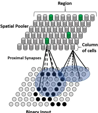
Columns of cells with proximal segments are shown in Figure 2.2, this diagram
illustrates the structure of the Spatial Pooler with feedforward connections. The level
of column activation is known as theoverlap value, and if the value is below a certain
thresholdθstimthen the column has an overlap value of 0. Overlap values are inhibited
in a global or local manner to determine which columns (and consequently the cells
within) remain active. Inhibition is used to introduce sparseness in the resulting active
column population. Global inhibition sets top k column’s with the largest overlap
values to active. Local inhibition establishes neighborhoods of columns, and selects
columns with the top k% overlaps to be active within their neighborhoods. In either
case the targeted column activation density is strictly 2% for global inhibition, and
it’s approximately 2% for local inhibition [1]. When topology is implemented in the
Spatial Pooler, then local inhibition takes into consideration the spatial relationships
among the input space.
After inhibition, the output of the Spatial Pooler is a set of columns with active
cells. However, the active columns can be represented as a binary vector or SDR,
this is the learned representation of the input. An example SDR is shown set of
column/cell activations can be represented by a binary vector as shown in Figure 2.6.
Figure 2.2: An example region for the Spatial Pooler. Two columns are shown with their proximal segments. Each proximal segment contains a set of proximal synapses (dotted and solid lines). Both columns have different receptive fields (blue circles). Each proximal segment has six potential synapses; connected and disconnected synapses are represented by solid and dotted lines respectively.
synapses based on the surviving active columns. Only proximal synapses connected
to active columns are updated by a Hebbian learning mechanism: the permanence
values of synapses that have an active input are strengthened, but the permanence
value of synapses with inactive input are weakened.
The Spatial Pooler behavior can be described as a three step algorithm that
in-volves an activation calculation for each column, a non-linear inhibition process, and
a Hebbian learning step. The mathematical formalization of the Spatial Pooler
algo-rithm presented in this work is attributed to [8]. Examples for all three steps in the
Spatial Pooler algorithm are illustrated: Figure 2.3 shows overlap step, Figure 2.4
shows the inhibition step, and Figure 2.5 shows the learning step.
1. Overlap This stage determines a set of active cells/columns given an input
sample. A column is considered active if there are enough active and connected
synapses. A connected synapse is one where its permanence value is greater
are represented by Φ ∈ [0,1]mxq, where m is the number of columns in the
region and q is the number of proximal synapses per column. The input space
is represented byXmxq. An active synapse is one where the input to the synapse
is a binary value of ’1’. The column overlap is the sum of all the active and
connected synapses belonging to the column’s proximal segment, and can be
computed using the dot product or matrix multiplication (2.2). The index
i ∈ [0, m) in (2.2) and (2.3) identify the specific columns. The calculation is performed for each column in the region denoted by (2.2), which produces a
vector of overlap values for all the columns α~ˆ ∈ Z1xm. If the column overlap
value is larger than the proximal segment threshold, ρd, then the column is
active otherwise it is inactive (2.3). In some implementations of the Spatial
Pooler, a mechanism called boosting is used to encourage columns with few
historical activations to become active. This value is represented by an overlap
coefficient ~bi in 2.3; different methods for the calculation of a column’s boost
value are explored in [8][1]. Figure 2.3 shows the overlap computation of two
columns with different proximal segments. The result of this stage is a set of
all active column overlap values, and is defined asα~ ∈Z1xm.
Y ≡I(Φ≥ρs) (2.1)
~ˆ
αi ≡Xi•Yi (2.2)
~ α≡ ~ˆ
αi~bi α~ˆi ≥ρd,
0 else
∀i (2.3)
Figure 2.3: The proximal segment threshold for this example isρd= 2, and the connected
proximal synapse value is ρs = 0.5. Connected proximal synapses are solid black lines
(φ ≥ ρs), and disconnected proximal synapses are dotted lines (φ < ρs). The overlap
value for the left column is three, and the overlap for the right column is zero according to equation (2.3).
active columns that will form the SDR. The two types of inhibition are global
and local inhibition. In either method a column’s neighbors are determined
by its neighborhood mask, Hi, which is an element-wise multiplication with
the set of active columns from the previous step (2.4). In the case of global
inhibition the neighborhood mask is the entire region (all columns within the
region), so each column effectively uses the same neighborhood mask. In (2.4)ρc
determines the level of sparsity, and is typically defined around 2% of the total
number of columns in the region [9][8][1]. The kmax(x, k) operation picks the
kth largest value from x. The kth max overlap value for the specific column iis
known asγi, which is calculated in (2.4). The k-max values,γiare used to inhibit
the set of active columns, ~α, based on the overlap values (2.5). The result of
this step is a set of active columns or a sparse distributed representation, which
is represented by the binary vector~c.
~
γi ≡max(kmax(Hi~α, ρc),1)∀i (2.4)
~ˆc≡I(α~
i ≥γ~i)∀i (2.5)
3. Learning The final step is a form of Hebbian learning. Learning is only
inhibi-Figure 2.4: An example of local inhibition for the second column (i = 2), where the neighborhood mask, H2, for the second column consists of the four columns in the dotted
circle. γ2 is set to the second largest overlap value in the neighborhood because ρc = 2
according to (2.4). The second column is considered active because it overlap value,α2 = 2
is greater than or equal toγ2 = 2.
tion step. The synapse permanence values are scalar weights between 0 and
1. The synapses with active inputs have their permanence values increased,
and synapses with inactive inputs have their permanence decreased. The
up-date values for all active columns are determined by equation (2.6). Inactive
column’s proximal synapses remain unaffected. The learning rate is controlled
by the parameters φ+ and φ− (increment and decrement values). The
appli-cation of the update is shown in equation (2.7), and ensures that the synapse
permanence values stay between 0 and 1.
δΦ≡~cˆT (φ+X−(φ−X¯)) (2.6)
Φ≡clip(Φ⊕δΦ,0,1) (2.7)
Figure 2.5: Learning is performed on active columns only which are represented in green. A Hebbian learning principles governs synapse permanence value update. The green lines illustrate the synapse permanence values that are increased byφ+, and the red dotted lines
[image:26.612.258.388.72.145.2]Figure 2.6: The representation of the active columns after inhibition is represented by a binary vector. The active and inactive columns are represented in an SDR with ‘1’ and ‘0’ respectively.
2.1.2 Spatial Pooler Performance Metrics
There are four metrics for evaluating Spatial Pooler performance based on the
in-puts and outin-puts [1]. These metrics can help establish when the Spatial Pooler has
finished learning from the given data and rate of learning for the Spatial Pooler. It
also provides information about column utilization and sparseness, which is used to
evaluate the robustness of the SDRs.
1. Sparseness The sparseness of the Spatial Pooler is the percentage of active
columns at a particular time step. This metric can be used to determine the
sparsity of the inputs to the Spatial Pooler as well as the number of columns
utilized. This metric is typically used to observe the sparsity of columns when
local inhibition is utilized.
2. Entropy The entropy is the average activation frequency of each mini-column,
and determines if the Spatial Pooler is actively using every column efficiently.
This metric determines if all the columns in the region are being utilized equally,
so the entropy effectively evaluates the distributed degree of the representation.
3. Noise RobustnessThe measurement of sensitivity to random bit flips ensures
that the Spatial Pooler is resilient to noise. The more noise required in the input
to substantially change the output SDR, the more robust the representations
4. Stability Stability ensures that the active columns remain consistent when
there is no changes to the input stream. This metric measures the degree to
which the Spatial Pooler is learning; a low stability value means that the Spatial
Pooler is actively learning from new samples, and a high stability value can be
interpreted that the Spatial Pooler has not learned new spatial patterns since
the last stability measurement.
2.1.3 Properties of Sparse Distributed Representations
It was shown that the active columns in an HTM region can be represented by a
Sparse Distributed Representation as shown in Figure 2.6. The benefits for
repre-senting data in this as a binary sparse distributed representation is robustness to
noise, effective measure of similarity between representations, and bitwise operations
for manipulation.
The distributed nature of the representation ensure that the semantic meaning is
distributed over the entire vector, for a single element in a distributed representation
does not have significant meaning related to the whole representation. This creates
robustness if a bit is not encoded correctly or is prone to noise, but most of this
resiliency is only found with high dimensional SDRs greater than or equal to 2048
bits or columns [10]. As a consequence the dimensionality governs the total number
of columns and cells within an HTM region. The use of an HTM region should be
sufficiently large to gain the robustness benefits. The sparse nature of the
represen-tations is imposed from the Spatial Pooler inhibition process. The typical targeted
values of sparseness are around 2%, which results in about 2% of the bits in the SDR
are active depending on the type of inhibition used [1].
The distributed representation found in SDRs is contrasted with a localist
repre-sentation; a single computing element represents a single entity in a local
able memory, automatic generalization, and the selection of the rule that best fits
the current situation [11]. This claim can be summarized in that distributed
repre-sentations are more adequate for models of memory structure and processing in the
brain.
Because the SDR is a binary vector it is trivial to calculate the degree of similarity
between two SDRs, which can be computed with a sum of logical AND operations.
However, it can also be computed by taking the dot product between two SDR vectors.
Numenta calls this measure of similarity SDR overlap [10]. Computing similarity or
dissimilarity is important when combined with the union property of SDRs. The union
property allows a set of SDRs to be composed into a single SDR or union of SDRs.
The union SDR contains an unordered set of SDRs that were superimposed together
by taking the logical OR operation between all SDR vectors. The determination
of set membership is done by computing the SDR overlap (dot product) between a
the union SDR and a known SDR, and if the value of the similarity is above some
threshold, θ, then that known SDR is considered a part of the set. There is a limit
to how many vectors can be stored in a set because as the number of vectors in the
union increases the false positive rate for membership increases as well [10].
In context of HTM the SDRs represent the active columns in the Spatial Pooler,
and more specifically the SDR represents the semantic information and relationships
in the feedforward input. However, in the broader context of HTM research and the
neocortex an SDR is considered to be the state of any cortical neuron population. In
the Temporal Memory portion of HTM as described in Section 2.1.4, the set of active
cells and predicted cells are each considered SDRs. The properties described in this
the use of SDRwill refer to the set of active columns that is generated by the Spatial
Pooler.
2.1.4 Temporal Memory Algorithm
The processing of feedforward and contextual input for pyramidal neurons in the
neocortex is modeled by the Temporal Memory algorithm in HTM theory. The
Spa-tial Pooler is always utilized with Temporal Memory, but there modifications to the
Spatial Pooler algorithm. The input to the Spatial Pooler is now treated as
spatio-temporal data, so the ordering of spatial input has contextual meaning. The
con-textual data is stored at the cellular level; different cell activations within the same
column in a region represent the same spatial data in different contexts. The
con-textual data shown in Figure 2.1 received from other cells within the Region. The
transmission of contextual data between cells is done through distal segments, where
a distal segment is activated through cell activations. Each cell has several distal
segments, and if the cell receives enough activity on any of its distal segments, the
cell enters the predicted state. The possible cell states for Temporal Memory and the
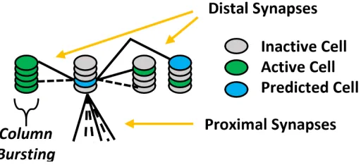
[image:30.612.198.454.483.600.2]proximal and distal synapses are shown in Figure 2.7.
Figure 2.7: Each cell can be in one of three states: deactivated (grey), active (green), predicted/depolarized (blue).
All cells in the same column correspond to the same spatial data, but different
col-Spatial Pooler algorithm selects are particular column for activation, then a
phenom-ena calledbustingoccurs. The column bursts by activating all cells within the column.
The cell with the least distal segments within the column is selected to establish a
new distal segment. The connectivity of the distal synapses in the new distal segment
is determined by the cells that were activated in the previous time step. This is done
to learn the new temporal patterns in the spatial data. Because HTM is a continuous
[image:31.612.197.454.314.512.2]online learning system, it adapts to changes in the data it processes.
Figure 2.8: The HTM Region with active and predicted cells for Temporal Memory. Distal
segments and synapses are omitted. The region learns to predict changes in input data.
The formalization of sequence memory was defined in [5], and is annotated here
for completeness. The set of active cells for a given time step is stored inAt which is
indexed throughicells andj columns. The calculation of active cells,At, requires the
active columns that were selected by the Spatial Pooler. TheWtvector represents the
indices of the active columns or bits in SDR produced by the Spatial Pooler algorithm
are selected to be active within an active column, which is described by the first case
in (2.8). If there are no predicted cells within the column then the column bursts.
All cells within the bursted column are put into the active state, which is described
by the second case in (2.8).
aij =
1 if j ∈Wt and πijt−1 = 1
1 if j ∈Wt and P iπ
t−1 ij = 0
0 else
(2.8)
The set of predicted cells for an input is given by Πtwhereπ
ij is the ith cell of the jth column. Cells are predicted if there is any segment that has an activation value
greater than some threshold θ (2.9). The predicted cells, Πt, are determined based
on the current active cells, At, calculated in (2.8). A set of distal synapses form a
distal segment, and each cell can have many distal segments. The distal segments and
synapses represented by aDd
ij matrix where the weight is stored in the dth segment’s
connection to theith cell of the jth column. Every cell has a distinctDd
ij matrix with
values [0,1]. When the Dd
ij is used in (2.9) the synapse permanences are rounded to
binary values, which is denoted by the ˜Ddij matrix.
πij =
1 if ∃dkD˜dij ◦Atk1 > θ
0 else
(2.9)
The learning or adjustment of the synapse permanence values only occur on
ments that correctly predicted cells from the previous time step (2.10). These
seg-ments are those that caused the prediction of cells that were subsequently active in
the next time step.
segment across all cells for the winning columns ofWt(2.11). The most active segment
is determined by computing the dot product between the synapse permanence values
and the previously active cells. Because there was not enough activity or the synapses
were unconnected, the weights are mapped to binary values ˙Dijd. The binary values
are calculated based on the nonzero and zero entries inDijd, the segment that produces
the largest cell activation is the candidate for learning.
∀j∈Wt(
X
i
πijt−1 = 0) and kD˙dij ◦At−1k1 =
maxi(kD˙dij ◦A t−1k
1)
(2.11)
The learning rule for selected segments in (2.11) is a form of Hebbian learning
rule on synapses (2.12).
∆Ddij =p+( ˙Dijd ◦At−1)−p−D˙dij (2.12)
There is a small decay applied to those distal segments that induced cell
predic-tions where cells did not become active in the subsequent time step. These segments
responsible for incorrect predictions have a small decrement across all permanence
values (2.13).
∆Ddij =p−−D˙ijd where atij = 0
and kD˜dij◦At−1k1 > θ
2.1.4.1 Initialization of distal segments and synapses
The initialization of the distal segments is not clear according to [5] as (2.11) does
not explain how theDd
ij connections are formed. In [6] a greedy approach was used to
establish distal segments from the current activated cells,At, to the previous activated
cells At−1. In this manner a history of previous cell activations was required to keep
track of where to initialize distal segments.
2.1.5 Encoding Data for HTM
Data must be converted to a binary representation of pred in order to be used for
input to the Spatial Pooler. In cases where data is not binary an encoder must be
used to convert the data to an SDR. Numenta has proposed several types of encoders
for encoding scalar data and spatial data [12]. After encoding, similar semantic input
should have overlapping active bits in their SDRs after being encoded. The encoder
has a strong influence on what aspects of the data contribute to the similarity.
Numenta has proposed a formalization for the encoding process in their encoding
work [12]. This formalization considers an arbitrary space A and S(n, k) an SDR
with n total bits and k active bits where f is a function of A → S(n, k). In order to evaluate the encoder, a distance metrics over space A is established in equation
(2.14). The performance of the encoder can be evaluated by comparing the distances
scores of pairs of inputs with the overlaps of their encoding. Equation (2.15) shows
that encodings with more overlapping bits have greater semantic similarity.
dA :A×A→R
∀x, y ∈A, dA(x, y)≥0
∀x, y ∈A, dA(x, y) =dA(y, x)
∀x∈A, dA(x, x) = 0
2.1.6 Applications
The SDRs in HTM can be used for traditional classification problems, but the
tempo-ral memory is more strongly used for prediction and anomaly detection tasks. HTM
does not currently explain how long term memory is recalled and stored, so an
exter-nal classifier is required for practical application tasks. Common exterexter-nal classifiers
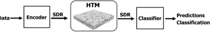
[image:35.612.158.499.295.350.2]used are SVM or softmax [8][1].
Figure 2.9: High level architecture for an HTM learning system. Because memory and
recollection is not well understood in the neocortex, the SDRs must be passed to a classifier for classification of input. An SVM or Softmax layer are typically used for classification problems.
2.2
Vector Symbolic Architectures
Jackendoff proposed four challenges for cognitive neuroscience related to the
under-standing of grammer in language in 2002 because traditional connectionist models fail
to address symbolic processing that is necessary for language [13][14]. Most
impor-tantly these challenges are not exclusive to language, but are central to higher level
cognition. The main issue with connectionist models is the lack of symbolic structure
based representations, and the construction of complex thoughts or sentences from
basic thoughts or words [15]. Jackendoff’s first problem for cognitive neuroscience is
the binding problem, which applies to vision as well as language. An example of the
each object presenting different features/attributes such as a red square and a blue
circle. In this scene, how does the brain associate red with square and blue with circle
and not vice versa? These issues were presented in the form of challenges by Ray
Jackendoff. In response, Ross Gaylor proposed a connection based model that
an-swered Jackendoff’s questions , and coined the term “Vector Symbolic Architecture”
[14].
The central element in Vector Symbolic Architecture (VSA) is the vector
repre-sentations, which can have different restrictions depending on the architecture. The
difference in these representations leads to different implementations of the basic
vector operations. The differences in VSA implementations are further described
in section Section 2.2.4 alongside descriptions of the vector operations. There are
common representations
The distributed vectors in VSA implementations are designed for powerful
recur-sive binding operations that are necessary for the processing of simple and complex
concepts [16]. In addition to variable creation, the binding operation can be used
to create novel concepts and content addressable memory structures. Content
ad-dressable memory functions is a type of memory system where the the content of the
representations is used to traverse through memory. This approach to memory design
is similar to how memory in the brain works, and is unlike the memory paradigm that
has driven classical computation [11]. The binding problem has been posed in other
contexts, and it has been suggested that binding in the brain is crucial for weaving
temporal information into signals [17].
2.2.1 Binding
In the context of VSAs there are thematic relations or roles that are associated with
some attribute or filler. The role and filler vectors are bound (or associated) together
dimension-of representations ensures that all structures (either basic or complex) have a
consis-tent time complexity for all operations, and establishes an upper memory limit for
the storage of vectors. The composition of the bound vectors is unique relative to
both composites [14]. The binding operation is invertible allowing for the recollection
of either of the composing vectors given the other, which allows for the recollection
of memory.
2.2.2 Superposition
More complex structures can be created by superimposing vectors into a single
vec-tor. The composition vectors could be bound attribute-value pairs of vectors, and
the superposition would be a collection of these role-filler pairs. Unlike the binding
operation, the superposition operation preserves the similarity between its elements.
2.2.3 Permutation
According to Kanerva, the permutation operation is versatile operation in for binary
vectors [18]. An advanced use of the permutation operation is to implement a thinning
technique for binary vectors [19].
2.2.4 VSA Implementations
There are various implementations of Vector Symbolic Architectures, and each
imple-mentation comes with advantages and disadvantages. These impleimple-mentations differ
in the choice of values used for the vector representations and size of vectors, which
in turn lead to different implementations of vector operations. A common theme
providing a binding mechanism, but the method in which the outer product
reduc-tion occurs differs. The implementareduc-tions listed here are not meant to be exhaustive,
but to illustrate the different approaches to implementations of VSA theory.
All VSAs provide a solution for the representation of sequences/recursive/tree
structures [20] associations of items may be the subject of other associations. The
reduction must be reversible, so that expansion can be done in both directions [20].
2.2.4.1 MAP
Ross Gayler proposed Multiply, Addition, Permutation (MAP) as VSA symbolic
ar-chitecture as a direct solution to Jackendoff’s challenges. Gayler discusses how to
generate vectors for novel concepts, which is crucial for adding to existing structures
or analogical reasoning [21].
2.2.4.2 Holographic Reduced Representations
Tony Plate proposed using circular convolutions to construct associations of vectors
without increasing the dimensionality of the bound vector. Since vectors are bound
using circular convolution and are unbound using circular correlation, these memories
are coined holographic [20].
2.2.4.3 Binary Spatter Codes & Hyperdimensional Computing
Pentii Kanerva’s approach to Vector symbolic architectures is to create high-dimensional
binary vectors, which were born out of a model for long term memory called Sparse
Distributed Memory [22]. The operations here utilize bitwise operations for binding,
representations for data is crucial for the application of learning algorithms. In HTM
theory there are simple encoders for low dimensional data, which creates a need to
explore other methods of encoding data into robust representations. The continuous
online learning nature of HTM systems conflicts with neural networks that extract
features based on labeled data (Alexnet,VGG-16,Resnet), so instead unsupervised
representation learning systems are more in line with HTM theory. Autoencoders
have provided a way to learn hidden representations by learning to reconstruct input
in an unsupervised manner (no class labels). It has been shown that initializing a
deep neural network with a trained autoencoders weights on the same data dataset
improves performance of the deep neural networks.
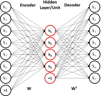
2.3.1 Autoencoders
The Autoencoder network is an unsupervised machine learning architecture that
learns to form efficient codes for input data. A single autoencoder is composed of two
layers: the encoding layer and decoding layer, or encoder and decoder. The encoding
layer transforms the input into the encoded representation (hidden units), and the
decoding layer transforms the encoded representation back into the input domain.
Hidden unit activations are computed with the encoder, which is typically a linear
combination of the input and the encoder’s weights followed by a non-linear
acti-vation function (2.16). The decoding layer is a linear combination of the decoder’s
weights and the encoded representation (hidden units) (2.17).The learning of these
encoded representations (or hidden unit activations) is guided by how well it is able
to reconstruct the input data. Learning of the weights and biases is accomplished
error. The reconstruction cost is defined as a squared error between the input and
reconstructed input (2.18).
fθ(X) =h =σ(W X+b) (2.16)
gθ(h) =σ(W X+b) (2.17)
J(θ) = X
t
L(x, gθ(f)) (2.18)
There are several variations of the autoencoder with many tunable
hyperparame-ters. For example the lack of activation functions for both the encoder and decoder
allow the network to learns a similar subspace as Principle Component Analysis [23].
However, the lack of non-linear activation functions in the autoencoder do not allow
for layers to be stacked to create “deep” networks. Regularization of the weights
can also be applied to the autoencoder to prevent over-fitting on the dataset, which
becomes an issue when the number of hidden units approaches or exceeds the
dimen-sionality of the input data. In many cases the l2 regularization term is applied to the
autoencoder’s cost function, but another form of regularization that is used are tied
weights. Tying the weights of the encoder and decoder (WD = (WE)T) means that
the weights of the encoding layer and decoding layer are identical but transposed.
Traditional applications of the autoencoder include dimensionality reduction
be-cause the dimension of the encoded representation could be smaller than the input
space dimensionality. Another usage scenario is to train the autoencoder on a labeled
dataset, and use the weights of the autoencoder to initialize the weights of a
mul-tilayer perceptron network. This approach to initialization has helped improve the
Figure 2.10: An under-complete autoencoder with bias terms. The reconstructed input is represented on the right.
2.3.2 Sparse Autoencoders
Another form of regularization that is applied to autoencoders is enforcing sparsity
in the hidden unit activations; sparse regularization will drive many of hidden unit
activation values to zero, and will enforce very few nonzero activation values. The
reg-ularization term is added to the reconstructed cost to create the overall cost function.
Two commonly used sparse activation terms are the student-t and Kullback-Leibler
divergence. Sparse autoencoders trained on natural image patches learn edges that
2.3.3 The Contractive Autoencoder
The Contractive Autoencoder (CAE) was proposed in 2011 by Rifai et. al as way
to learn robust representations [25]. This autoencoder implementation includes a
regularization penalty on hidden unit activations. The regularization term is the
Frobenius norm of the Jacobian weight matrix (2.19). The analytic penalty is
min-imized with low-valued first order derivatives, which leads to the notion of flatness
or contraction as described by the authors. This penalty encourages training data
to be lie on a relatively low-dimensional manifold in the high dimensional feature
space by contracting the input data in the directions of small variations. These small
variations in the input are captured by the autoencoder because it helps differentiate
the reconstruction of neighboring training examples.
kJf(x)k2F =X
ij
∂hj(x) ∂xi 2 = dh X i=1
(hi(1−hi))2
dx
X
j=1
Wij2 (2.19)
The encoder utilizes a non-linear activation (sigmoid), which constrains the hidden
layer activations to values between zero and one. The decoder has no activation
function (linear transformation), or in some cases a sigmoid activation function is
used. The full autoencoder is shown in (2.20), which combines the encoder and
decoder together for the reconstruction y of x (input). According to Rifai et al,
tied weights are used in the CAE to avoid scaling and expansion in the encoder
and decoder respectively. This ensures that the weights (learned features) allow the
transformation to a flat manifold, but also provide the capability to reconstruct the
input space. Tied weights also avoid degenerate solutions [23].
y=WTσ(W x+bh) +by (2.20)
The CAE minimizes its regularization term by ensuring that the derivative is
Hessian in addition to the Jacobian [26].
2.3.4 Multiple Layers
Multiple layers can be realized with autoencoders to learn more invariant relationships
in the data. As long as non-linear activation functions exist between layers, then
subsequent layers will learn non-linear transformations. However, the connectivity
and loss functions become more complex as more layers are introduced. Subsequent
layers can be implemented as a reconstruction of the previous layer’s hidden units,
or there can be several encoding layers followed by several decoding layers.
2.4
t-distributed stochastic neighbor embedding
Visualizing the structure and shape of high-dimensional data is an critical problem
that exists in many domains, and there are several techniques for representing
high-dimensional in lower dimensions. One of these methods is t-distributed stochastic
neighbor embedding, which is a nonlinear dimensionality reduction technique that
can reduce data to two or three dimensions [27]. The t-distributed stochastic neighbor
embedding (t-SNE) algorithm is capable of capturing the local structure of data quite
well. However, t-SNE is also prone to misinterpretations that arise with different
values of hyperparameters [28].
Two of the main hyperparmeters are the number of steps in the algorithm and
the perplexity. The perplexity is a smooth measure of the number of neighbors each
point has, and should be smaller than the total number of points in the dataset.
2.5
Memory in the Neocortex
Because of the invasive nature of measuring and difficulty recording neuron activity
at the necessary granularity, it is difficult to study, locate, and isolate specific or
individual memories in the brain. There are many theories of how stimulus is encoded
in the brain, yet there is no major evidence that one of these encoding mechanisms
drive all others. Population encoding finds meaning in a population of neurons in a
defined region of the brain. A population of neurons can be modeled with a vector
of values; each value in the vector represents the activation strength of a neuron. In
the extreme case the values of the vector could be represented with binary values,
which abstractly indicates if the neuron is active with no information regarding the
strength of the activation. When looking at a several thousand neurons or a vector
with thousands of elements this space becomes high-dimensional. The individual
elements of these vectors do not have specific meaning, but the meaning of the vector
as a whole contains information about where the vectors lies in the high-dimensional
space.
While it is commonly accepted that there are many categories of memory in the
brain (short-term, long-term, implicit, explicit), it has been difficult to identify the
physical mechanisms in the brain that drive the creation, recognition, and
recollec-tion of these memories. Two types of memories crucial to high level cognirecollec-tion are
semantic and episodic. It is widely accepted that semantic memories are stored in
the neocortex, which are likely encoded in a distributed populations of neurons [29].
2.5.1 Semantic Memories
An individual’s knowledge of the world is based on acquired facts: concept attributes,
concept behavior, interactions between individuals, the meaning and relationships
many data modalities to achieve a thorough understanding of the world.
There are two approaches for evaluating semantic memory according: there is the
study of semantic memory structure and the recall of semantic memory. Experiments
that study the structure of semantic memory are not concerned with accuracy of
the the semantic memories, and instead these experiments rely only on the subjects
output. However, experiments that study the recollection of semantic memories do
evaluate the accuracy, and subjects time for recollection are recorded.
2.5.2 Episodic Memories
It is important to provide a contrast to explain what semantic memory is not; episodic
memory is autobiographical memory that is unique to personal experience. An
episodic memory is encoded in a temporal relationship to other episodic memories,
and each episodic memory contains many semantic facts. Episodic memories are
rela-tive to the individual experience, and are autobiographical in nature. While episodic
memory is thought to arise in the Hippocampus, the Neocortex plays a role by
pro-viding semantic information for the construction of an episode [31]. The Neocortex
is responsible for the consolidation or binding of episodic memories into distributed
circuit for long-term storage [32].
Most AI systems today do not make use of episodic memories. The relationship
between semantic and episodic memory is coupled, but the relationship is mostly one
way. Semantic memory can operate independently of episodic memory with a few
2.6
Representation Similarity Analysis
A known challenge in Neuroscience is the mapping of computational models of neural
circuits to physical brain-activity. Techniques for acquiring empirical brain-activity
include fMRI, scalp electrophysiology EEG, MEG, all of these methods provide
differ-ent granularity. Scalp electrophysiology can record the electrical activity of individual
cells, whereas fMRI measures the hemodynamics of brain regions. Activity overlap
is expected in both cases, but it is difficult to establish a one-to-one mapping of the
different scales and data modalities. The same problem arises again when trying
to find mappings between computational models and empirical data from the brain.
A solution to this mapping problem is Representational Similarity Analysis, which
focuses on the comparing only the similarity of data in each unique domain [33].
The characteristic metric in Representational Similarity Analysis (RSA) is the
Representational Dissimilarity Matrix. The Representational Dissimilarity Matrix
(RDM) is a symmetrical matrix containing a measure of dissimilarity between activity
patterns. Each cell in the matrix corresponds to the level of dissimilarity (similarity
when inverted?) between all activity pattern pairs for two given stimulus. The matrix
is symmetrical along a diagonal of zeros in an ideal case. The measure of distance or
The first research question,What are the metrics for measuring the quality of
semantic content for Sparse Distributed Representations?, was addressed
with a uniqueness matrix and t-SNE plots. Both these methods focus on the semantic
content of Sparse Distributed Representations (SDRs) in HTM. The uniqueness
ma-trix is an extension of Mnatzaganian’s uniqueness metric for SDRs, which establishes
a specific value for the similarity between any two SDRs. The second evaluation
technique, t-SNE, was used for visualizations of any semantic clusters in the SDR
data. A comparison between the uniqueness matrix and the t-SNE techniques was
implemented throughout all experiments to show the tradeoffs between the two
visu-alization techniques.
The second research question, How can spatial semantic information in
images be encoded into binary representations for the Hierarchical
Tem-poral Memory’s Spatial Pooler?, was addressed by the use of the Contractive
Autoencoder as an encoder for HTM. The Contractive Autoencoder (CAE) was
eval-uated for its capability to extract spatial semantic information in images and its
compatibility with the HTM Spatial Pooler. The CAE was used to extract image
features from grayscale images on the MNIST, Fashion-MNIST, and small NORB
datasets. The performance of this encoding technique was compared with the
were determined experimentally by using the uniqueness matrix and t-SNE plots to
analyze the Spatial Pooler SDRs.
The third research question, How can vector operations of Sparse
Dis-tributed Representations be enhanced to produce separable
representa-tions?, was addressed by the implementation of an SDR binding operation. The
binding operation was inspired by neuroscientific theory describing interaction
be-tween the neocortex and hippocampus, and also inspired by the binding operation
in Vector Symbolic Architectures. The binding operation was demonstrated on the
MNIST dataset for separability. The binding operation was also demonstrated with
the small NORB dataset by superimposing a set of bound SDRs together. This
was done to demonstrate how more complex SDRs might be created from simpler
SDRs. In addition a small exploration was done to study the density of SDRs for
superimposition.
The overall system architecture with the Contractive Autoencoder, Spatial Pooler,
[image:48.612.111.539.436.647.2]Evaluation Metrics, and vector operations are shown in Figure 3.1.
useful for gaining insight into raw datasets, debugging representations in machine
learning algorithms, and providing intuition for preprocessing. Applying
dimension-ality reduction techniques to HTM systems will provide this insight into the structure
of the raw dataset, the structure of the data after it is encoded into a binary
rep-resentation, and the structure of the Spatial Pooler’s SDRs. There are two types of
dimensionality reduction techniques: those that preserve local structure and those
that preserve global structure. This work uses t-SNE [27] for the visualization of
the global structures of raw data, encoded data, and SDRs. Because t-SNE is an
optimization process, convergence is influenced by the hyperparameters. The effect
of these hyperparameters can have a drastic effect on the visualization and
repro-ducibility [28].
3.1.1 Measurement of Similar SDRs
The computation of similarity (SDR overlap) can be computed by taking the dot
product of two SDRs. Mnatzaganian’s work on Spatial Pooler proposed a novel
metric based on SDR similarity for evaluating the similarity of the representations
[36]. The similarity value or overlap metric, mu, indicates the degree of similarity
for a set of SDRs. This value is computed by taking the average overlap value and
dividing it by the maximum overlap (3.3). The average overlap for a set ofn SDRs is
computed by (3.1), and the maximum overlap is computed by (3.2). A µ value of 1
indicates that all the SDRs are identical and a value of0 indicates that all the SDRs
are unique.
ao= 2
Pn−2 s=0(
Pn−1
u=s+1(Ws•Wu))
mo=kmax m−1
X
i=0
Ws,i∀s,2 !
(3.2)
µo =
ao
max(mo,1) (3.3)
This work utilizes the uniqueness metric to construct a uniqueness matrix for
datasets with class labels. The process for constructing the uniqueness matrix is
dependent on labeled data, which is used to compute c(c− 1) uniqueness metrics for all possible pairs of SDRs for two classes. In (3.2) W is defined as the union of
SDRs from two classes. The uniqueness matrix displays information about the global
structure of data by illustrating the similarity between different classes. In addition
it also displays information concerning the local structure of the data. The local
structure is shown by the diagonal in similarity matrix, indicating how similar SDRs
within the same class appear. Because of all the possible c(c−1) class pairs, the matrix is symmetrical along the diagonal axis.
3.1.2 Visualizing the Geometry of SDRs
It is important to observe the effects vector operations on SDR geometry that
oc-cur when SDRs are bound and superimposed together. If the geometry of the SDRs
change due to vector operations, then the data clusters of the points may change as
a result. While methods like t-SNE or UMAP are state of the art for global
struc-ture [37], the visualizations rely on a preconceived notation of neighboring points
or number of classes (perplexity parameter for t-SNE and k-nearest neighbors
algo-rithm for UMAP). However, the neighboring number of points may change as the
representational structures (SDRs in this case) are manipulated by vector operations,
so methods that capture the geometry without a preconceived notion for the shape
![Figure 2.1: The HTM Cell on the left, and a pyramidal neuron on the right. Both havefeedforward, context, and feedback connections [1].](https://thumb-us.123doks.com/thumbv2/123dok_us/63797.6012/20.612.237.408.196.321/figure-cell-pyramidal-neuron-havefeedforward-context-feedback-connections.webp)