Some problems in stochastic models for epidemics

by

R. Dunst a n

A thesis submitted to the Australian National University

for the degree of Doctor of Philosophy

Department of Statistics Research School of Social Sciences

Canberra February 1981

The material in this thesis is my own original work except where specific reference is made.

A C K N O W L E D G E M E N T S

The work in this thesis was carried out in the Department of Statistics

(IAS) at the Australian National University. My financial support was

provided by the Federal Government of Australia in the form of a

Commonwealth Postgraduate Scholarship and by a supplement to this scholarship

provided by the Australian National University. To these bodies I extend my

thanks.

I especially wish to thank my supervisor Dr D.J. Daley for his help at all stages in the preparation of this thesis, in particular for always being ready to set aside his work when I wished to see him, for many interesting

and invaluable discussions, and for his friendly and cheerful nature. I

also wish to thank Professor P.A.P. Moran for his kindly willingness to be

of any assistance. My thanks go to all the members of the Department for

providing a relaxed and pleasant atmosphere in which to work.

I am indebted also to Dr A.J. Dobson for her help during my earliest attempts at research at the University of Newcastle, and to the Division of Mathematics and Statistics of the CSIRO in Canberra where I had a short but rewarding visit before beginning my studies at ANU.

T AB L E OF C O N T E N T S

ACKNOWLEDGEMENTS .. ... (ii)

PREFACE ... ... (v)

CHAPTER 1: INTRODUCTION ... 1

1.0 Introduction ... 1

1.1 The model ... 2

1.2 The distribution of the final size ... 5

1.3 The distribution of the time to extinction . . . . 7

1.4 The stochastic threshold theorem ... 9

1.5 A quasi-deterministic approximation ... 11

1.6 The application of the general epidemic model to r u m o u r s ... 12

1.7 The general epidemic in a stratified population .. 15

CHAPTER 2: THEORETICAL RESULTS ON THE GENERAL STOCHASTIC EPIDEMIC M O D E L ... 18

2.0 Introduction... 18

2.1 The state probabilities ... 19

2.2 The mean final s i z e ... 21

2.3 The second moment of the final s i z e ... 25

2.4 The moments conditional on a major outbreak . . . . 28

2.5 The distribution of the final size ... 29

2.6 The probability of early extinction ... 31

2.7 The mean duration time ... .. 32

2.8 The general epidemic model with a latent period before infectiousness .. .. „... 33

2.9 The birth and death process limit ... 37

2.10 The diffusion limit ... 0... 40

CHAPTER 3: APPROXIMATING PROCESSES .. . . 42

3.0 Introduction... 42

3.1 A quasi-deterministic model ... 42

3.2 The approximating process .. ... 46

CHAPTER 4 : THE GENERATION-WISE SPREAD OF INFECTION ... 56

4 . 0 I n t r o d u c t i o n ... 56

4 C1 The m ean g e n e r a t i o n s i z e ... 56

4 . 2 An a p p r o x i m a t i n g p r o c e s s ... 52

4 . 3 A l i m i t i n g p r o c e s s ... .. . . . . ... 65

CHAPTER 5: THE GENERAL EPIDEMIC IN A STRATIFIED POPULATION . . . . 67

5 e 0 I n t r o d u c t i o n ... 67

5 . 1 The t h r e s h o l d t h e o r e m ... 68

5 . 2 The p r o b a b i l i t y o f e a r l y e x t i n c t i o n ... 71

5 . 3 The p r o b a b i l i t y t h a t i n i t i a l i n f e c t i o n d o e s n o t s p r e a d ... 72

5 . 4 The f i n a l s i z e s ... 74

5 . 5 E x p e c t e d t i m e t o e x t i n c t i o n ... 76

5 . 6 An a p p r o x i m a t i n g p r o c e s s ... 77

5 . 7 The d i f f u s i o n l i m i t ... 81

CHAPTER 6 : SOME OTHER MODELS FOR EPIDEMICS ... 83

6 . 0 I n t r o d u c t i o n ... 83

6 . 1 A m o d e l f o r a n e p i d e m i c i n a c o m m u n i t y w i t h v e r y r e s t r i c t e d m o b i l i t y ... 83

6 . 2 A t w o - t y p e b r a n c h i n g p r o c e s s m o d e l ... 87

6 . 3 A m o d e l f o r a n e p i d e m i c i n a s t r a t i f i e d p o p u l a t i o n . 94 APPENDIX A: P r o o f o f T h e o r e m 2 . 1 ... .. . . . . 102

APPENDIX B: C o m p a r i s o n o f t h e g e n e r a l s t o c h a s t i c e p i d e m i c m o d e l t o a p p r o x i m a t i o n s ... ' 107

APPENDIX C: A p p l i c a t i o n o f t h e q u a s i - d e t e r m i n i s t i c a p p r o x i m a t i o n t o t h e p r e d a t o r - p r e y m o d e l 0 . . . ... 120

APPENDIX D: The j o i n t p . g . f . o f t h e n u m b e r o f b i r t h s i n e a c h s u b p o p u l a t i o n i n a l i n e a r m u l t i v a r i a t e b i r t h a n d d e a t h p r o c e s s ... 126

PREFACE

With the exception of the final chapter, this thesis is concerned with the general epidemic model and some simple extensions of it. The main concern is with the stochastic case and the deterministic model is only of interest when it is useful in constructing approximations to the stochastic model or in providing insights into its behaviour.

The model itself is quite old, appearing first in a paper by Kermack and McKendrick (1927). It is the simplest of stochastic models incorporating the two features:

(i) the rate of spread of infection is a function of the number of infectives and susceptibles present; and

(ii) infectives may be removed from the process (corresponding to death, isolation or recovery with immunity).

These two features must be regarded as essential for any model which would hope to describe realistically the spread of infectious disease.

Despite its conceptual simplicity, the model presents enormous

mathematical difficulties which we believe have not yet been successfully overcome and this has severely limited an analysis of its strengths and weaknesses in potential applications to real data. This is a very unhappy

situation as such a model is merely the beginning of a satisfactory

mathematical theory. We have attempted to solve some of these difficulties both by obtaining what theoretical results we could and by utilizing

methods leading to approximations where theoretical results were either unobtainable or whose complexity rendered them useless.

previous researchers. For instance the approximating model presented in chapter 3 arises by combining in a new way ideas of Kendall (1956) and Faddy (1978), resulting in a technique which gives good approximations for all the mathematical quantities of interest and which may be applied to the various extensions of the model which are discussed in later chapters.

However, with the exception of chapter 1 which presents a brief survey of results needed for later work, and with a few exceptions where indicated, the material in this thesis is to the best of my knowledge original.

The remaining paragraphs of this preface are a brief summary of the contents of the thesis.

Chapter 2 presents some results of a theoretical nature on the general stochastic epidemic model. Solutions for the joint probability generating function (p.g.f.) of the stochastic variables of the general epidemic model were first found simultaneously by Gani and Siskind (1965). Each used a

transform technique and the solution obtained was in a recursive form and extremely complicated. More recently, Billard (1973) obtained a solution in simpler form using matrix methods. Since the process is a finite Markov chain in continuous time and such processes may be described by a linear differential equation

p(t) = i4p(t) ,

Because of the Markovian structure of the process renewal-type

arguments may be applied in many situations. For instance, simple recursive expressions may be obtained for the expected final size of the epidemic and for its expected duration time. These two examples are known results, however we have used this technique to deal with the second moments of the

final size (in this chapter) and with various quantities arising in

extensions of the model (in chapters 4 and 5). By purely algebraic methods we are able to use these recursive expressions for the moments of the final size to find their asymptotic series expansions as the population size becomes large. The expansions throw light on the behaviour of the process, particularly when its bimodal nature is taken into account. These

asymptotic results will be published in a paper to appear in the Journal of

Applied Probability in 1980. We have also been able to apply this algebraic

technique to the probability of complete infection of the population and to the probability of early extinction of the epidemic. While in this first case the proof is incomplete, computer calculations indicate the correctness of the conjecture. Heuristic reasoning based on these asymptotic results leads to a simple technique giving the asymptotic form of the mean duration time of the process.

Because we wish to use this same heuristic technique, as an aside in this chapter we discuss briefly an extension of the model to include a non­ zero latent period between an individual’s becoming infected and becoming infectious.

The second comes simply from the application of a result of Barbour (1974). The result is of interest mainly because of its usefulness in an application in chapter 3.

The form of the solution obtained in chapter 2 is still too complicated to allow its use except for very small population sizes. The material in chapter 3 is largely concerned with developing and evaluating an

approximating process. Faddy (1977) found that by replacing a stochastic variable in one of the two transition probability rates by its deterministic

equivalent, the resulting process became a member of a general class of compartment models for which a simple solution was available. However, numerical results given by Faddy showed that the error introduced by the resulting loss of randomness was most apparent as a change in the initial behaviour of the process. We were able to rectify this by combining this

idea with Kendall’s (1956) explanation of the bimodal nature of the general epidemic process«

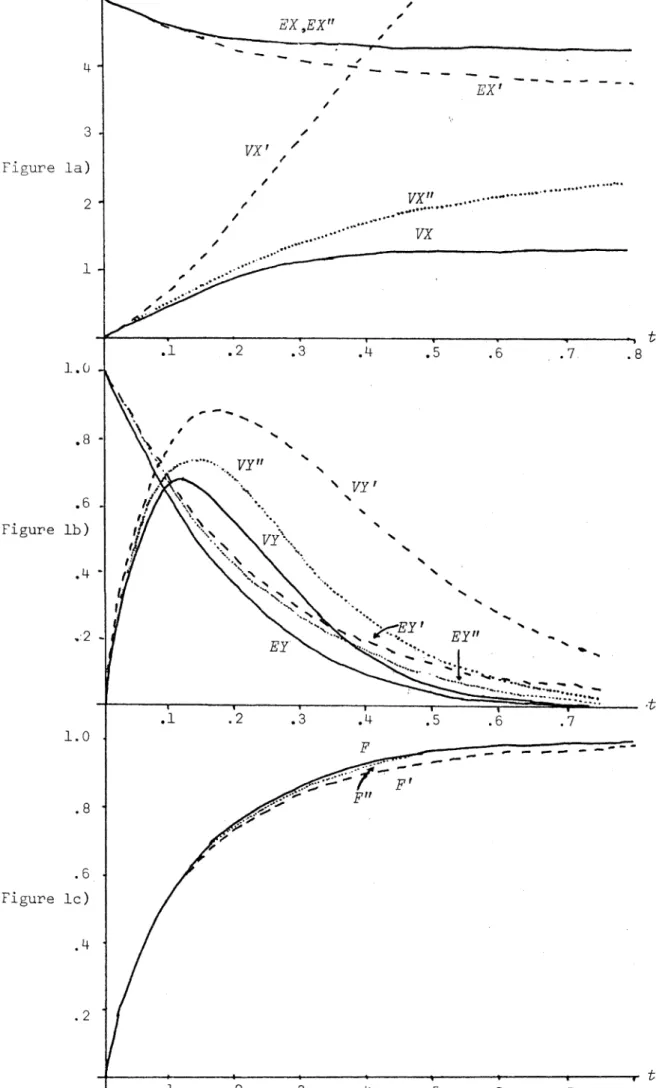
We evaluate the performance of the resulting approximating process with a series of graphs comparing real values (based on computer simulations) with their approximating values for various parameter values. As well as

this we find the joint p.g.f. for the process of Faddy by standard arguments since the method is more direct and the result in this form is more easily manipulated to give the quantities that we require, e.g. the distribution of

the duration time of the epidemic. The methods of Kendall (1956) are not applicable when the population is near critical (i.e. susceptible population size ~ relative removal rate). A suggestion is made for this situation which is supported by heuristic arguments and numerical results.

deterministic model, a simple formula is found for each generation size at any time, the formula resulting from a simplification of an expression by Daley (1967). The asymptotic form of the final generation size is found, thus generalising a result of Daley (1967) whose result is for the case when the relative removal rate is zero (the simple epidemic model). The rest of the chapter deals with the application of the approximating method of

chapter 3 and with the limiting result corresponding to that at the end of chapter 2.

In the general epidemic model it is implicitly assumed that the

population mixes homogeneously. It is this assumption which is most likely to be unsatisfactory in any particular application. It is natural therefore to consider a modification of the model which allows for the existence of subgroups within which mixing is homogeneous but between which it is more restricted. Such a model is the subject of chapter 5. Mathematical

difficulties are multiplied by the non-homogeneity, though some interesting results can still be obtained. The effect on the important threshold theorem

is examined both in the stochastic and deterministic cases. The probability of containing infection in the group in which it originates is found

approximately. The usual renewal arguments are applied yielding recursive expressions for mean final sizes of the epidemic in each subgroup and for the duration of the epidemic in the whole population. An analogous

approximating technique to that of chapter 3 is applied and the limiting diffusion process is given.

In chapter 6 we look at three models for epidemics in which the

The first of these is a model applicable to a population with little or no mobility. The model assumes that the disease is spread only by those

infectives on or adjacent to the boundary of the infected area. The

resulting process is a linear one and we are able to obtain expressions for the mean numbers of active infectives and also for the probability of

extinction of the process„

The second of the models of chapter 6 is a two-type branching process model applicable to a population with family structure. Branching processes are useful in describing the early behaviour of an epidemic process. This is particularly interesting because it is the behaviour of the epidemic during its early stages which will determine if the outbreak will be minor or majoro In the model we distinguish between infectives who were infected by members of their family and those infected by individuals not of their

family. A special case of this model is the model of Bartoszynski (1972). Our approach here is different, using branching process theory to obtain results about the moments of the two types of infective and the probability that the process will become extinct.

C H A P T E R 1

I N T R O D U C T I O N

1.0 I nt ro d u c t i o n

The general epidemic model is a mathematical model to describe the spread within a population of some characteristic able to be transmitted from one individual to another. We usually imagine the characteristic to be a disease although for some applications it may be a rumour or a particular item of information. The model assumes that the population consists of three types of individuals: susceptibles who may become infected by contact with infectives; infectives who have the disease and may cause further

infections by contact with susceptibles; and removed individuals who have, or have had, the disease and play no further part in the process because of immunity or isolation or death. Infectives become removed at a rate

proportional to the size of the infective population. Members of the population, except for removed individuals, are assumed to mix uniformly, and hence susceptibles become infected at a rate which is proportional to the sizes of the susceptible and infective populations.

The model was first introduced in a paper by Kermack and McKendrick (1927), No further work appears to have been done on the model until Bailey (1953) published a paper on the final size of the general epidemic. Shortly after, Whittle (1955) generalised the threshold theorem of Kermack and McKendrick to the stochastic case and Kendall (1956) introduced an

remaining uninfected by the process of the general epidemic model (hereafter simply called "the general epidemic") was investigated by Daniels (1965). Ridler-Rowe (1967) found the asymptotic form of the mean duration time of

the process. Asymptotic limiting processes were the subject of work by

Nagaev and Startsev (1970) and Barbour (1975). Abakuks (1973) investigated

the cost of the general epidemic and Watson (1972) studied a generalisation of the model in which the population is assumed to be stratified.

The rest of this chapter is a brief survey of known results about the general epidemic model which must be referred to in subsequent chapters.

1.1 The model

THE STOCHASTIC FORM

Let the number of susceptibles and infectives at time

t

be

X(t)

and

Y(t)

respectively (for convenience

t

will usually be suppressed). The

transitions from the state

(X, Y)

in the time interval (t,

t+6t)

are

given by

1.1

'U-i, y+i)

(x, y

)

+ ■

lu,

y

-

d

with probability

\iXY6t

+ o(6t) ,

with probability

yY&t

+ o(6t) ,

as

6t

-*• 0 .

The initial conditions are (Y(0), Y(0)1 = (n,

a)

. (The parameters y

and y are known as the contact rate and the removal rate respectively. It

is more convenient and more common to use the relative removal rate p = y/y

instead of the two parameters y and y . Thus it merely requires a change

in time scale to write the above infinitesmal transition rates as

XY

and

Let

p (£) = Prf(Z(t), 7(f)) = (r, s)} ,

V s

r = 0 , l 9 . . . , n , s = 0, 1, n+a-r .

Considering the possible transitions in the time interval (t, i+6t) and letting 6t ->• 0 leads to

1.2 p (t) = -s(r+p)p (t) + 0+ l ) ( s - l ) p At) + p(s+l)p (t) ,

rrs K r rs r r+l,s-l r r,s+l

r = 0, 1, . .., n , s = 0, 1, ..., n+a-r ,

where p (t) is defined to be zero if s is negative.

I1 s

X Y

Let P(w, z; t) - e[w z ) be the joint p.g.f. of (7, 7) . Multiplying 1.2 by rs and summing over the possible values of r and s shows that P satisfies the partial differential equation

1.3

dt = z{z-w)

f p _

dh)dz

v 9P + p(i-a) ^

where P(y, z\ 0) = jJ 1za .

Equations 1.2 and 1.3 are well known (see e.g. Bailey (1954)). Their solution has proved to be extremely difficult. Gani (1965) and Siskind (1965) obtained solutions using transform techniques. More recently Billard (1972) used matrix methods to find a solution in simpler form.

THE DETERMINISTIC FORM

From 1.3 it follows easily that

dEX

where Z is the number of removed at time t .

Assuming that we may write EXY - EXEY (which holds to a good

approximation in large populations), and writing x, y and z for EX, EY

and EZ respectively, we obtain the following equations which define the deterministic model corresponding to the stochastic model defined by 1.1:

1.4a) x - -xy ,

where (x(0), y(0), 3(0)) = (n, a, 0) .

It is easily seen that if n 5 p , y is always decreasing. This lies behind the important threshold theorem of Kermack and McKendrick which says that a major outbreak is only possible if n > p .

Combining 1.4a) and 1.4b) we have

1.4b) y = xy - py ,

1.4c) ^ = p y ,

1.5 - p i n — - z - n + a - x - y .

n a

Substituting for y from 1.5 into 1.4a) and integrating gives

1. 6 ds = ,

x s[n+a-s+pln(s/n))

From equations 1.4 it follows easily that y(°°) = 0 . Hence from 1.5

we see that 0 (= ^(°°)) , the number of susceptibles left after the epidemic

has become extinct, is the unique solution between 0 and n of the

equation

1.7 -p In —

n

0

- n \ a - 00

and we note that it is readily shown that

1.8 0 ~ n exp as n c° .

1.2 The distribution of the final size

The final size of the epidemic, W , is defined to be the number of

further infections (not counting the initial infections) that have occurred

at the time of extinction of the process. Let

.p (ft, a) - Prj(7 = r | (x(0), y(0)] = (n, a)] •

It is easily shown by a backwards equation argument that for v - 0 , 1 ,

1.9 p (n, a) - —7— p^ A n -1, a+1) + — *7— p (n, a-1) , n, a - 1, 2, ... ,

rr n+p r ^-l n+p rr

and

p (n, 0) = p (0 , a) - 6(r) ,

r r Y*

where

'l if a = 0 , 6(a) = 1

a n d w h e r e we d e f i n e p ^(n, a) = 0 , and p^(«, a) - 0 if r > n . E q u a t i o n

1.9 m a y be fo u n d in D aniels (1965) w h e r e it w as f u r t h e r e s t a b l i s h e d that

n-r r ^

1 -10

£ V r (n’

a )

=

A k n ~

fc=0 r+k) [p+r+k

n+a-r

n, a = 1, 2, . . . , ** = 0,1, . . . , « ,

w h e r e the A^ a re d e f i n e d r e c u r s i v e l y b y

n-r ( n-r

1 . 1 1 6 (n-r)Ak {T,k) _p+r+k) , « = 1, 2, . . . , ** = 0, 1,...,«..

D a n i e l s shows that the A* are f u n c t i o n s o f k, r and p only.

It w as sh o w n in B a i l e y (1954) that

m

1.12 V r=0

n - r

{n-mJ » > ■ o •

n = 1, 2, ... , m - 0, ..., n

U s i n g a h e u r i s t i c a r g u m e n t Daniels c o n j e c t u r e d that as n 00 ,

1.13 p («, a)

rn-r i-(£ )_n

a-fne~n / p )]

r\ cp(-ne -n/p>

It is w e l l - k n o w n that in the s u p e r c r i t i c a l case (n > p) W has a b i m o d a l d i s t r i b u t i o n . E p i d e m i c s o f int e r m e d i a t e size o c c u r w i t h v e r y low

p r o b a b i l i t y and the e p i d e m i c w i l l w ith h i g h p r o b a b i l i t y a f f e c t e i t h e r a very

s m a l l p r o p o r t i o n o f the s u s c e p t i b l e s in the p o p u l a t i o n or a v e r y large

p r oportion.

THE M E A N OF THE FINAL SIZE

n

C (n, a) = E[w I (7(0), 7(0)) = (n, a)) = £ a) •

p r=0 r

(We shall usually suppress p .) Multiplying 1.9 by r and summing over

v - 0, 1, . .., n yields

1.14 C(n. a) = [1+C(n-1, a+l)] + — - C(n9 a-1) , n, a = 1, 2, ... ,

9 n+p ’ n+p 9 5 5 9 9 9

and

C(n, 0) = 67(0, a) = 0 .

Substituting successively for the final term gives

a-1

1.15 C(n, a) = — —

Y,

-n Ls

n+9

k=0 n+p^

[1+C'(n-1, a+l-Zc)] ,

from which it is readily shown by induction that

1.16 _{C(n9 a)} = n - £ $ kak

k-1

n+a-k

where the

\

are defined recursively by

1.17

n

I

fc=i

O

k+p,

n-/c

= n n = 1

The results of this section may be found in Abakuks (1973) where 1.16

first appeared. It was later found as a special case in Lefevre (1978).

1 . 3 T h e d i s t r i b u t i o n o f t h e t i m e to e x t i n c t i o n

The epidemic is defined to be extinct when there are no more infectives

become extinct with probability one. Let

T

be the time to extinction and

Fy(t) its distribution function. Since

n

1-18

F (t) =

£ P r 0 U ) = F(l, 0;

t) ,

v

-0

and

P(x, y

;

t)

is known, in theory

t)

is known. In practice however,

the existing solutions for

P(x

,

y\ t)

mentioned in section 1.1 (and see section 2.1) are so complicated that this expression is completely useless

except for very small values of

n

and

a

. Barbour (197 5) has shown that

in the case where the initial conditions are (y(0), Y(0)) = (n,

nh)

, where

h

is constant, and the contact rate is

1/n

, then as

n

-*■ 00 ,

(p-<J>)T - In

n - k

converges in distribution to the random variable with distribution function

exp

[-e

, where <j) satisfies

1^+

h -

(J> + p In <J) = 0

and

k

= lim

m ^ °°

-In

m+(

p—(J))c7 1 +

m{

p-(p)J + In 1

-where

J(

a, B) r B

•'a

______

ds

______ s(1+^-s+plns)

The case when the initial number of infectives is constant is also

THE MEAN OF THE TIME TO EXTINCTION Let

M(n, a) = e{t | p( 0 ) , Y(0)) = (n , a)) .

The process may be looked upon as a random walk on the lattice (r, s) where r - 0, 1, n and s = 0, 1, n+a-r . From the state (r, s) the walk may go to (r-1, s+1) with probability r/(r+p) and to (r, s-1) with probability p/(r+p) . The time spent in (r, s) is an exponential variate with parameter s(r+p) . Hence it follows that

1.19 M(n, a) 1

a(n+p) n+p M(n-1, a+1) + — — M(nn+p , a-1)

n = 0, 1, . . a = 1, 2,

and

M(n, 0) = 0 .

This is a well known technique and equation 1.19 may be found in Billard (1977) .

By considering the process as a competition process and using theorems of Reuter (1957), (1961), Ridler-Rowe (1967) has shown that

1.20 M(n, a) r \ s _{— In(n+a)}

Y

as n -+ °° ,

where a is not necessarily a constant.

1.4 The stochastic threshold theorem

Let

where 0 5 f < 1 .

By considering birth and death processes that formed stochastic upper and lower bounds for the general epidemic process Whittle (1955) was able to show that for

n

large enough,

Hence if p >

n

, with probability 1 the process will become extinct before its size exceeds any given proportion of the initial susceptible population. This is the stochastic threshold theorem corresponding to the deterministic one of section 1.1.

Kendall (1956) introduced an approximating process by reasoning along similar lines as follows. In order to describe the early development of the process it is assumed that the effect of the depletion of the susceptible population during these early stages may be neglected. When

X

is held constant at its initial value

n

the process becomes a birth and death process

Y'

with birth rate

n

and death rate p (in fact

Y'

is a stochastic upper bound for

Y ).

If p >

n

extinction of

Y r

is

certain so few further infections are expected and hence

Y 1

is used as the approximation to

Y

. If p

< n

extinction of

Y r

occurs with probability

(p

/n)°

in which event it is known that

Y 1

behaves like a birth and death process with birth rate p and death rate

n

(see O'N. Waugh (1958)) so this process is used as'the approximation for

Y

. Also in the case p <

n

,

Y*

will not become extinct with probability 1 - (p

/n)a

in which event we use the deterministic variable

y

(see equations 1.4) as the approximation 1 o 21

for

Y

approximating system, C t(,ni a) , is given by

1.22

C'(n, a) = R-(£fl(n-e) + (sT

-BZ-_ KnJ J [nj n-p

1.5 A q u a s i - d e t e r m i n i s t i c a p p r o x i m a t i o n

Faddy (1978) considers an approximation to the general epidemic model as a special case in a more general discussion of a class of stochastic compartment models. In the infection probability rate the stochastic variable Y is replaced by its deterministic analogue y . The resulting process (X', Y') is mathematically tractable and it is shown that

1.23 Pr{(r, y p = p , s j )

n-r-s

1 r!s^!(rc-r-s^J !

and

1.24

where

Pn(t) =

x(t) n

p i2(t) =

k (y(t)-ae~pt)

>

and

The distribution of the number of susceptibles remaining uninfected after the extinction of the process is a binomial random variable with

mean 0 .

1.6 The a p p lic a tio n o f the general epidemic model to rumours

In the application of the general epidemic model to the spread of news or rumours the characteristic transmitted from one individual to another is thought of as being a particular rumour or item of knowledge. Thus an infective is an individual who knows the rumour and a removed individual is one who has heard the rumour and forgotten it. It is important in this application to consider not only if an individual is infected but to which generation of infection he belongs. (The

a

initial infections are regarded as belonging to the "Oth" generation of infectives, those infected by them to the 1st generation etc.) This is relevant because it would be expected that the distortion of the rumour increases as the generation "distance" from the source increases.

The model is essentially no different from the general epidemic model. The only change is that attention is now directed to the individual

generation sizes.

The following stochastic and deterministic models were first formulated by Daley (1967).

THE STOCHASTIC MODEL

Let

X

and

Y

, ^ = 0 , 1 , . . . , be the number of susceptibles and

d

g

th generation "knowers" respectively present in the population at time

Define

(X,

Y) 2

Y0,

r r . . . ) .

The inf initesimal transition probability rates are given by

U , Y) +

{

fX-1,

Yte

, ] at rate

\iXY

,

v 2+1' 9

fl, Y-e )

^ 9J

9 - 0, 1, . . .

at rate Y

Y

, 9

where e , £ = 0, 1, , is the vector with 1 in the (^+l)th place

and zero elsewhere» The initial condition is

(x(0), Y(0)) = (n, a, 0,0, ...) .

Define the final size of the

gt\\

generation,

W

,

g -

0, 1, ,

9

to be the number of

g

th generation removed at the time of extinction of

the process.

Let

a

= fa„, a,, ...,

a

.1

and define v O ’ 1* 5

m+lJ

(n, a) =

[ n

,

a^,

•

Further, let r = fr_, ...,

r

1 , e7 be the (fc+l)th row of the

v 0

m+lJ

k

(m+2) x

(m+

2) identity matrix and

Pjri

, a)

= Pr-jfv^ =

rgi g -

0,1, ..., m,

I, V

V i I

*(0)>

V 0)’

•••’

D y°>

K=m+1 ^ K=m+1

(n, a

)\ .

1.25 p (n, a)

(yn+y)

m

+1

I

k

=o

f

1 I Un[a^p (n-1,

r - e k + i

a+efcJ+YV >

+yna ,p (n-1, a+e _)+ya _p («, a-e .1 f , M m+rr-e 5 m+l' 'm + r r ' ’ m+r1 J

m+1 ;

Y l ~ 1 J 2, ... , CZq 5 (2^ 5 • • • •) ~ ^ 5 ^ * * * • 5

where any probability whose subscripts are either zero or whose sum exceeds

n

is defined to be zero, and

p r(0, a) = 6(r) ,

where

6(a)

'l if a = 0 ,

0 if a y 0 .

THE DETERMINISTIC MODEL

Let

x

and

yg

,

g

= 0, 1, ... , be the deterministic equivalents of

X

and

Y

and

z

,

g -

0 , 1 , ... , be the number of

g

th generation

w 3

removed at time

t

. The deterministic model corresponding to the stochastic model is defined by the equations:

1„26a)

x

=

-Vxy

,

1.26b)

•

y

= yxv . -

yy

,

_g

_{= o, 1, ••} • 5

1.26c)

•

z

= yy ,

0 T y 0 = 0» 1» •• * 5

where

y

= ]T

y

and

y

is defined to be zero, and where the initial <?=o ' 3

3 ( 0 ) = 0 , g - 0 , 1 , . . . .

Daley (1967) showed that

1.27

where

3

(t)

g

p

n

\n dv

g

_j

dv

g

J

_x(t)

_•

_u

ip(v)

exp

i

p(v)

u

1. 28 i

J

j

(

v

) = n

+ a -

V

+ p i n —

n

1.7 The general epidemic in a stratified population

This is an important extension of the general epidemic model which

attempts to make a more realistic assumption about the mixing of the

individuals in the population than that made by the general epidemic model.

The population is assumed to consist of m distinct groups in which

homogeneous mixing occurs but between which mixing is restricted. Thus in

the time interval (£, t+6t) an infected individual of the Jth group,

j = 1, . m , has probability y ..St + o(6t) , as 6t -* 0 , of infecting

O'^

any susceptible in the ith group, £ = 1, ...,

m

, where in general > ^ ’£ 5 f ^ J • The idea of considering the population as stratified

goes back to Rushton and Mautner (1955) and Haskey (1957). The following

formulation of both the deterministic and stochastic models is due to

Watson (1972).

THE STOCHASTIC MODEL

Let AT., AT ,

i

- 1, . .. , m , be the number of susceptibles and

infectives in the ith group at time t . Let X = (A^, ..., A^) ,

Y = (y , ..., Y } , y . be the ith column of the matrix {p..} and e.

be the ith row of the m x m. identity matrix.

The infinitesimaltransition probability rates for the model are given

by

(X-e^., Y+e^.)

at rate ,

1.29

(X, Y)

■( i =

1,

..., m ,

(X, Y-e^)

at rate ,

where as in section 1.6 we understand (X,

Y)

to mean

[X, , . .. , X , Y. , .. ., Y ) .

v 1 m l

m-The initial conditions are (X(0), Y(0)) =

(n, a)

, where

n =

[n. , . n

)

and

a =

fa,, ..., a ) .

v 1 K 1 mJ

Let

P(n

a ) (r, s,

t) = Pr{

(X

,

Y)

=

(r, s)

|

(X(o), Y(o)) =

(n, a)}

,

where

r

= fr, , ..., r ) and

S

= fs. , ... , s ) .

It follows from the forward equation that this function satisfies

1 ’30 p ( n , a ) ( r ’ s ’

t)

' .1

^ =l

y .a ,+n

.u . • a

z z z z

p (n,a)

(r, s, t)

* W

aP(n-ei ,a+ef ) ( r * S’ t)+W ( n , a - e , ) ( r ’ s ’ 4)_

0 » b , ... , 0 , 1 , ..., ,

= 0, 1, ..., n^+a^-r^ , £ = l, ..., m ,

where any

p (n,a)

(r, s ,

t) having subscripts for which some vz. > n

T = 1, ,.,, m , is defined to be zero, and

An equation equivalent to 1.30 was first stated by Billard (1976) where the stochastic model was presented in a form which would enable the application of her method of solution for the general stochastic epidemic model (see Billard (1973)).

THE DETERMINISTIC MODEL

Let ar., ,

i

= 1, ...,

m

, be the numbers of susceptibles ,

infectives and removed in the tth group at time

t

in the deterministic model. The model is described by the equations

1.31a)

m

x ^

-

-x^ £ s i ~ 1s • • •» m ,

1.31b)

m

y i = x i Z ~ y iyi ’ • • • > m >

0— 1

1.31c)

'

zi = y iyi ’

1

= X ’ *•* ’ m ‘

The initial conditions are (x^(0), y^.(0), 2^(0)] =

o) ,

i -

1, ...,

m .

Watson (1972) combines 1.31a) and 1.31c) to give

1.32

a:. m

ln s : = ^ vj i {nj +af xf yß ’ * = ••• ’ m •

As t h► °o , -> 0 , £ = 1, ..., m , so 1.32 becomes

1.33

0. m

in «7 = ^l ’

C H A P T E R 2

SOME T H E O R E T I C A L R ES U L T S ON THE G E N ER A L S T O C H A S T I C E P I D E M I C M O D E L

2 o0 I n t r o d u c t i o n

This chapter presents some theoretical results on the general

stochastic epidemic model formulated as a continuous time Markov chain on a finite state space. With the exception of the first section these results are asymptotic results valid as the size of the initial susceptible

population increases with other parameters remaining fixed.

In the first section we obtain a solution for the state probabilities at any time. The solution arises by writing the process in the form of a one dimensional finite Markov chain in continuous time and then using theorems from the general theory of linear differential equations. This method is simpler than existing methods for obtaining either the state

probabilities or the joint p.g.f. (see Gani (1965), Siskind (1965),

Billard (1973)) and the solution is in simpler form. Inspection of the form of the solution makes it difficult to imagine that it could be simplified further. Nevertheless it is still quite complicated.

of the process is taken into account.

Although simple recursive equations may also be found for the mean duration time of the epidemic, it was not possible to use the same technique to find the asymptotic form. We are able to use a heuristic argument which may also be applied to more complicated models. For this purpose we define here a modification of the general epidemic model which allows for an

arbitrary latent period between an individual's becoming infected and

becoming infectious. We find the asymptotic form of the mean duration time in this model and we also show that the distribution of the final size is the same as that for the usual general epidemic model.

The next section presents a process which is the limit of the general epidemic process under certain conditions. This process arose out of an attempt to put on a rigorous basis Kendall's idea of using a birth and death process to approximate the general epidemic process in its early

stages. Another limiting process which results when a different sequence of initial conditions is assumed is presented in the last section.

2.1

The s t a t e p r o b a b i l i t i e s

Any ordered pair (r,

s

) where

r

= 0, 1, ...,

n

and

s -

0, 1, ...,

n+a-r

, represents a possible state of the system with

r

denoting the number of susceptibles and

s

the number of infectives. The process is a two dimensional finite Markov chain on these states. By

enumerating the possible states uniquely we can regard the process as a one dimensional Markov chain.. Hence it may be described by the equation

2.1

pU)

=

Ap(t)

,

only one) p (£) and A is the matrix of infinitesimal transition

I O

probability rates. The theory of such a system is well known.

The following theorem gives the solution for the state probabilities in

our particular case under a mild restriction on the parameter p .

T H E O R E M 2 01.

If p is such that

j(£+p) p)

when (£, j) t- { i j') /or all integer pairs representing a possible state of the system, then the eigenvalues of A are distinct and

p (t) ^rs

n+a-i A ..t

l

I

i=1 J=1

r - 0, 1 s = 0, 1, ..., n+a-r ,

where

- -j(i+p) , i - 0, 1, ..., n , j = 0, 1, n+a-i ,

and the K fx. .1 are determined bu the recurrence relation

rs v ; ü

p(stl)*r,s+l M * t V s(r+p)]T S b i ^ + (r+1)(s-l)Xr+ljS- i h ^ ) = 0 ,

where (A_^ .) = 0 if r > n , s+r > n+a or s < 0 ard by tbe initial condition

p (0) f rs

1 1/ r = n j s - a 3 1

0 otherwise.

2 . 2 The mean f i n a l s i z e

The following theorem establishes the first term of an asymptotic series expansion for C(rc, a) .

THEOREM 2 02. For p a positive constant and a a positive integer.

n - C(n, a) = o(n a+2) , as n •*■<*> ,

P r o o f . We shall need a lemma, which shall be proved below, giving uniform convergence of the terms of the series in equation 1.16.

Another result is needed to prove the theorem, namely that the ,

defined in 1.17, are uniformly bounded. This follows from the result of Gani and Shanbhag (1974) that the are all positive and hence writing

1.17 in the form

k-1

=

1- I

J=1

k - l ]

J-1 J U + P j

k-j

we see that they are all less than or equal to one.

From lol6 we have

a-2

[n-C(n, a)] = n1 2 £ Q ka^

k= 1

n+a-k

- na-2

I ©

fc=l k+P, k+pj

n+a-k-1 ka^p

k+p

si 1

1—

1

Si

;

_

1

S

1

a-

2

< n p I +

I

k-

1

k=n-lVn]+

10

p

>+p.

n+a-k-1

where [a] means the greatest integer not greater than a

LEMMA 2 . 3 . For p a positive constant and a a positive integer3

(n) _P_

W

[fc+p^

n+a-k o [n i f k < n-Vn 3

o[n a ) i f n-Vn < k < n 3

as n 00 .

Proof.

By Stirling’s inequalities (see e.g. Feller Vol. I, p. 54) we have for k - 1 , . . . , n- 1 ,

2.2 n % )

n+a-k

V(2rr) *+P

n+a-k n+%

n SXP

1 1 1

12« 12&+1 12(n-fc)+l

VtT

Ä7rf pn

k+pj

pn ©

k / { n - k ) pn

k+p

k ( n - k )

ci( \ n - k

n - k

/ pen

\fc~(n-k)

Consider now the 4 cases (i) fc < 3pe ,

(ii) 3pe < k 5 n-Vn ,

(iii) n-Vn < k < n -2pe , (iv) n - 2 p e < k < n .

The lemma is trivial for cases (i) and (iv). For case (ii) we have from 2.2, taking Vn > 3pe ,

VwnaQ

n+a-k

} < + p j

pn k+pj

a t

pen n - k

/ a ( v W n < n (%)

|3pe(n-3pe)

n > 9pe .

r \n+a-k a r N

p < p n 1 pen [

U + p J n-Vn+p \2pe{n-2pe)J

a 2pe

P (%) + 1 n > N , some /V

We note that in the Kendall approximating process discussed in

section 1.4 the mean final size is given by 1.22. From 1.8 we would expect that as n -*■ 00 ,

n - C(n, 1) = p + o(i) .

This was also conjectured in Abakuks (1973). The next theorem extends the asymptotic expansion of C(n, a) and establishes the truth of this

conj ecture.

THEOREM 2.4.

Under the conditions of Theorem 2.2,

C(n, a) = n - p

P

n

a-1

+ o [n , as n -* «>

Proof.

From Theorem 2.2 we may write

2.3 C(n, a) = n - ot (a) ,

n

where

a (a) = o(n a + 2] , as n 00 .

Now

C(n, 1) = [1+C(n-1, 2)] n from 1.14.

Substituting from 2.3 gives

Therefore

2.4 a (1) =

P

+ ° ( D , as ft -*■ 00 .

Substituting 2.3 in 1.14 for a > 1 gives

n - a (a)

n

=

0

!- < v

1

(a+i>]

[n+pj + [ft-a (a-l)lL n J

_l^+Pj

Therefore

a (a ) = a (a-1)

n n

P n^ + o

( -a+l'v

l” ' J

\a-1

P r -a+l\

\n) + ° ln J , as n -> 00 ,

from 2.4.

In principle it is possible by the method of establishing Theorem 2.4

to find the expansion of C(n, a) up to terms of any order. However the

algebra quickly becomes tedious and we assert without proof the further

refinement

2.5 C(n, a) - n - p

f

[

f

p

t

r

j

a(a+1) 2

■\CL +1 P

a

P

[(a+3)(a+3p)+2]

a\ 2

as n 00 .

The expected final size was calculated using equation 1.14 for various

values of the parameters p, a, n . The following tables compare the true

values of n - C(n, a) with the approximations calculated from equation 2.5

(shown in brackets). The approximation seems fairly insensitive to

variation in the parameter a . As we would expect it is useless for

p/n ~ 1 but surprisingly good for values of p/ft as large as .5 , even

P = 1

a

1 2 3

5 1.12 (1.84) 0.29 (0.31) 0.09 (0.09)

10 1.03 (1.03) 0.11 (0.11) 0.01 (0.01)

25 0.00 ( 1.00) 0.04 (0.04) 0.00 (0.00)

P = 2

1 2 3

5 2.15 (3.12) 1.03 ( 2.07) 0.53 (1.33)

10 2.22 (2.16) 0.57 (0.49) 0.19 (0.12)

25 2.01 (2.01) 0.16 (0.16) 0.01 (0.01)

P = 5

1 2 3

5 3.69 ( 19.2) 2.77 ( 42.8) 2.12 (77)

10 5067 ( 6.9) 3.48 (5.05) 2.31 (3.69)

25 5.31 (5.15) 1.28 ( 1.08) 0.42 (0.23)

We note that the approximation for C(n, a) given by 1.22 may be written

C'(n, a) = n - p

P

k

a-1

+

a

P

,n ,

a+1

+ o [n a , as n

which agrees with 2.5 as far as the term in n-a-1

2.3 The s e c o n d m o m e n t o f the final size

O ' fr

D( n, a) = t f ( j r I ( j ( 0 ) , Y( 0 ) ) = ( n , a ) ] = £ r p ( n , a ) . r =0

M u l t i p l y i n g e q u a t i o n 1 . 9 by r a nd summing o v e r r - 0 , 1 , . . . , ft , we o b t a i n

2n u o

2 . 6 Z?(n, a ) = — C { n -1 , a + l ) + — [ 1 + D ( n - 1 , a+1 ) ] + D{ n, a - 1 ) ,

n , a = 1 , 2 ,

S u b s t i t u t i n g s u c c e s s i v e l y f o r t h e f i n a l t e r m g i v e s

a - 1 r \ k

2 . 7 D ( n , a ) = X 7T~x D ( n -1 , a + l - f c ) + 2C(m, a ) - 1 +

n + P fc=0 l«+PJ

From 2 . 7 we may r e a d i l y p r o v e by i n d u c t i o n t h a t

2 . 8 Z?(n, a ) = 2n C( n , a ) - r ? + £ Zc=l

P n+ a-k

w h e r e t h e b-, a r e d e f i n e d by

2 . 9

n l

k- 1 fc+p.

w-Zc

2

n , n 1 , 2

We now n e ed t h e f o l l o w i n g lemma wh i c h g i v e s t h e o r d e r o f m a g n i t u d e o f

t h e b , .

k

LEMMA 2 . 5 . For n = 1 , 2, . . . ,,

n < b 5 n 2 . ( l + p j w

Proof. From 2 . 9 we h a v e = 1 a nd b^ = 2 ( 2 + p ) / ( l + p ) s o t h a t t h e

l o w e r b ou nd h o l d s f o r n - 1 , 2 . Assume t h a t t h e l o w e r b ou n d h o l d s f o r

2.10 b - m‘

m

1 '"»‘«tel

m-k - m m-1

I

k=1 m-1 k

r \m-l-k

P fe+pj

mp

(m-k)(k+p)

Now (m-k)(fc+p) for k - 1, m-1 , has its minimum at (w-l)(l+p) . By the induction hypothesis all the ..., b^ ^ are positive, therefore

b > m 2 -

m l+p

m(m+p) l+p

Hence by induction b^ > n(n+p)/(l+p) for all positive integers n . It

2

now follows trivially from 2.10 that b^ < n for all integers n 4 □

COROLLARY.

Under the conditions of Theorem

2.2^

2.11 (i) I Q b

k=1 * fc + P, n+a-k

= c>f -a+3^[n J as n 00 j

2 „12 (YiJ Z?(w, a) - n - p‘ P a-2

+ p (a-1)

i»J +

p)a 1 r -a+l>

)

as n 00

2.13 fiiij F(n, a) = p‘ P nj

a-2

+ p (a-1)

r ,»a:-l

* °(

m

) .

as n -*■ 00 j

where V{n, a) = Var(V | (l(0), 7(0)) = (w, a))

Proof.

The proof of (i) is exactly the same as that of Theorem 2.2,

ft2 - D(n, a) - o[n a+3) , as n -* 00 ,

and then extending the expansion using the same method as in Theorem 2.4.

(iii) is a trivial extension of (ii).

2 A T h e m o m e n t s c o n d i t i o n a l on a m a j o r o u t b r e a k

As stated in section 1.2 an important feature of the distribution of

the final size is that it is bimodal. The first mode of behaviour

corresponds to early extinction of the process in which only a small

proportion of susceptibles are infected and the second to a major outbreak

affecting a large proportion of the susceptible population. The discussion

in section 1.4 shows that in the case n >p , we can approximate the

probability of early extinction by (p/n)a (see also section 2.6) and the

process conditional on this eventuality by a birth and death process having

birth rate y and death rate pn . Hence, if we let W be the final size,

W' the final size conditional on early extinction and W" the final size

conditional on a major outbreak we have

2.14 hO-#(W )Pr{early extinction}

1-Pr{early extinction}

E( W)

-\a - r

P a p

■

1

->

P

[nj n-p_ _{l n J j}

= n a(a+3)

2

( ^a+l

P

n.j

2a-1

using 2.5.

Hence we see that the term p(p/n)a ^ appearing in 2.5 is the result

of the probability mass of the first mode of the bimodal distribution of

2.15 VariW") - p ( a - 1 )

a-1

+ p P 1n>

2a-2

Comparing this with 2.13 we again conclude that the dominant term of the variance arises from the bimodal nature of the distribution.

2.5 The distribution of the final size

We may readily apply the methods of the previous section to other recurrence relations. Substituting successively for the final term in equation 1.9 leads to

2.16 p^(n, a ) n n+p a-1

I

k=0 ( \ P *+P. k

p A n -1, a+l-k)

r r - 1

a

Si r)

which gives

p Q(n, a)

|n+pj

P-^in, a) - n

Yl-l + P

a+1

n-l+p tn+pj

and so on. Rearranging this latter equation we have

n-l+p

l

P

J

p_(n,

0

a) +

. 'i a + 1

n-l+p . .

— -— p 1(n, a) = a ,

which is equation 1.12 for m = 1 , and in fact 1.12 follows easily from 2.16 by induction on v .

We now consider equation 1.10. The quantity p^(n, a) is of interest

and it is conjectured that pyin, a) -* 1 as n -> 00 . To justify this

1 . 1 0 and 1 . 1 1 become

Pn (n, a ) = 1 - I

rC ~ -L

f \

p+k

n+a-k

5 ^ 1» 2, . . . , (2 0 , 1 , . . . ,

w h e r e t h e c . a r e d e f i n e d r e c u r s i v e l y f o r k = 1, 2, . . . , by

2 . 1 7

1L

X 0

fc=l

IP+^J

= 1 , w = 1 , 2 ,

Now i f i t c a n be shown t h a t t h e o^ a r e u n i f o r m l y b o u n d e d t h e n Lemma 2 . 3

g u a r a n t e e s t h a t t h e sum a p p e a r i n g i n 2 .1 7 i s o[n a+^>j as n -y oo # i n t h e

c a s e p - 1 we may show by i n d u c t i o n ( p r o c e e d i n g a s i n Lemma 2 . 5 ) t h a t a l l

t h e a r e b e t w e e n 0 a n d 1 . F o r p > 1 a h e u r i s t i c a r g u m e n t a n d

c o m p u t e r c a l c u l a t i o n s s u g g e s t t h a t t h i s i s a l s o t r u e .

The r e s u l t i s r e a d i l y e s t a b l i s h e d h o w e v e r b y a r g u i n g a s f o l l o w s . (We

a r e i n d e b t e d t o D r. M. Faddy f o r s u g g e s t i n g t h i s a p p r o a c h . )

E q u a t i o n 4 . 3 o f D a n i e l s ( 1 9 6 7 ) s t a t e s t h a t

n+a-k

Pn_k ( n, a , p ) = $ ( p+fe) pn ( n - k , a , e + k ) ,

w h e re t h e e x t r a p a r a m e t e r p f o r t h e r e l a t i v e r e m o v a l r a t e o f t h e p r o c e s s

h a s b e e n i n t r o d u c e d i n t o t h e f u n c t i o n p (n, a ) .

p ( n , a , p ) = 1 - I p A n , a ,p) k- 1

= 1 - 1 0

k-1 ,P+k

n+a-k

p ^ ( n - k 9a, p+k)

Now s i n c e t h e p ^ ( n - k , a ,p+/c) a r e u n i f o r m l y b o u n d e d t h e r e s u l t f o l l o w s

Hence we may u s e t h e r e c u r r e n c e r e l a t i o n 1 . 9 a n d t h e m eth od o f

2.18 Pn(n, a) = 1 - + o(w a) , as

2.6 The p r o b a b i l i t y o f e a r l y e x t i n c t i o n

It has long been accepted, following the arguments of Kendall (see section 1.4), that the probability of early extinction in a general epidemic

its opposite "major outbreak" has- yet to be defined. The above-mentioned result is obtained by arguing that early extinction occurs if the birth and death process with birth rate n and death rate p becomes extinct. This criterion is chosen because such a process approximates the general epidemic process in it's early stages, since in the early stages we may ignore the effect on the contact rate of the small depletion in the number of

susceptibles. It would be more appropriate that the final size be the sole criterion for deciding whether a major outbreak has occurred. Here we discuss the probability of early extinction under such criteria.

with p < n is (p/n)a . Exactly what is meant by "early extinction" or

Let

qr(n, a) = Pr{^ < r | (*(0), 7(0)) = (n, a)} .

By the usual argument

2.19 q (ft, a)

-n, a = 1 , 2 , . . . , r = 1, ,. ., n ,

These probabilities may easily be calculated from these equations.

Referring to equation 1.21 we see that as long as r = o(n) as

n •+ 00 ,

q (n, a) ~ — , as n ■+ 00 . nj

It seems very difficult to obtain this result under more general conditions

on r . Equation 2.18 suggests that it is true even for r = n .

As in Theorem 2.4 we may use the recurrence relation 2.19 to find

further terms in the series for q^{n^ a) . Thus we may show that

2.20 qr(n, a) =

[4

a(a+3)

2p

(£)

[nj

a+2

( - a - 2 \

+ o[n

J ,

as n

2.7 The m e a n d u r a t i o n tim e

Equation 1.19 is of the same form as equations 1.9 and 1.14.

Proceeding in the same manner we find that

1 1

2.21 M(n, a) = — — Y — j- + nM(n-l9 a+l-k)

n+P

J

It was expected that expressions of the form of 1.10 and 1.16 could be

obtained from 2.21 and the asymptotic result of Ridler-Rowe (1967) that

M(n, a) — I n(n+a)

Y

as n 00 ,

could be obtained using the algebraic methods of sections 2.2 and 2.3.

Unfortunately this has not been possible, but the following heuristic

argument may be applied.