The Response of the Ozone Layer to Quadrupled CO₂ Concentrations

The Response of the Ozone Layer to Quadrupled CO

Concentrations

G. CHIODO,aL. M. POLVANI,aD. R. MARSH,bA. STENKE,cW. BALL,d,c E. ROZANOV,d,cS. MUTHERS,eANDK. TSIGARIDISf,g

a_{Department of Applied Physics and Applied Mathematics, Columbia University, New York, New York} b_{National Center for Atmospheric Research, Boulder, Colorado}

c_{IAC ETH, Zurich, Switzerland}

d_{Physikalisch-Meteorologisches Observatorium Davos, World Radiation Center, Davos, Switzerland} e_{Deutscher Wetterdienst, Research Center Human Biometeorology, Freiburg, Germany}

f_{Center for Climate Systems Research, Columbia University, New York, New York} g_{NASA Goddard Institute for Space Studies, New York, New York}

(Manuscript received 23 July 2017, in final form 7 February 2018)

ABSTRACT

An accurate quantification of the stratospheric ozone feedback in climate change simulations requires knowledge of the ozone response to increased greenhouse gases. Here, an analysis is presented of the ozone layer response to an abrupt quadrupling of CO2concentrations in four chemistry–climate models. The

au-thors show that increased CO2levels lead to a decrease in ozone concentrations in the tropical lower

stratosphere, and an increase over the high latitudes and throughout the upper stratosphere. This pattern is robust across all models examined here, although important intermodel differences in the magnitude of the response are found. As a result of the cancellation between the upper- and lower-stratospheric ozone, the total column ozone response in the tropics is small, and appears to be model dependent. A substantial portion of the spread in the tropical column ozone is tied to intermodel spread in upwelling. The high-latitude ozone response is strongly seasonally dependent, and shows increases peaking in late winter and spring of each hemisphere, with prominent longitudinal asymmetries. The range of ozone responses to CO2reported in this

paper has the potential to induce significant radiative and dynamical effects on the simulated climate. Hence, these results highlight the need of using an ozone dataset consistent with CO2forcing in models involved in

climate sensitivity studies.

1. Introduction

An accurate quantification of the effects of anthro-pogenic emissions on the ozone layer is a key step toward making accurate predictions of the future ozone evolution. Assessing the ozone response to anthropo-genic forcings is also a step toward improved un-derstanding of the coupling between atmospheric composition and climate (Isaksen et al. 2009).

There is robust modeling evidence suggesting that anthropogenic greenhouse gases (GHGs), via their in-fluences on stratospheric temperature and the Brewer– Dobson circulation (BDC), will greatly modify the

future distribution of ozone in the stratosphere (WMO 2014, chapter 2.4.2). More specifically, GHGs induce stratospheric cooling, but also strengthen the BDC. The cooling and BDC strengthening have opposite in-fluences on the ozone layer in the tropics: radiative cooling slows down ozone catalytic cycles and affects gas-phase ozone photochemistry (thus increasing ozone concentrations), while the strengthening of the BDC enhances advection of ozone-poor air in the tropical lower stratosphere, thus decreasing ozone concentra-tions (Shepherd 2008). However, the exact contribution of single forcing agents is unclear.

Among all well-mixed GHGs, CO2 is the dominant anthropogenic forcing agent on the climate system (Myhre et al. 2013), and is the key to the very definition of climate sensitivity (Andrews et al. 2012;Forster et al. 2013). Since increasing CO2 causes large radiative cooling in the stratosphere (Shine et al. 2003), and since ozone chemistry is temperature dependent, ozone concentrations change

Supplemental information related to this paper is available at the Journals Online website: https://doi.org/10.1175/JCLI-D-17-0492.s1.

Corresponding author: G. Chiodo, [email protected]

DOI: 10.1175/JCLI-D-17-0492.1

considerably upon abrupt CO2 increases. Furthermore, ozone is not a well-mixed gas, and responds to the circu-lation changes caused by increased CO2 concentrations (Garcia and Randel 2008). The ozone response to in-creased CO2levels, therefore, has the potential to be an important chemistry–climate feedback affecting both cli-mate sensitivity (Nowack et al. 2015) and dynamical sen-sitivity (Chiodo and Polvani 2017). Similarly, interactive ozone chemistry can play an important role in modulating the modeled response of ENSO to global warming (Nowack et al. 2017). Moreover, interactive ozone also dampens the climate system response to solar forcing (Chiodo and Polvani 2016;Muthers et al. 2016), and re-duces biases in paleoclimate simulations (Noda et al. 2017). It thus follows that an accurate quantification of the ozone response to external forcings is needed.

Intermodel comparisons of chemistry–climate models (CCMs) have provided useful insights into scenario-and model-related uncertainties in ozone projections (Eyring et al. 2010, 2013; Iglesias-Suarez et al. 2016; Butler et al. 2016). These studies inferred the effects of increased GHG levels on ozone by analyzing the sensi-tivity of ozone projections to different GHG emission scenarios. However, this approach does not isolate the impact of CO2alone, since CH4and N2O vary among each of the scenarios, potentially offsetting the effects of CO2 (Revell et al. 2012) because of their chemical re-activity in the stratosphere. Moreover, the comparison of different scenarios may be misleading because of nonlinearities from the combined effects of ozone-depleting substances (ODSs) and GHGs (Meul et al. 2015;Banerjee et al. 2016). Other studies were able to isolate the effects of GHGs (Zubov et al. 2013;Meul et al. 2014;Langematz et al. 2014), but did not quantify the impact of CO2alone.

Further motivation for an analysis of the ozone re-sponse to CO2 comes from the existing spread in the magnitude of the ozone feedbacks on equilibrium cli-mate sensitivity (ECS), where CO2is the only forcing (Nowack et al. 2015; Dietmüller et al. 2014;Muthers et al. 2014;Marsh et al. 2016). It has recently been shown that stratospheric ozone, in response to CO2increases, can reduce the estimated ECS by up to 20%, quantified as the temperature response to an abrupt quadrupling of CO2 (Nowack et al. 2015). However, other models show a smaller effect, ranging from 7%–8% (Dietmüller et al. 2014;Muthers et al. 2014) to nothing at all (Marsh et al. 2016). It is necessary to narrow down the un-certainty in the effect of ozone on ECS by understanding the sources of the existing spread. One of the possible sources of uncertainty is the ozone response to CO2. In Marsh et al. (2016), it was pointed out that there was qualitative agreement in the pattern of the modeled

ozone response despite the large variance in the size of the chemistry feedback. However, a detailed intercomparison of the modeled ozone response to increased CO2concentrations is still lacking: this is the goal of the present paper.

We examine the ozone response to an abrupt qua-drupling of CO2 in four different CCMs. Using four different models allows us to identify the robust fea-tures, and to quantify the intermodel spread. CO2is the only external forcing in these runs: this facilitates the attribution of the forced response. Moreover, the large instantaneous forcing from a quadrupling of CO2 con-centrations allows us to distinguish fast and slow re-sponses (Gregory and Webb 2008;Taylor et al. 2012), thus providing insights into the mechanisms driving the ozone response. Last, the longitudinal structure of the ozone response is analyzed in detail to highlight asym-metries in the ozone response, a feature that is presently omitted in ozone forcing datasets (Cionni et al. 2011).

The present paper documents the ozone responses to CO2 obtained in the different CCMs. The ozone responses in the four models will then be used in a follow-up study to quantify the feedback in the form of radiative forcing, and dynamical effects of ozone and its zonal asymmetries on the atmospheric circulation.

2. Models and method

a. Models

as p3 (physics-version53) in the CMIP5 archive. More details about the model physics and dynamics are given inSchmidt et al. (2014).

The GFDL CM3 model has a resolution of 2.58 lon-gitude by 28latitude and 48 vertical layers, with a model top at 0.017 hPa (;60 km). The ocean model component of CM3 is the Modular Ocean Model (MOMp1;Griffies et al. 2005). As in GISS-E2-H, this model includes clouds–aerosol interactions. The atmospheric compo-nent includes modules for tropospheric and strato-spheric chemistry, based onHorowitz et al. (2003)and Austin and Wilson (2006), respectively. Tropospheric and stratospheric chemistry modules have been merged, which implies extending the tropospheric chemistry module to include 63 chemical species, halogens, atomic hydrogen, and oxygenated species, as well as PAN and other ozone precursors. Details of the GFDL CM3 model physics can be found inDonner et al. (2011).

The CESM(WACCM) model has a resolution of 1.98 longitude by 28latitude and 66 vertical layers, with a model top at 5.96 3 1026hPa (;140 km). The ocean component is provided by the Parallel Ocean Program, version 2 (POP2). CESM(WACCM) is fully docu-mented inMarsh et al. (2013). The model includes a fully interactive stratospheric chemistry module, based on version 3 of the Model for Ozone and Related Chemical Tracers (MOZART; Kinnison et al. 2007), which in-volves 217 gas-phase reactions, and the advection of a total of 59 species. This version of CESM(WACCM) also includes a simplified representation of tropospheric chemistry, which is limited to methane and CO oxida-tion [seeMarsh et al. (2013)for more details]. We note that CESM(WACCM) does not include aerosol indirect effects.

The SOCOL model has a spectral resolution of T42, corresponding to 2.88longitude by 2.88latitude, 39 ver-tical levels, and a top at 0.01 hPa (;80 km). Ocean coupling is provided by the ocean–sea ice model Max Planck Institute Ocean Model. An accurate description of the model physics and chemistry is given inStenke et al. (2013). Atmospheric chemistry is calculated through 140 gas-phase reactions, 16 heterogeneous re-actions, and advection of 41 chemical species. The transport of the chemical species, including ozone, is calculated by the advection scheme of the middle-atmosphere ECHAM5.

All four models have model tops well above 1 hPa (;50 km) and have a well-resolved stratosphere. Therefore, they are considered ‘‘high top’’ models (Charlton-Perez et al. 2013). Most importantly, they include fully interactive stratospheric ozone chemistry: thus, the interplay between ozone chemistry, radiation, and dynamics is fully represented in all of them. There

are some differences in tropospheric ozone chemistry, due to the representation of feedbacks between climate and lightning NOx. In GISS-E2-H, GFDL CM3, and CESM(WACCM), lightning NOx sources are in-teractive and thus respond to changes in climate, while in SOCOL, they are prescribed through a climatological source of 4 Tg (N)/yr21. The complexity of the tropo-spheric chemistry mechanism differs among models, with some (e.g., GFDL CM3) including more reac-tions and species than others [SOCOL and CESM (WACCM)]. However, ozone responses in the tro-posphere are dwarfed by those in the stratosphere, as shown below.

b. Model experiments

We analyze two different forcing scenarios from each of the CCMs: a preindustrial (PI) control and an abrupt 43CO2scenario of equal length (150 yrs long), in which atmospheric CO2is instantaneously quadrupled at the beginning of the run. It is important to stress that ODSs and tropospheric ozone precursor emissions are held fixed to PI levels in both integrations: this is a key dis-tinction between 43CO2forcing and the emission sce-narios analyzed in earlier studies (e.g.,Oman et al. 2010; Eyring et al. 2010,2013;Iglesias-Suarez et al. 2016).

For CESM(WACCM), we use the same data analyzed in Marsh et al. (2016) andChiodo and Polvani (2017). For SOCOL, we analyze the output documented in Muthers et al. (2014). Where it is shown, we assess the equilibrium response of ozone to CO2by taking differences between the climatology obtained from the last 50 years of the 43CO2 integrations and the climatologies obtained from the 150 yr-long PI control integrations. After 100 years, ozone trends are found to be very small. Thus, these climatological dif-ferences will be referred to as ‘‘equilibrium response,’’ al-though they do not strictly represent a new steady state.

3. Results

a. Annual-mean ozone response

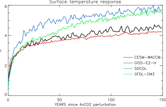
The time evolution of the global mean surface tem-perature response to 43CO2in the four models is shown inFig. 1. All models exhibit rapid surface temperature increase over the first 10–20 years following the CO2 quadrupling, and then warm at a smaller and more model-dependent rate. Over the simulated period, the warming ranges between 4.2 K (GISS-E2-H) and 5.8 K (SOCOL). Over the first 150 years, the warming in CMIP5 models in CO2quadrupling experiments typically ranges between 3.0 K and 6.2 K [see Table S1 inGrise and Polvani (2014)]. The key point here is that the four CCMs span over a good fraction (;50%) of the existing spread in climate sensitivity (measured as surface temperature response to 43CO2) across the CMIP5 models.

The equilibrium response in zonal-mean ozone, cal-culated as relative change, along with the tropopause

diagnosed using the WMO definition (WMO 1992),1is plotted inFig. 2. In the stratosphere, we identify a robust pattern of ozone response in the low latitudes, which consists of an increase by up to 30%–40% in the upper stratosphere (1–10 hPa), and a decrease of similar magnitude in ozone in the tropical lower stratosphere (TLS) (30–100 hPa). Relative changes near the tropo-pause are large (30%–50%). However, in (absolute) mixing ratio terms, the decreases in the lower strato-sphere are smaller than the increases in the upper stratosphere (see Fig. S1). Despite their small size in terms of volume mixing ratio, ozone changes in the lower stratosphere are particularly important for the global energy budget (Lacis et al. 1990).

The upper-stratospheric ozone increase has been un-derstood to be a consequence of changes in odd oxygen loss cycles because of CO2-induced cooling (Haigh and Pyle 1982;Jonsson et al. 2004). In this region, all models show a similar cooling of up to 16 K (Fig. 3). Assuming photochemical equilibrium, and following the analytical calculation presented in Jonsson et al. [2004; their Eq. (7)], a216 K temperature change at 1–5 hPa would lead to an 11% increase in the reaction rate coefficient involved in recombination (O1O21M/O3), and a 44% decrease in the reaction rate coefficient involved in ozone destruction (O3 1 O / 2O2). Combining the

FIG. 1. Global mean temperature response to 43CO2in the four CCMs, shown as departure

from the climatology of the respective control simulation (units: K).

1_{It is defined as the lowest level at which the lapse rate decreases}

effect of both reaction rate coefficients, and assuming no changes in OH, NO2, and ClO concentrations, we cal-culate an ozone increase of ;27% at 5 hPa, which is close to the values calculated by the models and explains the robustness of the upper-stratospheric ozone signal in the different CCMs.

In the lower stratosphere, the decrease in ozone concentrations is likely due to an acceleration of the BDC (Butchart 2014); both stratspheric cooling and the BDC strengthening are robust features in climate change simulations, and also dominate the ozone re-sponse to 43CO2.

In the troposphere, a dipole of ozone increases in the midtroposphere and decreases close to the tropopause layer is seen in all models. The pattern of tropospheric ozone response to CO2has been linked to enhanced NOx lightning, and uplifting of the tropopause (i.e., ozone-poor tropospheric air replacing stratospheric air; Dietmüller et al. 2014). In the middle troposphere, enhanced NOx lightning can result from changes in both the intensity (depth) of individual convective events, and the overall frequency of convection with warming (Banerjee et al. 2014). Enhanced NOx in the free troposphere can lead to more efficient ozone production via cycling of HOx and NOx radicals (Brasseur and Solomon 2005).

The SOCOL model is consistent with the other models in projecting an ozone increase in the tropical and subtropical upper troposphere (300 hPa), despite the lacking response in lightning NOx emissions to CO2 increase in this model. This suggests that tropospheric

FIG. 2. Relative annual-mean zonal-mean ozone response in (a) CESM(WACCM), (b) GFDL CM3, (c) GISS-E2-H, and (d) SOCOL (units: %). The thick violet solid (stippled) line identifies the tropopause in each of the models for the control (43CO2) experiment, calculated

using the WMO lapse rate definition. Regions that are not stippled are statistically significant (at the 99% level), according to thettest.

ozone increases can be driven by other processes, such as stratosphere–trosphere exchange (STE;Hegglin and Shepherd 2009;Garny et al. 2011). The specific pattern, with a positive ozone response extending from the sub-tropical upper troposphere poleward and upward to the lower stratosphere in the midlatitudes, is a further in-dication that STE could contribute to the tropospheric ozone response to CO2.

There are also some notable intermodel differences in the magnitude of the stratospheric ozone response in the tropics. In the upper stratosphere, the ozone increase ranges from 40% in CESM(WACCM) and GISS-E2-H, to 30% in SOCOL and GFDL CM3. In the TLS, the decrease in ozone concentrations ranges from 50% in SOCOL to 30% in CESM(WACCM). These intermodel differences are more evident when looking at ozone volume mixing ratio (Fig. S1). Some differences among models are also present in their PI control climatology (Fig. S2), although these are generally smaller than the response to CO2, especially at low latitudes.

To bring out the intermodel differences in the tropical ozone response to CO2, we show the annual-mean tropical average (308S–308N) profile of ozone mixing ratios inFig. 4. First, we note differences in the location of the peak in the upper-stratosphere (3–5 hPa) ozone increase, with GISS-E2-H and CESM(WACCM) showing a peak at higher altitudes than SOCOL. Sec-ond, while models agree in the location of the maximum ozone decrease at 30 hPa, there is significant intermodel

spread in amplitude; the ozone decrease ranges between 0.2 ppmv [GISS-E2-H and CESM(WACCM)] and 1.0 ppmv (SOCOL). Third, one can easily see that tro-pospheric ozone changes are extremely small compared to those occurring in the stratosphere. In the following section, we will show that the spread in tropical lower-stratospheric ozone is consistent with intermodel dif-ferences in the BDC, and tropospheric temperature.

There is some coherence between intermodel spread in tropical stratospheric ozone and temperature. For example, SOCOL shows the largest ozone decrease at 30 hPa, and is also the model with the largest cooling in response to CO2, between 50 and 10 hPa (Fig. 3). The opposite is seen in CESM(WACCM): a weaker TLS ozone decrease in this model could explain the weaker cooling at 30–10 hPa. This suggests that ozone responses may contribute to intermodel spread in the stratospheric cooling because of increased CO2levels. Nevertheless, there is no relationship between temperature and ozone response in GISS-E2-H, suggesting that other processes, perhaps dynamical cooling or stratospheric water vapor (e.g., due to intermodel differences in the strength of the stratospheric water vapor feedback; see Dessler et al. 2013), may also contribute to the intermodel spread in the stratospheric temperature response to CO2.

b. Column ozone response

Next, we vertically integrate the response displayed in Fig. 2 to quantify the equilibrium response in total

FIG. 4. Tropical mean (308S–308N) annual-mean, zonal-mean ozone response to 43CO2in mixing

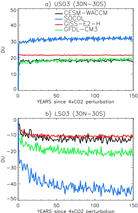
column ozone. First, we integrate over the whole col-umn to yield the total colcol-umn ozone in Dobson units (DU) (named hereafter ‘‘TO3’’). Then, we repeat the integration for the troposphere only (‘‘TRO3’’). In the stratosphere, the existence of opposite responses (see Fig. 4) motivates separating two distinct regions: the lower stratosphere, defined as the atmospheric layer between the tropopause and 20 hPa (‘‘LSO3’’), and upper stratosphere, defined as the layer between 20 hPa and 1 hPa (‘‘USO3’’). Figure 5 shows the latitudinal structure of the equilibrium response of TO3, TRO3, LSO3, and USO3 (Figs. 5a–d, respectively) to a qua-drupling of CO2.

Starting fromFig. 5a, we see that all models project a total column ozone increase at high latitudes, with a larger increase in the NH than in the SH (Fig. 5a). On the other hand, tropical column ozone responses are small. This pattern is consistent with the response in the most extreme RCP8.5 scenario (cf.Butler et al. 2016, Fig. 1 therein), despite the very different forcings em-ployed here. Most importantly, the stratospheric ozone response is the dominant contributor to the latitudinal pattern of TO3 (Figs. 5c,d). Further, we can see a large

cancellation between USO3 increases (Fig. 5c) and LSO3 decreases (Fig. 5d), resulting in a small TO3 response in the tropics (Fig. 5a). The tropospheric column ozone re-sponse is generally small (less than 5 DU), which is pos-sibly due to cancellations between ozone increase in the middle troposphere, and decrease near the tropopause in Fig. 2. In USO3, all models show a similar increase of 20 DU, with the exception of SOCOL, which shows larger values (30–35 DU) because of the lower altitude of the upper-stratospheric peak inFig. 4(and hence larger effect on ozone number density).

We also note a significant intermodel spread in the magnitude of high-latitude ozone increase, and in the sign of the response in tropical ozone column: this spread is almost entirely generated in the LSO3 (Fig. 5d). At high latitudes, the ozone increase is largest in GISS-E2-H (50 DU), and smallest in SOCOL (10– 20 DU). In the tropics, the models with the largest LSO3 decrease also exhibit a TO3 decrease; this is the case for SOCOL and GFDL CM3. This suggests that the un-certainty in the sign of the tropical TO3 response (Fig. 5a) is mostly due to uncertainty in the magnitude of the LSO3.

FIG. 5. Zonal-average column ozone response to 43CO2; (a) total, (b) tropospheric, (c) lower-stratosphere, and (d) upper-stratosphere

It is widely believed that the projected changes in LSO3 are due to the acceleration of the BDC over the twenty-first century (Butchart 2014). Thus, a possible source of spread in the tropical ozone is stratospheric upwelling. Ideally the BDC would be diagnosed using the transformed Eulerian-mean (TEM) winds (Andrews et al. 1987). Here, we calculate upwelling at the 100-hPa level, as the Eulerian-mean velocity field w averaged between turnaround latitudes (228N–228S) at the 100-hPa level resembles the TEM residual velocities [see chapter 3 inAndrews et al. (1987)]. Thus,wat this level provides an approximate measure of the strength of the up-welling branch of the BDC. The scatterplot of ozone and upwelling responses at 100 hPa is shown inFig. 6 for total (Fig. 6a) and lower-stratospheric column ozone (Fig. 6b). The negative correlation between changes in upwelling and ozone is highly significant, indicating that models with the largest upwelling re-sponse to 43CO2forcing (SOCOL and GFDL CM3) also project the largest decrease in lower-stratospheric column ozone (Fig. 6b), showing the importance of the BDC in determining the ozone response in the TLS. Similar results are obtained using w at 70 hPa (not shown). The decrease in lower-stratospheric ozone in

SOCOL and GFDL CM3 is sufficiently large to over-compensate the increase in upper-stratospheric ozone (USO3), thus resulting in a negative change in total column ozone (Fig. 5a). We thus conclude that the uncertainty in the sign of the tropical ozone response stems from the intermodel spread in the strengthening of the ascending branch of the BDC.

Interestingly, models with the largest upwelling re-sponse, such as SOCOL and GFDL CM3, are also the models with the largest tropical tropospheric warming (Fig. 3). A close relationship between tropospheric warming rates and upwelling is also evident from the transient response in the four models (Fig. S3). This suggests a possible relationship between intermodel spread in stratospheric upwelling, decreased ozone concentrations in the TLS, and climate sensitivity. De-creased ozone in the TLS can exert a substantial radia-tive forcing (Hansen et al. 2005), which might have important implications for tropospheric climate.

Up to this point, we have looked at the equilibrium response in ozone. But what time scales are needed to reach an equilibrated state? The instantaneous qua-drupling of CO2is an idealized forcing, which allows a separation of fast and slow responses, and is thus useful to elucidate the mechanisms driving the oppositely signed responses in USO3 and LSO3.Figure 7shows the time series of the response in tropical averaged USO3 (Fig. 7a) and LSO3 (Fig. 7b). The USO3 increase occurs instantaneously upon quadrupling CO2concentrations, while most of the LSO3 decrease takes place over the first 2–3 decades. This behavior clearly hints at very different processes driving the two responses, which are discussed next.

In the upper stratosphere, all models show similar cooling of up to 16 K at 1 hPa (seeFig. 3): this radiatively induced cooling occurs instantaneously upon increasing CO2(not shown), changing the reaction rates involved in the Chapman cycle, resulting in increased ozone concentrations (Haigh and Pyle 1982; Jonsson et al. 2004). On the other hand, decreased lower-stratospheric ozone concentrations are associated with enhanced up-welling (Shepherd 2008). It has been suggested that changes in upwelling occur in response to a strength-ening of the upper flanks of the subtropical jets, which pushes the critical layers upward, allowing more wave activity to penetrate into the subtropical lower stratosphere (Shepherd and McLandress 2011). The strengthening of the subtropical jets is caused by warming in the upper tropical troposphere, which is in turn a result of changes in convection and thus tropo-spheric lapse rate. Tropical stratotropo-spheric upwelling is tightly coupled with the evolution of upper-tropospheric temperature (Fig. S3). Hence, ozone changes in the TLS

FIG. 6. Scatterplot of upward velocity (w) change at 100 hPa in response to 43CO2and (a) total column ozone, and (b)

proceed at a slower pace than changes in the upper stratosphere, where ozone is mostly in photochemical equilibrium and where the concentrations are governed primarily by (fast) gas-phase reactions that are tem-perature dependent (Sander et al. 2006).

Another way of splitting fast and slow responses would be to compare ocean-coupled with atmosphere-only simulations using fixed SSTs. Unfortunately, these runs are only available for CESM(WACCM), but not for the other three models. In CESM(WACCM), we find an ozone increase in the upper stratosphere, which closely resembles that observed at 40–50 km inFig. 2a (not shown). On the other hand, the ozone decrease in the TLS region is about 10% and thus much weaker than in the coupled runs, confirming the role of surface warming and the consequent BDC strengthening in driving the ozone response in this region.

In summary, these results suggest that the tropical ozone response to 43CO2 exhibits two different

regimes: a fast response in the upper stratosphere, which is radiatively controlled via changes in gas-phase chemistry, and a slower—and opposite—response in the lower stratosphere, where ozone is dynamically controlled. This is consistent with the lifetime of ozone in both regions, which is mostly determined by photo-chemistry in the upper stratosphere, and transport be-low 20 hPa (Brasseur and Solomon 2005). Thus, the same processes that determine the background ozone distribution are also key in driving its response to 43CO2.

Ozone responses in the TLS are tied to tropospheric temperature, and are thus consistent with the definition of ‘‘feedback.’’ On the other hand, responses in the upper stratosphere are almost instantaneous and are less dependent on tropospheric temperature, thus contrib-uting to ‘‘fast adjustments’’ of the atmosphere upon quadrupling CO2. The net radiative effect depends on the combination of both, and the radiative efficiency of ozone in the two different stratospheric regions: this will be studied in a follow-up paper.

c. Seasonal and spatial distribution of the total column ozone response

The seasonal cycle of the total column ozone (TCO) response to 43CO2 in each of the CCMs is shown in Fig. 8. In the tropics, TCO responses are small, and show relatively little seasonality. On the other hand, the re-sponse at high latitudes is more seasonally dependent. In the NH, there is a distinct TCO increase that peaks in boreal late winter and spring (MAM): this is robust across the models. In the SH, we find a larger model spread in the seasonality, magnitude, and latitudinal position of the peak response, although models are generally consistent in simulating a peak increase around winter (JJA) and spring (SON), and a maximum centered around midlatitudes (608S) rather than in the high latitudes, with the exception of the GISS-E2-H model.

Next, we examine the spatial distribution of the TCO response to 43CO2. The climatological TCO distribu-tion at high latitudes is known to be zonally asymmetric (Gabriel et al. 2011), especially in the SH (Agosta and Canziani 2011;Grytsai et al. 2007). Here, we show that its response to 43CO2at high latitudes is also zonally asymmetric, as seen inFig. 9. In the SH, there is a dis-tinct peak at 608S over the Pacific sector: this localized peak stands out in all models, and is largest in the GFDL CM3 model. In the NH, there are indications of a larger ozone increase over the North Pacific, but responses are more zonally symmetric than in the SH.

Given the inhomogeneity in the spatial distribution of the TCO response, it is of interest to bring out the zonal

asymmetries in the response. This is done by plotting the deviation from the zonal-mean TCO at each latitude. To highlight the asymmetries, we average TCO over the months of the year with the maximum response for each hemisphere according toFig. 8: MAM in the NH, and JJASON in the SH (note that the peak in the SH re-sponse spans over both austral winter and spring, and this is why a longer averaging period is used for the SH). The results are shown for the SH inFig. 10, and for the NH inFig. 11. A clear wave-1 structure can be seen in the SH, with a positive lobe over the Pacific, and nega-tive over the Indian Ocean (Fig. 10). This pattern is statistically significant and robust across models, al-though the exact location and magnitude of the maxima varies strongly among models. Note that asymmetries in SOCOL and GFDL CM3 can be as large as 40%–50% of their zonal-mean response (40–70 DU). In the NH, asymmetries are generally smaller and not robust (Fig. 11). A separate analysis reveals that the asymme-tries in the SH are mostly generated in the lower stratosphere (20–100 hPa), approximately 10–20 years after quadrupling CO2, indicating that both changes in gas-phase chemistry and transport likely play an im-portant role in creating these patterns. A detailed

physical attribution of these asymmetries is outside of the scope of the present paper, and will be a subject of future work.

Taken together, these results suggest that the high-latitude ozone response to 43CO2has a distinct season-ality in both hemispheres, consistent with the effects of enhanced poleward transport of stratospheric ozone by the BDC, whose contribution is expected to be largest in winter and spring in each hemisphere (Shepherd 2008). The existence of large asymmetries around the vortex edge has been documented for Antarctic ozone depletion (Crook et al. 2008). Here, we show that ozone asymme-tries can also arise from 43CO2forcing, in the absence of halocarbon forcing and heterogeneous chemistry in polar stratospheric clouds. Longitudinal asymmetries are not taken into account in the production of ozone forcing datasets for models without interactive chemistry (Cionni et al. 2011): thus, a significant fraction of the ozone re-sponse to CO2would be missed in the SH, since asym-metries of this magnitude are known to affect the circulation, as was documented for the ozone hole (Waugh et al. 2009;Gillett et al. 2009). A follow-up study will carefully assess the effects of these asymmetries on the circulation response to 43CO2.

4. Discussion and conclusions

We have investigated the response of ozone to an abrupt quadrupling of CO2in four different CCMs. The main results are as follows:

d A robust pattern of decreased stratospheric ozone concentrations is found in the TLS region, juxtaposed to a robust increase elsewhere in the stratosphere. Tropospheric responses are comparatively small.

d In the tropics, the TCO response is small. This is due to a large cancellation between decreased ozone concentrations in the tropical lower stratosphere, and increased concentrations aloft.

d These responses occur on very different time scales: the upper-level ozone increase is a nearly instantaneous re-sponse upon quadrupling CO2, whereas the decrease in lower-stratospheric ozone occurs on decadal time scales.

d These different time scales are due to different pro-cesses controlling the stratospheric ozone responses to CO2: gas-phase chemistry dominates the response in the upper levels, while transport (tied to troposphere-surface warming) drives the response in the tropical lower stratosphere.

d The intermodel spread in the TCO response is significant, and mostly originates in the lower strato-sphere. Intermodel differences in the upwelling response to CO2 are largely responsible for differ-ences in the simulated tropical lower-stratospheric ozone decrease.

d All models show a TCO increase in the high latitudes, which maximizes in the winter–spring season of each hemisphere. In the SH, the TCO response is found to be longitudinally asymmetric.

Despite similarities in the overall stratospheric pat-tern, the ozone response to 43CO2presented here bears some differences with respect to the ozone recovery scenarios following from the Montreal Protocol docu-mented in Oman et al. (2010), Eyring et al. (2013), Iglesias-Suarez et al. (2016), and Butler et al. (2016). First, we find a larger ozone response to CO2in the NH in high latitudes, while ozone recovery is largest in the SH. Second, tropospheric column ozone changes in response to 43CO2 are virtually negligible (Fig. 5b), while they are positive and close to 10–15 DU in recovery scenarios (cf. Eyring et al. 2013, Table 4). These differences are due to the absence of

ODS trends, and of tropospheric ozone precursors in the 43CO2experiments examined here: this is a key difference between ozone recovery scenarios and the simulations presented here.

One important caveat in the present study is that the model simulations exclude the effects of ODSs, which are fixed at PI levels in both control and 43CO2 in-tegrations. In a ‘‘present day’’ atmosphere with large chlorine levels, CO2-induced stratospheric cooling could enhance Antarctic ozone depletion due to heteroge-neous chemistry. This would counteract the (positive) contribution of BDC and gas-phase chemistry, possibly leading to small high-latitude ozone responses. Further

work is needed to explore the dependency of the ozone response to CO2in present-day values of ODS concen-trations. However, we here use the PI ‘‘reference state,’’ since it is the canonical approach in studies aimed at evaluating climate feedbacks (Gregory and Webb 2008; Andrews et al. 2012).

Ozone changes in response to CO2 represent a chemistry–climate feedback. To incorporate this feed-back in climate models without interactive chemistry, it is necessary to assess the ozone response in CCMs. The magnitude of this feedback in CCMs is uncertain (Marsh et al. 2016), and the role of ozone in originat-ing this spread remains unclear. A key region for the

radiative feedback from stratospheric ozone is the TLS because of the large radiative effect of perturbations in the cold-trap region (Hansen et al. 2005;Nowack et al. 2015). The magnitude of ozone decrease induced by BDC strengthening is model dependent, and the spread in upwelling is partly related to the rate of tropospheric warming (Fig. S3). This implies that models with larger sensitivity tend to project larger ozone decreases, and may thus incorporate a larger radiative feedback from stratospheric ozone. Another pathway whereby ozone chemistry feedbacks can operate is via changes in the tropospheric circulation, such as an equatorward shift of the midlatitude jet (Chiodo and Polvani 2017) and possibly a strengthening of the Walker circulation

(Nowack et al. 2017). A follow-up study will carefully assess the radiative and dynamical feedbacks induced by ozone on the modeled climate response to CO2.

Acknowledgments.This work is supported by a grant from the U.S. National Science Foundation to Columbia University. William T. Ball was funded by the SNSF project 163206 (SIMA). The CESM(WACCM) integra-tions were performed at the National Center for Atmo-spheric Research (NCAR), which is sponsored by the U.S. National Science Foundation. All the simulation data can be obtained by request to author G.C. We acknowledge the World Climate Research Programme’s Working Group on Coupled Modelling, which is responsible for

CMIP5, and we thank the climate modeling groups for producing and making available their model output.

REFERENCES

Agosta, E. A., and P. O. Canziani, 2011: Austral spring stratospheric and tropospheric circulation interannual variability.J. Climate,

24, 2629–2647,https://doi.org/10.1175/2010JCLI3418.1. Andrews, D. G., J. R. Holton, and C. B. Leovy, 1987:Middle

At-mosphere Dynamics. International Geophysics Series, Vol. 40, Academic Press, 489 pp.

Andrews, T., J. M. Gregory, M. J. Webb, and K. E. Taylor, 2012: Forcing, feedbacks and climate sensitivity in CMIP5 coupled atmosphere-ocean climate models.Geophys. Res. Lett.,39, L09712,https://doi.org/10.1029/2012GL051607.

Austin, J., and R. J. Wilson, 2006: Ensemble simulations of the decline and recovery of stratospheric ozone.J. Geophys. Res.,

111, D16314,https://doi.org/10.1029/2005JD006907.

Banerjee, A., A. T. Archibald, A. C. Maycock, P. Telford, N. L. Abraham, X. Yang, P. Braesicke, and J. A. Pyle, 2014: Lightning NOx, a key chemistry–climate interaction: Im-pacts of future climate change and consequences for tropo-spheric oxidising capacity.Atmos. Chem. Phys.,14, 9871–9881, https://doi.org/10.5194/acp-14-9871-2014.

——, A. C. Maycock, A. T. Archibald, N. L. Abraham, P. Telford, P. Braesicke, and J. A. Pyle, 2016: Drivers of changes in stratospheric and tropospheric ozone between year 2000 and 2100. Atmos. Chem. Phys., 16, 2727–2746, https://doi.org/ 10.5194/acp-16-2727-2016.

Brasseur, G. P., and S. Solomon, 2005:Aeronomy of the Middle Atmosphere: Chemistry and Physics of the Stratosphere and Mesosphere. Atmospheric and Oceanic Sciences Library, Vol. 32, Kluwer Academic, 646 pp.

Butchart, N., 2014: The Brewer-Dobson circulation. Rev. Geo-phys.,52, 157–184,https://doi.org/10.1002/2013RG000448. Butler, A. H., J. S. Daniel, R. W. Portmann, A. R. Ravishankara,

P. J. Young, D. W. Fahey, and K. H. Rosenlof, 2016: Diverse policy implications for future ozone and surface UV in a changing climate.Environ. Res. Lett.,11, 064017,https://doi.org/ 10.1088/1748-9326/11/6/064017.

Charlton-Perez, A. J., and Coauthors, 2013: On the lack of strato-spheric dynamical variability in low-top versions of the CMIP5 models.J. Geophys. Res. Atmos.,118, 2494–2505,https://doi.org/ 10.1002/jgrd.50125.

Chiodo, G., and L. M. Polvani, 2016: Reduction of climate sensitivity to solar forcing due to stratospheric ozone feedback.J. Climate,

29, 4651–4663,https://doi.org/10.1175/JCLI-D-15-0721.1. ——, and ——, 2017: Reduced Southern Hemispheric circulation

response to quadrupled CO2 due to stratospheric ozone

feedback. Geophys. Res. Lett.,44, 465–474, https://doi.org/ 10.1002/2016GL071011.

Cionni, I., and Coauthors, 2011: Ozone database in support of CMIP5 simulations: Results and corresponding radiative forcing.Atmos. Chem. Phys.,11, 11 267–11 292,https://doi.org/ 10.5194/acp-11-11267-2011.

Crook, J. A., N. P. Gillett, and S. P. E. Keeley, 2008: Sensitivity of Southern Hemisphere climate to zonal asymmetry in ozone. Geophys. Res. Lett., 35, L07806, https://doi.org/10.1029/ 2007GL032698.

Dessler, A. E., M. R. Schoeberl, T. Wang, S. M. Davis, and K. H. Rosenlof, 2013: Stratospheric water vapor feedback. Proc. Natl. Acad. Sci. USA,110, 18 087–18 091,https://doi.org/ 10.1073/pnas.1310344110.

Dietm_üller, S., M. Ponater, and R. Sausen, 2014: Interactive ozone induces a negative feedback in CO2-driven climate change

simulations.J. Geophys. Res. Atmos.,119, 1796–1805,https:// doi.org/10.1002/2013JD020575.

Donner, L. J., and Coauthors, 2011: The dynamical core, physical parameterizations, and basic simulation characteristics of the atmospheric component AM3 of the GFDL global coupled model CM3.J. Climate,24, 3484–3519,https://doi.org/10.1175/ 2011JCLI3955.1.

Eyring, V., and Coauthors, 2010: Multi-model assessment of stratospheric ozone return dates and ozone recovery in CCMVal-2 models.Atmos. Chem. Phys.,10, 9451–9472,https:// doi.org/10.5194/acp-10-9451-2010.

——, and Coauthors, 2013: Long-term ozone changes and associ-ated climate impacts in CMIP5 simulations.J. Geophys. Res. Atmos.,118, 5029–5060,https://doi.org/10.1002/jgrd.50316. Forster, P. M., T. Andrews, P. Good, J. M. Gregory, L. S. Jackson, and

M. Zelinka, 2013: Evaluating adjusted forcing and model spread for historical and future scenarios in the CMIP5 generation of climate models.J. Geophys. Res. Atmos.,118, 1139–1150,https:// doi.org/10.1002/jgrd.50174.

Gabriel, A., H. Körnich, S. Lossow, D. H. W. Peters, J. Urban, and D. Murtagh, 2011: Zonal asymmetries in middle atmospheric ozone and water vapour derived from Odin satellite data 2001– 2010. Atmos. Chem. Phys., 11, 9865–9885, https://doi.org/ 10.5194/acp-11-9865-2011.

Garcia, R. R., and W. J. Randel, 2008: Acceleration of the Brewer– Dobson circulation due to increases in greenhouse gases.J. Atmos. Sci.,65, 2731–2739,https://doi.org/10.1175/2008JAS2712.1. Garny, H., V. Grewe, M. Dameris, G. E. Bodeker, and A. Stenke, 2011:

Attribution of ozone changes to dynamical and chemical processes in CCMs and CTMs.Geosci. Model Dev.,4, 271–286,https:// doi.org/10.5194/gmd-4-271-2011.

Gillett, N. P., J. F. Scinocca, D. A. Plummer, and M. C. Reader, 2009: Sensitivity of climate to dynamically-consistent zonal asymmetries in ozone.Geophys. Res. Lett.,36, L10809,https:// doi.org/10.1029/2009GL037246.

Gregory, J., and M. Webb, 2008: Tropospheric adjustment induces a cloud component in CO2forcing.J. Climate,21, 58–71,https://

doi.org/10.1175/2007JCLI1834.1.

Griffies, S. M., and Coauthors, 2005: Formulation of an ocean model for global climate simulations.Ocean Sci.,1, 45–79,https://doi.org/ 10.5194/os-1-45-2005.

Grise, K. M., and L. M. Polvani, 2014: Is climate sensitivity related to dynamical sensitivity? A Southern Hemisphere perspective. Geophys. Res. Lett., 41, 534–540, https://doi.org/10.1002/ 2013GL058466.

Grytsai, A. V., O. M. Evtushevsky, O. V. Agapitov, A. R. Klekociuk, and G. P. Milinevsky, 2007: Structure and long-term change in the zonal asymmetry in Antarctic total ozone during spring.Ann. Geophys.,25, 361–374,https://doi.org/10.5194/angeo-25-361-2007. Haigh, J. D., and J. A. Pyle, 1982: Ozone perturbation experiments in a two-dimensional circulation model.Quart. J. Roy. Meteor. Soc.,108, 551–574,https://doi.org/10.1002/qj.49710845705. Hansen, J., and Coauthors, 2005: Efficacy of climate forcings.J. Geophys.

Res.,110, D18104,https://doi.org/10.1029/2005JD005776. Hegglin, M. I., and T. G. Shepherd, 2009: Large climate-induced changes

in ultraviolet index and stratosphere-to-troposphere ozone flux. Nat. Geosci.,2, 687–691,https://doi.org/10.1038/ngeo604. Horowitz, L. W., and Coauthors, 2003: A global simulation of

Iglesias-Suarez, F., P. J. Young, and O. Wild, 2016: Stratospheric ozone change and related climate impacts over 1850–2100 as modelled by the ACCMIP ensemble.Atmos. Chem. Phys.,16, 343–363,https://doi.org/10.5194/acp-16-343-2016.

Isaksen, I. S. A., and Coauthors, 2009: Atmospheric composition change: Climate–chemistry interactions.Atmos. Environ.,43, 5138–5192,https://doi.org/10.1016/j.atmosenv.2009.08.003. Jonsson, A. I., J. de Grandpré, V. I. Fomichev, J. C. McConnell, and

S. R. Beagley, 2004: Doubled CO2-induced cooling in the

middle atmosphere: Photochemical analysis of the ozone radi-ative feedback.J. Geophys. Res.,109, D24103,https://doi.org/ 10.1029/2004JD005093.

Kinnison, D. E., and Coauthors, 2007: Sensitivity of chemical tracers to meteorological parameters in the MOZART-3 chemical transport model.J. Geophys. Res.,112, D20302,https://doi.org/ 10.1029/2006JD007879.

Lacis, A. A., D. J. Wuebbles, and J. A. Logan, 1990: Radiative forcing of climate by changes in the vertical distribution of ozone.J. Geophys. Res.,95, 9971–9981,https://doi.org/10.1029/ JD095iD07p09971.

Langematz, U., S. Meul, K. Grunow, E. Romanowsky, S. Oberl_änder, J. Abalichin, and A. Kubin, 2014: Future Arctic temperature and ozone: The role of stratospheric composition changes.J. Geophys. Res. Atmos.,119, 2092–2112,https://doi.org/10.1002/2013JD021100. Marsh, D. R., M. J. Mills, D. E. Kinnison, J.-F. Lamarque, N. Calvo, and L. M. Polvani, 2013: Climate change from 1850 to 2005 sim-ulated in CESM1 (WACCM).J. Climate,26, 7372–7391,https:// doi.org/10.1175/JCLI-D-12-00558.1.

——, J.-F. Lamarque, A. J. Conley, and L. M. Polvani, 2016: Strato-spheric ozone chemistry feedbacks are not critical for the de-termination of climate sensitivity in CESM1 (WACCM).Geophys. Res. Lett.,43, 3928–3934,https://doi.org/10.1002/2016GL068344. Meul, S., U. Langematz, S. Oberländer, H. Garny, and P. Jöckel, 2014:

Chemical contribution to future tropical ozone change in the lower stratosphere.Atmos. Chem. Phys.,14, 2959–2971,https:// doi.org/10.5194/acp-14-2959-2014.

——, S. Oberl_änder-Hayn, J. Abalichin, and U. Langematz, 2015: Nonlinear response of modelled stratospheric ozone to changes in greenhouse gases and ozone depleting substances in the recent past.Atmos. Chem. Phys.,15, 6897–6911,https:// doi.org/10.5194/acp-15-6897-2015.

Muthers, S., and Coauthors, 2014: The coupled atmosphere– chemistry–ocean model SOCOL-MPIOM. Geosci. Model Dev.,7, 2157–2179,https://doi.org/10.5194/gmd-7-2157-2014. ——, C. C. Raible, E. Rozanov, and T. F. Stocker, 2016: Response of the

AMOC to reduced solar radiation—The modulating role of at-mospheric chemistry.Earth Syst. Dyn.,7, 877–892,https://doi.org/ 10.5194/esd-7-877-2016.

Myhre, G., and Coauthors, 2013: Anthropogenic and natural radi-ative forcing.Climate Change 2013: The Physical Science Basis, T. F. Stocker et al., Eds., Cambridge University Press, 659–740. Noda, S., and Coauthors, 2017: Impact of interactive chemistry of stratospheric ozone on Southern Hemisphere paleoclimate simulation.J. Geophys. Res. Atmos.,122, 878–895,https:// doi.org/10.1002/2016JD025508.

Nowack, P. J., N. L. Abraham, A. C. Maycock, P. Braesicke, J. M. Gregory, M. M. Joshi, A. Osprey, and J. A. Pyle, 2015: A large ozone-circulation feedback and its implications for global warming assessments.Nat. Climate Change,5, 41–45, https://doi.org/10.1038/nclimate2451.

——, P. Braesicke, N. L. Abraham, and J. A. Pyle, 2017: On the role of ozone feedback in the ENSO amplitude response un-der global warming. Geophys. Res. Lett., 44, 3858–3866, https://doi.org/10.1002/2016GL072418.

Oman, L. D., and Coauthors, 2010: Multimodel assessment of the factors driving stratospheric ozone evolution over the 21st century. J. Geophys. Res., 115, D24306, https://doi.org/ 10.1029/2010JD014362.

Revell, L. E., G. E. Bodeker, P. E. Huck, B. E. Williamson, and E. Rozanov, 2012: The sensitivity of stratospheric ozone changes through the 21st century to N2O and CH4.Atmos.

Chem. Phys.,12, 11 309–11 317, https://doi.org/10.5194/acp-12-11309-2012.

Sander, S. P., and Coauthors, 2006: Chemical kinetics and photo-chemical data for use in atmospheric studies, evaluation num-ber 15. NASA Jet Propulsion Laboratory Publ. 06-2, 523 pp. Schmidt, G. A., and Coauthors, 2014: Configuration and

assess-ment of the GISS ModelE2 contributions to the CMIP5 ar-chive.J. Adv. Model. Earth Syst.,6, 141–184,https://doi.org/ 10.1002/2013MS000265.

Shepherd, T. G., 2008: Dynamics, stratospheric ozone, and climate change. Atmos.–Ocean,46, 117–138, https://doi.org/10.3137/ ao.460106.

——, and C. McLandress, 2011: A robust mechanism for strengthening of the Brewer–Dobson circulation in response to climate change: Critical-layer control of subtropical wave breaking.J. Atmos. Sci.,68, 784–797,https://doi.org/10.1175/ 2010JAS3608.1.

Shindell, D. T., and Coauthors, 2013: Interactive ozone and methane chemistry in GISS-E2 historical and future climate simulations.Atmos. Chem. Phys.,13, 2653–2689,https://doi.org/ 10.5194/acp-13-2653-2013.

Shine, K. P., and Coauthors, 2003: A comparison of model-simulated trends in stratospheric temperatures.Quart. J. Roy. Meteor. Soc.,129, 1565–1588,https://doi.org/10.1256/qj.02.186. Stenke, A., M. Schraner, E. Rozanov, T. Egorova, B. Luo, and

T. Peter, 2013: The SOCOL version 3.0 chemistry–climate model: Description, evaluation, and implications from an ad-vanced transport algorithm.Geosci. Model Dev.,6, 1407–1427, https://doi.org/10.5194/gmd-6-1407-2013.

Taylor, K. E., R. J. Stouffer, and G. A. Meehl, 2012: An overview of CMIP5 and the experiment design.Bull. Amer. Meteor. Soc.,

93, 485–498,https://doi.org/10.1175/BAMS-D-11-00094.1. Waugh, D. W., L. Oman, P. A. Newman, R. S. Stolarski, S. Pawson,

J. E. Nielsen, and J. Perlwitz, 2009: Effect of zonal asymme-tries in stratospheric ozone on simulated Southern Hemi-sphere climate trends.Geophys. Res. Lett.,36, L18701,https:// doi.org/10.1029/2009GL040419.

WMO, 1992: Scientific assessment of ozone depletion: 1991. WMO/TD-25, 327 pp.,https://acd-ext.gsfc.nasa.gov/Documents/ O3_Assessments/Docs/WMO_UNEP_1991.pdf.

——, 2014: Scientific assessment of ozone depletion: 2014. WMO/TD-55, 416 pp.,http://www.wmo.int/pages/prog/arep/gaw/ozone_2014/ documents/Full_report_2014_Ozone_Assessment.pdf. Zubov, V., E. Rozanov, T. Egorova, I. Karol, and W. Schmutz,