Place du Congrès 1 B-1000 Brussels Tel: (32.2) 229.39.11 Fax: (32.2) 219.41.51 VAT: BE 424.123.986 e-mail: [email protected] • website: http://www.enepri.org
E
UROPEAN
N
ETWORK OF
E
CONOMIC
P
OLICY
R
ESEARCH
I
NSTITUTES
W
ORKINGP
APERN
O. 15/O
CTOBER2002
E
STIMATING THE
E
FFECTS OF
F
ISCAL
P
OLICY
IN
OECD C
OUNTRIES
ROBERTO PEROTTI
CEPS Working Documents are published to give an indication of the work within CEPS’ various research programmes and to stimulate reactions from other experts in the field. Unless otherwise indicated, the views expressed are attributable only to the author in a personal capacity and not to any institution with which he is associated.
ISBN 92-9079-402-X
Available for free downloading from the CEPS website (http://www.ceps.be)
Estimating the e
ff
ects of
fi
scal policy in
OECD countries
Roberto Perotti
∗First version: June 2002
This revision: September 2002
Abstract
This paper studies the effects of fiscal policy on GDP, prices and
interest rates in 5 OECD countries, using a structural Vector
Autore-gression approach. Its main results can be summarized as follows: 1)
The estimated effects of fiscal policy on GDP tend to be small:
pos-itive government spending multipliers larger than 1 tend to be the
exception; 2) The effects of fiscal policy on GDP and its components
have become substantially weaker over time; 3) Under plausible values
of the price elasticity, government spending has positive effects on the
price level, although usually small; 4) Government spending shocks
have significant effects on the nominal and real short interest rate,
but of varying signs; 5) In the post-1980 period, net tax shocks have
positive short run effects on the nominal interest rate, and typically
negative or zero effects on prices; 6) The US is an outlier in many
dimensions; responses to fiscal shocks estimated on US data are
of-ten not representative of the average OECD country included in this sample.
∗European University Institute and Centre for Economic Policy Research. This paper
Estimating the e
ff
ects of
fi
scal policy
in OECD countries
Roberto Perotti
1
Introduction
While most economists would agree that an exogenous 10 percent increase
in money supply will lead to some increase in prices after a while, perfectly
reasonable economists can and do disagree even on thesignof the response of
private consumption or private investment to an exogenous shock to govern-ment purchases of goods. Yet, there is no doubt that many more resources
have been devoted to the study of monetary policy than fiscal policy; only
recently has a small but growing literature emerged that applies to fiscal
policy time series methods that have long been standard in the analysis of
monetary policy.1
One reason why relatively little empirical work has been done on the
effects of fiscal policy is probably the difficulty in assembling the necessary
data at high enough frequency and over sufficiently long periods. In this
paper, I present evidence on the effects of fiscal policy in five countries for
which I was able to assemble sufficiently detailed quarterly data on the budget
of the general government: the US, West Germany, the UK, Canada, and Australia. I do so using an approach originally developed in Blanchard and
Perotti [2002]: in essence, the method exploits institutional features of fiscal
policymaking and detailed information on the automatic effects of GDP and
inflation on tax revenues and government spending to identify the exogenous
fiscal policy shocks in a structural vector autoregression.
Beside including more countries, this paper extends the methodology of
Blanchard and Perotti [2002] to study the interaction offiscal and monetary
policy, and the effects of fiscal policy on prices. Recent developments both
in the theory and in the practice of monetary policy have also emphasized
the link between fiscal and monetary policy. At the policy level, many of
the institutional provisions of the EMU have been rationalized in terms of
constraints onfiscal policy to enable monetary policy to achieve its mandate
1I review this literature in the next section. Almost all the recent empirical literature
refers to the United States.The exceptions known to me are Favero [2002] and Marcellino [2002], who estimatefiscal policy VARs using half-yearly data from four European coun-tries: France, Italy, Spain, and Germany.
of price stability. And several policy measures, like the EU Council of
Min-isters’s reprimand against Ireland in February 2001, have been motivated by
the alleged affects of specific fiscal policy actions on inflation and interest
rates. At the academic level, research on the Taylor rule has inevitably run
into the issue of how fiscal policy might interfere with interest rate control
(see Taylor [1996], Taylor [2000], and Woodford [1999]); more generally, the
fiscal theory of the price level has emphasized the potential links between
fiscal policy and the price level (see, among others, Cochrane [2001], Sims
[1994] and [1999], and Woodford [2001]).2
The main conclusions of the analysis can be summarized as follows: 1)
The estimated effects of fiscal policy on GDP tend to be small: positive
government spending multipliers larger than 1tend to be the exception; the
tax multipliers are usually negative but even smaller in absoulte value; 2) The
effects offiscal policy on GDP and its components have become substantially
weaker over time: in the post-1980 period significantly negative multipliers of
government spending are the norm; the negative effects of taxation have also
become weaker; 3) To understand the effects of fiscal policy on prices, the
price elasticity of the government budget items is crucial, an issue that has not been widely appreciated. Once Once plausible values of the price elasticity
of government spending are imposed, the negative effects of government
spending on prices that have been frequently estimated become positive,
although usually small and not always significant; 4) Government spending
shocks have significant effects on the nominal and real short interest rate,
but of varying signs: in the post-1980 period, after 4 quarters the effect is
positive in three countries, negative in two; 5) In the post-1980 period, net
tax shocks have positive short run effects on the nominal interest rate, and
typically negative or zero effects on prices; 6) The US is an outlier in many
dimensions; responses to fiscal shocks estimated on US data are often not
representative of the average OECD country included in this sample.3
The plan of the paper is as follows. Section 2 briefly reviews alternative
approaches that have been used to identify fiscal shocks in VARs and the
methodology I use. Section 3 describes the data and how the elasticities of government spending and taxes to economic activity are constructed.
Sec-tion 4 briefly discusses a few diagnostic checks on the estimated VARs. The
2The evidence presented in this paper, however, has nothing to say on thefiscal theory
of the price level. By its nature, the theory places no testable restriction on the observed relation betweenfiscal variables and the price level.
3It is well understood, but still worth repeating, that the results presented here have
estimated effects of government spending on GDP and the short interest rate
are presented in Section 5. Section 6 discusses the effects of government
spending shocks on GDP components. Section 7 discusses the rationale for and consequences of including interest rates in the VAR. Section 8 presents the price responses to government spending shocks. Section 9 displays the
results of a tax shock on GDP, interest rate and prices. Section 10
con-cludes. An appendix provides further details on the construction of the tax elasticities.
2
The
fi
scal shocks
2.1
Approaches to identi
fi
cation
A small but growing literature has recently applied VAR methods to the
analysis of fiscal policy In this section, I briefly review the four different
approaches to identification of fiscal policy shocks that have been used.4
(i) In a first group, represented by Burnside, Eichenbaum and Fisher
[2001], Christiano, Eichenbaum and Eidelberg [1999] , and Ramey and Shapiro
[1998], fiscal policy shocks are identified by way of the “narrative approach”
of Romer and Romer [1989]. All these papers trace the effects of a dummy
variable capturing the “Ramey and Shapiro” fiscal episodes: the Korean war
military buildup, the Vietnam war buildup, and the Reaganfiscal expansion.
The advantages and disadvantages of this approach are well known. If these episodes are truly exogenous and unanticipated, and one is only
inter-ested in estimating their effects, there is no need to impose other potentially
controversial identifying assumptions: all is needed is a reduced form regres-sion. But the approach might run into two types of problems. First, these
episodes might not be entirely unanticipated. Second, other substantialfiscal
shocks, of different type or sign, might have occurred around the same time,
thus polluting the identification of the fiscal shocks.5
(ii) A second approach, represented by Mountford and Uhlig [2002],
con-sists in identifyingfiscal shocks by sign restrictions on the impulse responses,
following a methodology originally applied by Uhlig [1997] and Faust [1998]
4This brief review is based on the papers known to me at the time of writing. I apologize
for involuntary omissions of relevant contributions.
5For instance, Ramey and Shapiro date the start of the Korean war shock in1950:3,
based on the large observed increase in military spending; but net tax revenues also in-creased by more than three standard deviations in1950:2 and1950:3; and in four quarters between 1948:2 and 1950:3, government spending increased by between two and three standard deviations. It is not obvious how to disentangle the effects of the Korean dummy variable from the delayed effects of these precedingfiscal shocks.
to monetary policy analysis. For instance, “revenue” shocks are identified by imposing that tax revenue response increases while the government spending response does not, and that all responses such that both tax revenues and GDP increase identify a business cycle shock.
An important advantage of this approach is that it is well suited to handle
anticipated fiscal shocks: the estimated effect on, say, private consumption
at time 0 could be the response to a revenue shock that occurs later. On the other hand, by identifying revenue shocks via the condition that tax revenues and output do not covary positively in response to the shock, the approach rules out by assumption a whole set of “non-keynesian” output responses to
fiscal shocks.6 A second cost of this approach is also related to its benefits:
while it can better handle anticipated fiscal policy, it cannot pin down when
thefiscal shock occurs.
(iii) A third approach, represented by Fatas and Mihov [2001] and Favero
[2002], essentially relies on Choleski ordering to identify fiscal shocks. In the
former, government spending is ordered first: in the latter, fiscal shocks are
ordered last, by analogy to monetary shocks in some recent monetary policy VAR contributions. A discussion of this approach will be implicit in the discussion of the next one.
(iv) The fourth approach, developed by Blanchard and Perotti [2002], is
akin to a structural VAR.7 Identification is achieved by exploiting decision
lags infiscal policy, and institutional information about the elasticity offiscal
variables to economic activity. In this paper, I extend this approach to take
into account interest rates and inflation.8
Consider the benchmark specification, a 5-variable VAR that includes the
following variables: the log of real government spending on goods and services
per capita gt (government spending for short), the log of real net primary
taxes per capita (defined as government revenues less government transfers,
both net of property income) tt, the log of real output per capitayt, the log
of the price level pt, and the 3-month nominal interest rate it.9 Denoting
6For some empirical evidence on non-Keynesian effects offiscal policy, see Alesina et
al. [2002], Giavazzi, Jappelli and Pagano [2000], and Perotti [1999]. Other shocks in teh Mountford and Uhlig [2002] approach, like spending shocks, are identified with a minimal set of restrictions, involving only the behavior of government spending and taxation.
7An early application of this approach is Blanchard and Watson [1986].
8At the same time as this paper was being written, Canzoneri, Cumby and Diba [2002]
also extended the Blanchard and Perotti [2002] methodology to include inflation and in-terest rate responses to the analysis of US fiscal policy. Instead of bringing in external information on the elasticities of fiscal variables to economic activity, Marcellino [2002] estimates these elasticities by specifiying a larger model with overidentifying restrictions.
9This two-way breakdown of the government budget is obviously only one of many
the vector of endogenous variables by Xt and the vector of reduced form
residuals by Ut, the reduced form VAR can be written as:
Xt=A(L)Xt−1+Ut, (1)
where Xt≡ [gt tt yt pt it]0 and Ut ≡[ugt utt u
y t u
p
t uit]0.
The reduced form residuals of thegt andtt equations, ugt and utt, can be
thought of as the sum of the automatic and discretionary shocks to govern-ment spending and net taxes, respectively. Taxes and, to a lesser degree, government spending react automatically to shocks in the other endogenous variables, for instance because of the automatic increase in tax revenues when output increases, holding constant tax rates. Taxes and government spending can also be changed in a discretionary way by the policymaker, for instance by changing the tax rates themselves. Formally, one can write the reduced form government spending and net tax residuals as
utt = αtyuyt +αtpupt +αtiuit+βtge g
t +ett (2a) ugt = αgyu
y
t +αgpu p
t +αgiuit +βgtett +e g
t (2b)
where egt and et
t are the “structural” shocks to government spending and
taxes, part of the vector of mutually uncorrelated “structural” shocks Ft ≡
[egt ett ext e p
t eit]0. The key to identification is the observation that it
typically takes longer than three months to decide a discretionary change in
fiscal policy; as a consequence, in quarterly data the coefficients α0
jks in (2)
reflect only the automatic response of fiscal variables to economic activity,
andegt andet
tcan be interpreted as the discretionary components of thefiscal
policy reduced form residuals.
Identifyingegt andett would still not be feasible if one had to estimate the
α0
jks,becausee
g
t andett are correlated with the reduced form residuals on the
rhs of (2). However, we do have independent information on theα0
jks, whose
construction is discussed in detail in the next section. With these values of
theα0
jks, one can construct linear combinations of the two structural shocks,
or the cyclically adjusted fiscal shocks:
ut,CAt ≡ u t
t−(αtyuyt +αtpupt +αtiuit) =βtge g t +e
t
t (3a) ug,CAt ≡ u
g
t −(αgyu y
t +αgpu p
t +αgiuit) =βgtett +e g
t (3b)
different effects than transfers. Summing algebraically taxes and transfers makes sense if one believes that in the short- and medium run fiscal policy operates mostly via a demand channel. In future work, I am planning to study different disaggregations of the government budgets — in particular, government consumption vs government investment, and taxes vs transfers.
There is still little guidance, theoretical or empirical, on how to sort out the
two structural shocks et
t and e g
t from the cyclically adjusted fiscal shocks.
Therefore, I compute impulse responses under the two alternative orthog-onalizations: as it turns out, in all cases the correlation between the two
cyclically adjustedfiscal shocks is low enough that the ordering of the
struc-tural shocks is immaterial to the results.10
Because both egt and et
t are orthogonal to the other structural shocks of
the economy; they can be used as instruments in the remaining equations.11
Once the structural shocks are identified, the impulse responses are
con-structed using the average elasticities over the relevant sample periods.
2.2
What are the
fi
scal shocks?
How to interpret the fiscal policy shocksett ande
g
t? Government spending is
typically budgeted in advance for the whole fiscal year, hence one could
ar-gue that thefiscal shocks identified by the methodology above are not really
unanticipated. However, the yearly budget is often mostly a political
doc-ument, whose figures typically bear little relation to the actual expenditure
eventually disbursed, and which is discounted by the private sector as such.
In addition, even if the total expenditure for the year werefixed and reliable,
actual cash disbursements can vary unpredictably on a quarterly basis for a
variety of reasons.12
More importantly, there are shocks to budgeted expenditure all through the year, due to mid-year legislation and executive decisions. Under this
interpretation, however, while as we have seen decision lags in fiscal
policy-making help identify the shocks, implementation lags contribute to policy-making them predictable.
Thus, the validity of the identification procedure outlined here is a matter
of degree. It depends on how long and predictable the decision lags are relative to the implementation lags, and on how important the yearly budget is relative to quarterly policymaking.
10Although I consider only the two Choleski orderings of the two cyclically adjusted fiscal variables, one should recognize that, lacking a theory, really anyrotationof the two shocks could be defended.
11The ordering of the remaining variables is immaterial if one is only interested in
estimating the effects of fiscal policy shocks, as it is the case in this paper. Assuming for instance that output is orderedfirst among the other variables, one can estimate the “output” equationuyt =γytut
t+γygu g t+e
y
t,usingettande g
t as instruments forutt andu g t,
and similarly for the other equations.
12Strictly speaking, thefiscal policy shock of the last quarter of thefiscal year would be
3
Speci
fi
cation, samples and data
3.1
Speci
fi
cation and samples
I estimate the VAR specification described in section 2.1on quarterly data
fromfive countries: Australia, Canada, West Germany, United Kingdom, and
Unites States.13 The benchmark VAR includes the logs of real GDP, real
government spending and real net taxes, all in per capita terms, and deflated
using the GDP deflator; the log of the GDP deflator; and the nominal 3
months interest rate (the federal funds rate for the US). All variables (except the interest rates) have been seasonally adjusted by the original sources. All equations include four lags of each endogenous variable, a constant, and no
time trends. The precise samples of the benchmark VARs are: USA: 1961:1
- 2000:4; West Germany: 1961:1- 1989:4; United Kingdom: 1964:1 - 2001:2;
Canada: 1962:1 - 2001:4; Australia: 1964:1- 2000:4.
3.2
The data
One reason why fiscal policy VARs have been less popular than their
mone-tary policy counterparts is that fiscal policy data at high enough frequency
are more difficult to collect; in most countries they simply do not exist.14
All thefiscal data used in this paper originate from only one source per
country, ensuring internal consistency;15 in all cases, the fiscal data are part
13In Blanchard and Perotti [2002], we estimated quarter dependent 3-variable VARs,
on the basis that there is some quarter dependence in tax collections. However, we also found that quarter dependence makes little difference for the US. The description of the institutional features of the tax systems in Appendix1makes clear that only for corporate income taxes in the United Kingdom is quarter dependence likely to be substantial. More-over, in the 5-variable VARs that I estimate in this paper, allowing for quarter dependence would quickly exhaust the available degrees of freedom.
14Of the other OECD countries, France, Japan and New Zealand seem to have quarterly
general government budgetfigures for long enough periods. However, it appears that parts of the budget data of these countries might be interpolated from annual figures. I am currently investigating the nature of the data for these countries.
Other countries have some quarterly or even monthly data on some parts of the budget, or covering only the central government accounts. Some commerical vendors and interna-tional organizations also have quarterly or semi-annualfigures on the general government budget of several countries, but, with the exceptions of the countries included in this paper, these are to varying extents interpolated from annualfigures.
15The sources for both thefiscal and the national income accounts data are: the NIPA
accounts from the Bureau of Economic Analysis for the US; the DIW National Accountfiles for Germany; the United Kingdom National Accounts and the Financial Statistics files, from the Office of National Statistics, for the United Kingdom; the CANSIM database of Statistics Canada for Canada; and the Australian Bureau of Statistics database for
of the integrated system of national accounts, thus ensuring consistency with other national income account data. In general, all the government budget
and national income account data follow the guidelines of the 1993 System
of National Accounts. The two fiscal variables used in the VARs, net taxes
and government spending, have been constructed from disaggregated data as follows:
Net taxes = Revenues - Transfers
Revenues = Tax revenues + Non-tax revenues
Tax revenues = Direct taxes on individuals + Direct taxes on corporation + Social security taxes + Production taxes
Non-tax revenues = Current transfers received by the general government + Net capital transfers received by the general government
Transfers: = Social security transfers to households + Other transfers to
households + Subsidies to firms + Transfers abroad
Government spending on goods and services = Government consumption + Government gross capital formation
Government gross capital formation = Gross fixed capital formation by
the government + Net acquisition of non produced non financial assets +
Change in inventories
Some sub-items have been reclassified relative to the1993 SNA definition
in order to make each item more homogeneous in terms of its output and
price elasticity. Thus, in the1993 SNA the item “Direct taxes on individuals”
includes mostly income taxes, but also property taxes, taxes on land, and poll taxes, all of which are not elastic to output contemporaneously, and
licenses and fees paid by households, which are closer to indirect taxes.16 The
item “Production taxes” includes mostly indirect taxes like VAT, but also payroll taxes, which are more akin to social security taxes, and land taxes, which also are inelastic to GDP contemporaneously. Whenever possible, I
have reclassified all revenue items that are inelastic to GDP into “Current
transfers received by the government” or “Net capital transfers received by
the government”;17 I have also reclassified payroll taxes into “Social security
Australia.
16Licenses and fees paid by businesses are included in production taxes.
17In the 1993 SNA, “Current transfers received by the government” include items such
taxes”, and licenses and fees paid by households into “Production taxes”. The item “Social security tranfers” includes unfunded pension liabilities contributions by the government; as these items also appear as social security contributions, they wash out when constructing net taxes.
The item “Government consumption” (or “Current spending on goods and services”) is net of market sales by the government and of capital con-sumption allowances, an item which is usually imprecisely measured. The item “Government gross capital formation” includes the change in
invento-ries, but often quarterly data on acquisition of non produced non-financial
assets (a very minor item) are missing.
The items “Property income received” and “Property income paid” by the government — mostly interest, but also rents and dividends from state owned enterprises — are excluded, for two reasons: there coverage tends to be spotty in quarterly data, and there are economic reasons to focus on the primary budget.
Under the guidelines of the new1993 National Income Account Systems,
all budget items should be recorded on an accrual basis. If this were in-deed the case, there would be no issue of collection lags: all taxes would be recorded at the time the corresponding liability arises. In reality, even
in the new system taxes are at most recorded on a “modified cash” basis,
which consists in adjusting for the lag between the time taxes are withheld by the employer or paid by the taxpayer and the time they are recorded by the agency in charge of collecting them.
The series cover the whole budget of the general government (central government + state and local governments + social security funds), not just a
few items. This is important because most theories postulate that the effects
of a budget item also depend on the concomitant and expected movements in the others. Covering the whole general government is also important because from the point of view of the private sector an increase in income taxes by
the local government is likely to have similar effects, to afirst approximation,
as the same increase by the central government.
Among the other data, the short interest rate is often the binding con-straint on the length of the sample. I use an interest rate as close as possible to a Central Bank instrument, provided an unbroken series is available from
the early 1960s.18
18All interest rates are expressed on an annual basis. In the benchmark specifications,
I use the Federal Funds Rate in the USA; the interest rate on three month bills for the United Kingdom (variable11260CZ,International Financial Statisticsof the International Monetary Fund); the three month interbank rate in West Germany (series IRS in the OECD Quarterly National Accounts database); the treasury bill rate in Canada (series
15660CZ,International Financial Statistics of the International Monetary Fund); and the
3.3
Constructing the output and price elasticities
The coefficients αjk’s in equation (2) are weighted averages of the elasticity
of each component of net taxes and government spending.19
Consider first the output elasticity of net taxes. The output elasticity
of each component of tax revenues is constructed from a decomposition of actual revenues into a tax rate and a tax base. Start with direct taxes on individuals, typically the largest component of tax revenues. This can be
written as:20
Ht=S(WtPt)Wt(Et)Et(Yt) (4)
whereHt is total real direct taxes on individuals,S is the tax rate,Wt is the
real wage,Pt is the GDP deflator, Etis employment, andYt is output. Thus,
WtEt is the tax base (ignoring non-labor income). Letting lower-case letters
denote logs, and totally differentiating, one obtains:
dht =
∂s ∂wt
dwt+
∂wt
∂et det+
∂et
∂yt dyt+
∂s ∂pt
dpt (5a)
=
·µ
∂s ∂wt
+ 1

∂wt
∂et
+ 1
¸
∂et
∂yt dyt+
∂s ∂pt
dpt (5b)
Thus, the term multiplying dyt in (5b) is the equivalent of αty in equation
(2a) for this particular tax revenue, and the term ∂s/∂pt is the equivalent of
αtp.
For most member countries, the OECD computes the elasticity of tax
revenues per person to average real earnings, the term ∂s/∂wt+ 1 in (5b),
using information on the tax code of each country and the distribution of
tax payers in each bracket, at intervals of a few years.21 Following Blanchard
and Perotii [2002] I then estimate the contemporaneous elasticity of the real
wage to employment, ∂wt/∂et, as the coefficient on lag 0 from a regression
of the log change in real wage on lead 1 and lags 0 to 4 of log employment
changes; and I estimate the elasticity of employment to output, ∂et/∂yt,in
a similar way.22 A similar methodology can be used to estimate the elasticity
of social security taxes to output.
interest rate on three month Treasury notes in Australia (series VNEQ.UN_RTN until decmber1997 and FIRMMTNIY3 since January1998, from the Reserve Bank of Australia database).
19For West Germany, I do not have a quarterly breakdown of income taxes into individual
and corporation income taxes. I use yearlyfigures to construct the relevant weights.
20This formalizes the approach followed by the OECD to construct annual elasticities:
see e.g. Giorno et al. [1995].
21Data on∂s/∂w
t+ 1are obtained from Giorno et al. [1995] until1992, and from van
den Noord [2002] after1992.
To estimate the output elasticity of the corporate income tax, I first
regress the log difference of the tax base (the operating profits offinancial and
nonfinancial corporations) on lags -1to 4 of the log difference of output; the
estimated coefficient on lag 0 provides the elasticity of the tax base to output.
Because corporate income taxes are usually proportional, the elasticity of
corporate income tax revenues to the tax base is assumed to be 1. Finally,
the elasticity of production taxes to output is assumed to be 1.
This is not the end of the story, however, because in several countries some taxes are collected with substantial lags with respect to the transaction that generates the tax liability. For instance, corporation taxes in the UK are due
several quarters after the end of the corporation’s fiscal year; in Australia
and West Germany quarterly installments of the corporation income tax are based on the previous year’s assessed tax liability; the same is true for income from self-employment in Australia, Canada, United Kingdom, and West Germany. In these cases, the contemporaneous quarterly elasticity of
the tax revenue to its tax base is effectively 0, even though the statutory
and the yearly elasticities are positive (see Appendix 1 for details). When
taxes on self employment income have an effective elasticity of zero, I adjust
the elasticity of income taxes on individuals by multiplying the value in brackets in (5b) by the ratio of self-employment to total employment, or of self-employment income to total wages and salaries. If possible, I also
estimate ∂w/∂e and ∂e/∂y by using data on dependent employment only
instead of total employment. As discussed in section??, the quarterly output
elasticity of all components of non-tax revenues is likely to be about 0. Information on the output elasticity of transfers is more limited, but an educated guess suggests it is small. Items like old age, disability and inva-lidity pensions — the bulk of transfers to households — do not have built-in mechanisms that make them respond automatically to changes in
employ-ment or output contemporaneously. Unemployemploy-ment benefits obviously do,
but they typically account for a small part of government spending: in1
994-95, the largest spender on unemployment compensation was Australia, with
1.64 percent of GDP; if all active and passive measures are included, the
largest spender was West Germany, with 3.03 percent of GDP.23 In all cases
the sum of spending on passive and active measures was less than 10
per-cent of total government expenditure. Hence, I assume an output elasticity
of transfer of -.2. This is rather generous, and allows for spillover effects in
negative in Australia and very small, with a t-statistic below .5, in the United Kingdom. The same is true for the output elasticity of employment in Australia. When the estimate of∂w/∂e or of∂e/∂y is negative or its t-statistic is below1, as a rule I set them to 0 in constructing the elasticities.
23See OECD [1996]. Data for West Germany are unvailable.
other programs: for instance, some anti-poverty programs like AFDC in the US might display some within-quarter elasticity to output. As we will see, however, reasonable alternative values of the output elasticity of transfers
make essentially no difference to the results.
Now consider the price elasticity of net taxes,αtp. For individual income
taxes and social security taxes, the elasticity of real revenues to the price level, holding constant employment, output and the real wage, is equal to
∂st/∂wt, which can be obtained by subtracting 1 from the OECD estimate
of the elasticity of tax revenues per person to average real earnings. It is well
known that inflation has many and complex effects on corporate income tax
revenues, in both directions. Any attempt to quantify these effects in all of
the countries studied in this work would deliver extremely unreliable results.
Hence I assume a 0 price elasticity of real corporate income taxes.24 I also
assume a 0 price elasticity for production taxes and non-tax revenues. Many transfer programs are indexed to the CPI; however, indexation typically occurs with a substantial lag. A review of indexation clauses in OECD countries in the postwar period did not uncover any government
spending program that has been or is indexed to inflation contemporaneously
at quarterly frequency. Hence, I set the quarterly price elasticity of real
government transfers to -1.
Turn now to the output and price elasticities of government spending
on goods and services, the coefficients αgy and αgp in equation (2b). It is
hard to think of any quantitatively relevant mechanism by which govern-ment consumption or investgovern-ment should respond automatically to output
contemporaneously: consequently, I set αgy = 0.25 The elasticity of real
gov-ernment spending to the price level is more complicated. Consider first the
wage component of current spending on goods and services (typically, slightly less than half the total spending). While government wages were indexed to the CPI during part of the sample in some countries, in all cases indexation occurred with a considerable lag, well above one quarter. Hence, real
govern-ment spending on wages is likely to have an elasticity to the GDP deflator
of -1.
Some of the non-wage component of government spending on goods and
services might befixed in nominal terms within the quarter, implying a price
elasticity of real spending equal to -1. Other parts, like spending on drugs in
24In a detailed study on the effects of inflation on government revenues and expenditure
in Sweden, Persson, Persson and Svensson [1998] conclude that it is impossible to quantify credibly the effects of inflation on corporate income taxes. They also assume a zero inflation elasticity of corporate income taxes.
25A typically cited counterexample is disaster relief; however, this spending item is
nationalized health services, might be effectively indexed to the price level within the quarter, implying an elasticity of 0. Overall, a price elasticity of
real government spending well below 0 seems justified. In my benchmark
specifications, I will assumeαgp =-.5.
Because I only include the primary budget of the general government, I set the interest rate semi-elasticity of both net taxes and government spending to
0: αgi =αti = 0.This is probably a safe assumption for government spending;
it is slightly more uncertain for net taxes26. Note that, when studying the
effects of government spending, the tax elasticity plays no role.
Having constructed the output and price elasticity of each component of net taxes, the elasticity of net taxes is constructed as weighted averages of
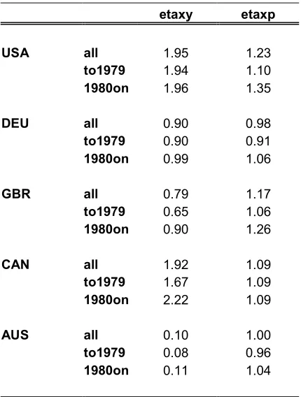
the elasticities of each components. Table 1shows the net tax elasticities to
output and to the GDP deflator in each country over the whole sample and
the main subsamples.27 The output elasticity is very low in Australia, mainly
for two reasons: the quarterly output elasticity of direct taxes on individuals is zero, because both the estimated output elasticity of real wages to employ-ment and of employemploy-ment to output are zero; and corporate income taxes have zero contemporaneous elasticity to their tax base, because quarterly install-ments are paid on the previous year’s assessed tax liability. The elasticity is slightly larger in the UK, which has a similar tax system to Australia but a small positive output elasticity of employment; it is still larger in West
Ger-many, with a still higher output elasticity of employment.28 It is highest in
Canada and USA, the only two countries where corporate income taxes have
a positive contemporaneous elasticity to corporate profits (see Appendix1).
It is well known that in quarterly data corporate profits are highly elastic to
output (in both Canada and the US, the estimated contemporaneous output
elasticity of profits is above 4): this accounts for the large contribution of
corporate income taxes to the aggregate elasticity of net taxes in countries with a non-zero contemporaneous elasticity of corporate income tax revenues
26One could argue that the individual income tax base includes interest income, which
would imply a positive interest rate semi-elasticity of individual income taxes. Yet it also includes dividend income, which might covary negatively with the interest rate. Like for the effects of prices, the effects of interest rates on corporate income tax revenues are extremely complex. Canzoneri et al. [2002] conduct a careful exercise to quantify the interest semi-elasticity of net taxes.
27Note that in general this elasticity varies over time, because so do the real wage
elasticity of tax revenues per person computed by the OECD, the estimated elasticities of real wages to employment and of employment to output, and the estimated output elasticities of corporate profits.
28Note that in all these three countries, the estimated employment elasticity of real
wages is either negative (Australia, West Germany) or positive but with a t-statistics below1(UK), hence it has been set to 0 according to the rule described above.
to corporate profits.
4
A
fi
rst look at the estimates
4.1
Do the
fi
scal shocks make sense?
Are the estimated fiscal shocks reasonable? This is a rather loose question,
but a legitimate one (see Rudebusch [1998]). Since the key facts of US fi
s-cal policy are much better known, I will limit the analysis to the US case.
Figure1 displays the estimated government spending and net tax shocks,egt
andet
t,from the benchmark 5 variable VAR on the whole sample, multiplied
by the average share of government spending and net taxes in GDP, respec-tively, to express them as shares of GDP. The shaded areas correspond to the three years following and including the onset of the two Ramey and Shapiro
episodes in this sample, the Vietnam war buildup that started in 1965:1and
the Carter- Reagan buildup that started in 1980:1.
The estimated shocks capture well thefirst buildup, much less so the
sec-ond one. There are several reasons for this: total government spending on
goods and services rose at a much faster rate in 1966 and 1967 (10 percent
and 7 percent, respectively) than in 1980 ,1981and1982 (2, -.1, and 1
per-cent, respectively). It is not often appreciated that, while defense spending
rose at an average rate of about 6% between 1980 and 1981, non defense
current spending on goods and services did not move in real terms, and
non-defense capital spendingfell at an average rate of about 4 percent. Note that
the estimated fiscal shock captures much better the increase in government
spending on goods and services between1984 and1987, when the latter rose
at an average rate above 4 percent, with non-defense current and capital government spending rising at average rates of 3 and 6 percent, respectively.
The structural net tax shock captures well the 1968 tax surcharge and
the (much larger) 1975. It is mostly positive between 1980 and 1982; this
however is easily explained in view of the large fall in GDP per capita in
1980 (-1.3 percent) and especially in1982 (-3 percent).
4.2
Subsample stability
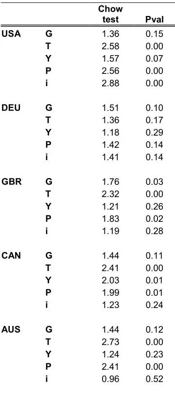
Table 2 displays the results from a standard Chow test on each reduced form
regression, with a break point in 1980:1 (1975:1 in West Germany). There
is substantial evidence of instability: in each country except West Germany
at least two of the five Chow tests have a p-value smaller than .05. We will
in the two subsamples. 29
5
The e
ff
ects of government spending on
out-put
5.1
E
ff
ects on aggregate GDP
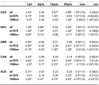
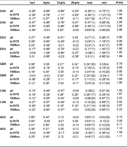
Table 3 and Figure 2 display the effects of a shock toegt equal to1percentage
point of GDP30, from a VAR in 5 variables with g and t ordered first and
second, respectively; the benchmark case displayed in this table also assumes an elasticity of real government spending to prices equal to -.5. To allow a comparison of the results across the 5 countries in a compact way, the table
displays the responses of GDP on impact and after 4, 12 and 20 quarters,
and the maximum and minimum GDP response up to 20 quarters, with the quarter at which it occurs (the maximum GDP response will also be called the “government spending multiplier” in what follows). The two lines on each side of the impulse response give one standard error bands, computed by Monte Carlo simulations based on 500 replications, as in e.g. Stock and
Watson [2001].
Over the whole sample, the impact response is positive and significant
in all countries. For the US, this is consistent with the positive response estimated by Blanchard and Perotti [2002], Edelberg, Eichenbaum and Fisher
[1999], Fatas and Mihov [2001], Canzoneri, Cumby and Diba [2002], and
Mountford and Uhlig [2002]. The size of the impact response is similar in all countries, between .3 and .4 percentage points (pps) of GDP except in West
29Even if the break were in a part of the structural VAR different from thefiscal policy
equations, it would appear in the whole reduced form and hence it would confound the identification of thefiscal shocks and the impulse responses to fiscal shocks.
The Chow test assumes that we know the time of the possible structural break, which we do not. There is mounting evidence in some recent literature of a breakdown in several macroeconomic relations around 1980 (see e.g. Stock and Watson [2002]). A downside of this procedure is that the break date chosen here is not strictly speaking exogenous, implying that the critical values of the conventional Chow test used here are too small.
A common alternative would have been to use a test, like the Andrews [1993] sup-Wald test, that does not assume such knowledge. But because of the very large number of parameters in the reduced form, the small sample properties of the latter test might be problematic.
30The impulse response of government spending and taxes are multiplied by their
re-spective average shares in GDP to obtain impulse responses in terms of shares of GDP. The actual response of government spending on impact is usually slightly different from
1, because of the feedback from ouput and price changes togt(recall that the shock is on
egt).
Germany, where it is 1.30 pps of GDP. In fact, over the first 3 years, in all
countries the largest effect on GDP occurs on impact; in the US, after about
4 years GDP has the absolute peak at about 1 pp of GDP. Thus, in no case
is the maximum GDP response much larger than 1, and in three countries
it is less than .5.31
These results, however, hide a substantial difference between the first
and second halves of the sample. When the model is estimated over the
two subsamples separately32, the pattern that emerges is rather clear: in
all countries except Australia, the effects of government spending shocks on
GDP in the post-1980 period are substantially smaller than in the pre-1980
period. In fact, in the post-1980 sample the response of GDP in thefirst four
countries is never significantly positive (except for West Germany on impact),
and it becomes significantly negative within thefirst 3 years. The minimum
response in all these countries is always smaller than -1, and significant.
One may wonder whether these results are due to a fundamental difference
in the government spending process over the two subsamples, in particular if the government spending response to its own shock is less persistent in the
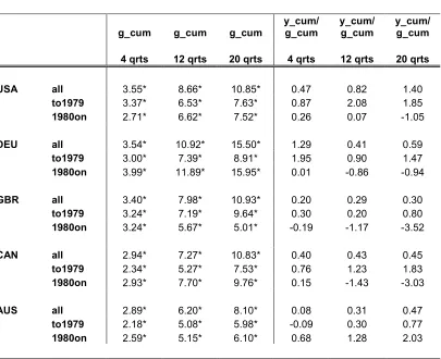
post-1980 period. Table 4 shows clearly that this is not the case. The
cumu-lative response of government spending (as a share of GDP) to a government
spending shock at quarters 4, 12 and 20 (columns 1to 3) is remarkably
sim-ilar across countries: for instance, at quarter 4 in the whole sample it ranges from 2.89 pp of GDP in Australia to 3.55 in the US. It is also similar across subperiods, with the exceptions of West Germany and the UK after 3 or more years.
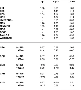
The cumulative multipliers33 (columns 4 to 6 of Table 4) provide an even
clearer picture: except for Australia, they are uniformly much higher in the
pre-1980 period than in the post-1980 period. In the latter, the
cumula-tive output multiplier is 0 after 4 quarters, and substantially negacumula-tive after
12 quarters (except in the US where it is essentially 0). As before, these
inequalities are reversed in Australia.
Note that the largest multiplier at 4 quarters is observed in West
Ger-31The shape of the impulse response is qualitatively similar in all countries (see Figure 2): after the initial rise, GDP starts declining, and after about 4 quarters it rises again; only in Germany and the US, however, is this second increase economically and statistically significant.
32When estimating the model over different subsamples, each time I recompute the
average elasticities over the relevant subsample. In doing so, if data are available I also reestimate the output elasticity of employment and the employment elasticity of wages over the relevant subsamples.
33The cumulative multiplier at quarter x is defined as the ratio of the cumulative
many, at 12 quarters in the US, and at 20 quarters in the US and Canada. Hence, while the results are mildly supportive of the notion that the most closed economy of the group tends to have larger multipliers, the ranking is not as clear cut as a standard leakage argument would suggest.
It is interesting to compare the estimated cumulative multipliers from this exercise with the cumulative multipliers typically provided by large scale
econometric models. This is done in Table 5.34 The large scale
macro-econometric models tend to predict larger cumulative multipliers than those
estimated here, in particular those estimated on the post-1980 sample.
5.2
The role of monetary policy
One could argue that differences in the government spending multipliers,
both over time and across countries, might be caused by differences in the
behavior of the monetary authorities.
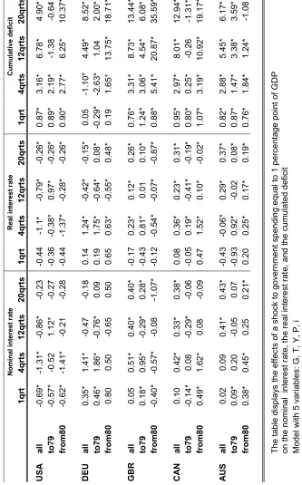
Table 6 displays the effects of a unit shock to governments spending on
the nominal (first 4 columns) and real (columns 5 to 8) short interest rates,
as well as on the cumulative deficit (last 4 columns).35 Consider the nominal
interest rate first. In the US, it falls on impact in all three samples; even
after 4 quarters, it declines by -.5 pps in the pre-1980 sample and by1.4 pps
in the post-1980 sample.
This response is puzzling, and indeed it has puzzled other researchers that have also found it in US data, like Mountford and Uhlig [2002] and Edelberg,
Eichenbaum and Fisher [1999];36 yet, once again, it is not necessarily typical.
Outside the US, in the whole sample the nominal interest rateincreasesin all
countries, except in West Germany after12 quarters. In the post-1980 period,
the nominal interest rate falls also in the UK; in West Germany, Canada and Australia it increases, although in the former it is rather imprecisely estimated.
The real short term interest rate follows a similar pattern.37 Over the
34The multipliers of the macro econometric models are from Sims [1988], who in turn
summarizes the results of the Brookings comparison project (see Bryant et al. [1988]). It should be noted that some models have changed since then, in particular more models have incorporated forward - looking behavior.
Also, it is well known that it is very difficult to compare the output of simulations across models, because it is very difficult to hold ”everything else” constant. The use of cumulative multipliers is intended to minimize this problem.
35Strictly speaking, this exercise is fully meaningful only underflexible exchange rates. 36Canzoneri, Cumby and Diba [2002] find a prolonged, though small, increase in the
federal funds rate after a spending shock.
37The real interest rate is defined here asi
t−(Ept+4−pt). If the alternative definition
it−4(Ept+1−pt)had been used, in some cases the real interest rate would have displayed
whole sample, after 4 quarters it falls in the US and, very marginally, in Australia; it increases in the other countries. In all cases, the response is
rather precisely estimated. In the post-1980 period, it falls the US and in
the UK, and it increases in the other three countries.
Can the difference in the output responsebetween the pre- and post-1980
samples be explained by a stronger interest rate response in the latter? No.38
Only in Canada does the real interest rate at 4 quarters increase more in
the post-1980 sample than in the pre-1980 sample; in all other countries, it
increases less, or falls more.
Can the difference in the output response across countries be explained
by a different behavior of the real interest rate? The answer is unclear. In
the post-1980 sample, the real interest rate falls after 4 quarters in the UK,
but the cumulative multiplier at the same horizon is also negative. If one excludes the UK, the two countries with the largest real interest rate response
at 4 quarters in the post-1980 sample, West Germany and Canada, also have
the lowest cumulative multiplier.
What about the reverse direction of causality, i.e. can the behavior of
the real interest rate be explained by the cumulative deficit? Not really.
The last 4 columns of Table 6 display the cumulative deficit response to the
government spending shock. Consider the post-1980 sample for brevity. The
country with the largest increase in the cumulative deficit after 4 quarters,
the UK, also has the second largest fall in the real interest rate; conversely,
the country with the second smallest increase in the deficit, West Germany,
also has the second largest increase in the real interest rate at the same horizon.
5.3
Other robustness checks
All the impulse responses presented so far were recomputed under the as-sumption that government spending is ordered second, after net taxes. The
differences were minimal: typically the point estimates of the impulse
re-sponses at all horizons change by only a few undredthos of a percentage point.
a very large fall in thefirst few quarters (in the order of 3 or 4 pps), due to the large and irregular behavior of the price response in the veryfirst quarter.
The post-1980 sample in the US includes two possibly very different monetary regimes: the Volcker experiment and the subsequent Volcker-Greenspan regime. The results are robust to the omission of the Volcker experiment,1979:4 to 1982:3.
38One important caveat: the short-term real interest rate might not be the most
The results are also robust to the exclusion of some years between 1973
and 197639, and to the exclusion of other specific years, motivated by
stan-dard periodizations in monetary policy (for instance, the 1979:4 - 1982:3
Volcker experiment in the post -1980 period in the US, or the1990:4 -1992:3
hard-ERM period in the United Kingdom).
Finally, I routinely estimate all impulse responses over the post -
Bret-ton Woods flexible exchange rate period. In the interest of space, I do not
present these estimates; in general, they appear to be intermediate between the responses of the two subsamples.
6
E
ff
ects on GDP components
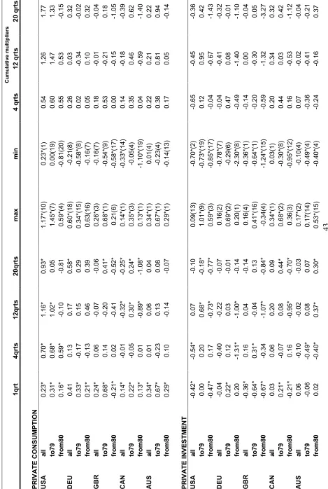
Table 7 displays the effects of government spending on GDP components.
The responses are derived from a 6 variable VAR, where each component of GDP is added in turn to the benchmark.
The behavior of private consumption largely mimics that of GDP: it
typi-cally increases on impact, and more so in the pre-1980 sample, although only
in Australia and the United Kingdom is the difference between the impulse
responses in the two samples substantial. In the pre-1980 sample, the
max-imum effect is larger than 1 in only one country, the US; in the post-1980
sample, it is never larger than .6. By quarter12, in the post-1980 quarter the
response is either insignificantly different from 0, or significantly negative.
Perhaps more informative is the cumulative consumption multiplier (the cumulative change in consumption divided by the cumulative change in
out-put). In the post-1980 sample, by quarter 4 it is no greater than .2 , except
in the US where it is .55; by quarter12 it has fallen further or it has remained
essentially at its quarter 4 level.40
Note that once again the US appears to be an outlier; over the whole sample its maximum consumption response is double that of the next highest maximum, and its cumulative consumption response is also by far the highest
at all horizons (except for West Germany at 12 quarters).
The private investment responses are typically more irregular, hence
sum-marizing their shapes is more difficult. However, in general the response of
investment is smaller than the response of consumption; and once again the
39The exact periods I exclude are 1974:1 - 1976:4 in the US, and 1973:1 - 1975:4 in
Australia, Canada, UK and West Germany. These years are chosen on teh basis of the size of the log change in the price level, real output, real net taxes, and real government spending.
40Note that the consumption response is much weaker in the post-1980 period also in
Australia, where the GDP response displayed the opposite pattern.
responses at all horizons, the maxima and minima, and the cumulative
mul-tipliers, tend to be algebraically smaller in the post-1980 period, with very
few exceptions (mostly in Australia).
In the pre-1980 sample the investment response after12 quarters is
posi-tive in the USA and about 0 in all other countries; in the post-1980 sample,
at the same horizon it is significantly negative in all countries (except
Aus-tralia), and remarkably similar — between -.7 and -.1 pp of GDP. In thefirst
sample, the minima are significantly negative in four countries, between
-.4 and -.8 pps of GDP; in the second sample, the minima are significantly
negative in all countries, and large — between -.4 and -2.3 of GDP.
The cumulative multipliers paint a similar picture. They are much smaller
in the second sample (with the exception of Australia at quarters12 and 20),
and negative after 12 quarters.41
It is difficult to detect a regular pattern in the response of exports and
imports. In general, the responses are surprisingly large, and there is some evidence of a systematic positive response of imports. The US is once again an exception to both statements.
7
How important is monetary policy for
fi
scal
policy? The Sims conjecture
There are two reasons why it might be important to include interest rate
and prices in a VAR withfiscal policy. In the Brookings comparison project
of Bryant [1988], typically small scale econometric models displayed larger
fiscal multipliers than large scale, rational expectation models that included
interest rate and prices (see Table 4). Sims [1988] conjectured that these
results could be explained by the presence offinancial variables, like interest
rates and prices, in the larger scale models; these jump variables embody
expectations of future changes in fiscal policy, and absorb some of the
esti-mated effects offiscal shocks. To test the Sims conjecture, I have estimated
a three variable VAR which excludes the interest rate and the GDP deflator.
In order not to clutter the exposition, I do not report the results, but
the pattern that emerges is clear. Both the impact effects and the maximum
effects of government spending on GDP are smaller in the smaller VAR, albeit
usually by very small margins, in both the whole sample and the pre-1980
sample. In the post-1980 sample, the same effects tend to be slightly larger in
the smaller VAR, although again by very small amounts, with the exception of the UK.
A second rationale for including the interest rate is that in its absence
fiscal shocks might pick up the effects of interest rate shocks if there is some
systematic contemporaneous relationship between monetary and fiscal
pol-icy.42 The same results mentioned above speak against this interpretation.
Another way to address this issue is to reverse the ordering of the
(cycli-cally adjusted)fiscal policy variables and the interest rate (see also Mountford
and Uhlig [2002] for a similar exercise). In all specifications so far, cyclically
adjusted taxes and government spending could not respond contemporane-ously to the interest rate. Suppose instead we assumed the opposite ordering. This is conceptually inconsistent with the assumption that, because of
de-cision lags, fiscal policymakers cannot make discretionary changes to fiscal
policy in response to contemporaneous innovations in the other variables. However, this ordering attributes as much as possible of the variation in gov-ernment spending innovations to interest rate innovations. If the systematic
response of monetary policy to fiscal policy is important, one would expect
the results to differ substantially now that fiscal shocks are forced to be
orthogonal to interest rate innovations. However, the results on the GDP multiplier (not reported to conserve space) are very similar. In this sense,
controlling for monetary policy is not important when estimating the effects
of fiscal policy on output — a result noted already by Mountford and Uhlig
[2002] for the US.
8
The e
ff
ects of government spending on prices
Just as the output elasticity of taxes is a crucial parameter in estimating
the effects of taxes on GDP, so is the price elasticity of government spending
crucial in estimating the effects of government spending on prices.43 To see
what is involved, consider a simplified version of the model
up =γug+ep (6)
ug =αup+ eg (7)
where all inessential variables and superscipts have been omitted. γ is the
effect of government spending on prices; αis the elasticity of real government
spending to the price level; ut and ug are the reduced form innovations in
42Strictly speaking, this argument is relevant in aflexible exchange rate regime only. 43See Blanchard and Watson [1986] for an early application of the methodology used
here.
net taxes and government spending, and et and ep are the corresponding
structural shocks; as usual, corr(eg, ep) = 0 by assumption. If not all of
government spending is indexed, α< 0. Suppose the researcher assumes an
elasticityαb different fromα. Hence, the researcher will estimatebeg =ep+ (α
- αb)up, and
cov(beg, up) =cov(eg, up) + (α−bα)var(up) (8)
and solving for var(up)andcov(eg, up)
cov(beg, up) = γ 1−αγ
·
1 + (α−αb)γ 1−αγ
¸
var(eg) + (α−αb)
(1−αγ)2var(e
p) (9)
Thus, if γ > 0 (government spending has a positive effect on prices) but
the researcher underestimates (in absolute value) the price elasticity of
gov-ernment spending, typically the estimated effect of government spending on
prices will be smaller than the true one. Note also that this bias increases with the variance of the price disturbance.
Indeed, previous VAR investigations on the effects of fiscal policy in the
US, like Fatas and Mihov [2001] and Mounford and Uhlig [2002], have
of-ten found a negative effect of government spending on prices or inflation.44
These results are based on orthogonalizations with real governments spend-ing ordered before prices, thus implicitly assumspend-ing a zero elasticity of real government spending to the price level.
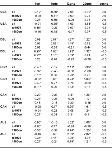
Table 8 displays the results of a shock to government spending on the price level under two alternative values for the price elasticity of the former:
0 (first three lines of each country) and -.5 (last three lines), from the same
specification used for Table 3. Table 8 makes three important points.
First, the price elasticity of government spending does matter in the short run: with few exceptions (and quantitatively minimal), the response at all horizons and in all samples is larger when the elasticity is -.5 than when it is 0. In a few countries, increasing the elasticity from 0 to -.5 changes the qualitative conclusions from this exercise quite dramatically: in Australia
in particular, the impact effect of a shock to government spending in the
pre-1980 sample changes from an implausible -1.6 percent to -.34 percent.45
44Canzoneri, Cumby and Diba [2002] alsofind a negative impact effect, followed by a
gradual increase. Edelberg, Eichenbaum and Fisher [1999]find a negative effect after an initial positive effect.
45For the reasons discussed above, even -.5 might be an underestimate of the true price
However, the price elastcity of government spending makes little difference
at quarter 12.
Second, for the response of the GDP deflator, even more than for the GDP
response, there is evidence of considerable subsample instability. Because the
effect on output is much more muted, one might expect to see a smaller effect
on the GDP deflator in the post-80 period. This is usually the case, except
in the UK:46 even with an elasticity of -.5, no country exhibits a significantly
positive price response at quarter 4 during this period. After 12 quarters,
only two countries exhibit a significantly positive response, the UK (1.13pps)
and Australia (.8 pps); in all the others, it is essentially 0.
Third, the US is, once again, an exception. It is the only country where
the response of the GDP deflator is negative after 4 and 12 quarters; notice,
however, that the large negative response over the whole sample estimated here and in other works becomes much smaller in the two separate
subsam-ples.47
The effects of a shock to government spending on the CPI deflator, instead
of the GDP deflator, are displayed in Table 9. The pattern that emerges is
very similar; except in Canada, in the post-1980 the CPI response appears a
bit stronger than the GDP deflator response, but the difference is substantial
only in West Germany.
The responses from a similar exercise, but based on a 6 variable VAR
which also includes a commodity price index, are also similar.48
9
The e
ff
ects of taxation
9.1
E
ff
ects on output
Table10 and Figure 3 display the effects of a shock to cyclically adjusted net
taxes equal to1percentage point of GDP. For each country, the table displays
the impulse responses under the benchmark output elasticity of net taxes
46Also, strictly speaking one would expect the opposite result in Australia, where GDP
increases more in the post-1980 sample.
47In fact, in all countries the response of the GDP deflator over the two subsamples is
considerably smaller, in absolute terms, than the response over the whole sample. In the UK, the response of the GDP deflator is explosive over the whole sample, while it appears stable over the two subsamples.
48Following much of the literature, the commodity price index is orderedfirst. Results
when it is ordered last (see Sims and Zha [1998]) are very similar. It should be noted that the reasons for controlling for a commodity price index when estimating the effects of fiscal policy on prices are much less compelling than when estimating the effects of a monetary policy shock.
(first three lines for each country), and under the same elasticity augmented by one (next three lines).
Considerfirst the results under the benchmark elasticity. The table makes
three points. First, the two countries with the largest output elasticity of
net taxes (see the last column), the US and Canada, are also the only
two countries where the impact effect of taxation on output is consistently
negative in all samples, although not larger than -.25 pps. In the other
countries, the estimated impact effect is always positive, and significant.
Second, there is again evidence of stronger negative effects of taxation
on GDP in the pre-1980 period than in the post-1980 one. For instance,
after 4 quarters the response of GDP is negative in all countries in the
pre-1980 period (although insignificant in Australia); in the post-1980 period it
is significantly negative in only two countries, Canada and the UK. More
generally, at the same horizon the output response is algebraically larger in
the second subsample in four countries out of five.
Third, the tax multipliers (defined as the minimum output response) are
not large: in the pre-1980 perios it is usually negative, but larger than one in
absolute value only in the US and in West Germany; in the post-1980 period,
it is between -.6 and -.7 in Canada and West Germany, close to 0 in the other countries.
The positive estimated output responses in Australia, UK and West Ger-many are suspicious. These are the three countries with the smaller output
elasticities of net taxes (in particular, in thefirst two the benchmark
elastic-ity is close to 0). As discussed, there are two reasons for this: the very small (or zero, in the case of Australia and the UK) estimated output elasticity of employment and employment elasticity of wages; and the zero elasticity of corporate income taxes to its base, due to the fact that corporations can pay quarterly installments on the basis of the previous year’s assessed tax
liabil-ity. This has a large effect on the estimated output elasticity of net taxes,
given the large weight of the corporate income tax in the net tax elasticity. Both conditions are implausible. In particular, it is likely that
corpora-tions would choose to pay quarterly installments based on expected profits,
if these differ greatly from the previous year’s profits. For each country, the
second set of rows in Table 10 displays the impulse response of output
un-der an assumed output elasticity of net taxes equal to the benchmark value,
augmented by 1. As expected, the response of output falls algebraically at
virtually all horizons. But in Australia and in the United Kingdom it often remains positive, or negative but stubbornly small. Reassuringly, note that the size of the tax multiplier seems to be largely independent of the net tax elasticity.