White Rose Research Online URL for this paper:
http://eprints.whiterose.ac.uk/144653/
Version: Accepted Version
Article:
Li, Y, Zhang, S, Zhang, J et al. (3 more authors) (2019) Data-driven Multi-objective
Optimization for Burden Surface in Blast Furnace with Feedback Compensation. IEEE
Transactions on Industrial Informatics. ISSN 1551-3203
https://doi.org/10.1109/TII.2019.2908989
(c) 2019, IEEE. This is an author produced version of a paper published in IEEE
Transactions on Industrial Informatics. Uploaded in accordance with the publisher's
self-archiving policy. Personal use of this material is permitted. Permission from IEEE must
be obtained for all other uses, in any current or future media, including
reprinting/republishing this material for advertising or promotional purposes, creating new
collective works, for resale or redistribution to servers or lists, or reuse of any copyrighted
component of this work in other works.
[email protected] https://eprints.whiterose.ac.uk/
Reuse
Items deposited in White Rose Research Online are protected by copyright, with all rights reserved unless indicated otherwise. They may be downloaded and/or printed for private study, or other acts as permitted by national copyright laws. The publisher or other rights holders may allow further reproduction and re-use of the full text version. This is indicated by the licence information on the White Rose Research Online record for the item.
Takedown
If you consider content in White Rose Research Online to be in breach of UK law, please notify us by
Data-driven Multi-objective Optimization for
Burden Surface in Blast Furnace with Feedback
Compensation
Yanjiao Li, Sen Zhang, Jie Zhang, Yixin Yin, Wendong Xiao,
Senior Member, IEEE,
and Zhiqiang Zhang
Abstract—In this paper, an intelligent data-driven optimization scheme is proposed for finding the proper burden surface distribution, which exerts large influences on keeping blast furnace running smoothly in energy-efficient state. In the pro-posed scheme, production indicators prediction models are firstly developed using kernel extreme learning machine algorithm. To heel, burden surface decision is presented as a multi-objective optimization problem for the first time and solved by a modified two-stage intelligent optimization strategy to generate the ini-tial setting values of burden surface. Furthermore, considering the existence of approximation error of the created prediction models, feedback compensation is implemented to enhance the reliability of the results, in which, an improved association rules mining method is developed to find the corrected values to compensate the initial setting values. Finally, we apply the proposed optimization scheme to determine the setting values of burden surface using actual data, and experimental results illustrate its effectiveness and feasibility.
Index Terms—Burden surface, blast furnace, multi-objective optimization problem, kernel extreme learning machine, feedback compensation.
I. INTRODUCTION
I
N the metallurgy industry, blast furnace (BF) represents an important process unit to produce the molten iron with high energy consumption [1], [2]. Thereinto, burden distribution scheme in the upper part of BF plays a crucial role in BF operation, which influences the gas flow distribution, and the utilization ratio of heat and chemical energy [3], [4]. Accordingly, the key to keep a smooth and stable operation environment is to form a proper burden surface, further it will achieve higher productivity, lower fuel rate and better quality of molten iron [5]. However, during the BF ironmak-ing process, many complicated chemical reactions and heat transport phenomena occur inside the furnace as the solid materials move downward and hot gases flow upward, so it is difficult to establish the mechanism model to accurately describe the effect of burden surface on the state of BF [6], [7]. In practice, the parameters corresponding to burden surface areThis work was supported in part by the National Natural Science Foundation of China under Grants 61673056, 61673055, 61673125, 61333002, the Beijing Natural Science Foundation under Grant 4182039 and the National Key Research and Development Program of China under Grant 2017YFB1401203. Y.J. Li, S. Zhang, J. Zhang, Y.X. Yin, and W.D. Xiao are with the
School of Automation & Engineering, University of Science and
Tech-nology Beijing, Beijing, China, 100083 (e-mails: [email protected], [email protected], [email protected], [email protected], [email protected]).
Z.Q. Zhang is with the School of Electronic and Electrical Engineering, University of Leeds, Leeds, U.K., LS2 9JT (e-mail: [email protected]).
usually tuned by experienced operators without optimal setting and system model as guidance. Such kind of manual tuning cannot make a fast and accurate adjustment of burden surface to ensure production indicators to be within the target ranges and track the dynamic production state well. Therefore, how to determine the optimal burden surface is still a challenging issue.
Most of the existed research works focus on thermal state prediction and burden distribution behaviors analysis for mon-itoring and controlling BF production process. For example, Li et al. [8] developed a fuzzy classifier for the development tendency of hot metal silicon content (HMSC). Jian et al. [9] proposed a novel binary coding SVM algorithm to judge the BF state. Liu et al. [10] demonstrated a concurrent monitoring method of the molten iron quality-relevant process faults, quality specific fault and process specific fault. Zhao et al. [11] established a comprehensive model from flow control gate to stock surface in detail and analyzed the non-uniformity phenomenon. Shi et al. [12] proposed a new stockline profile formation model and a stepped burden descending strategy to ensure the higher accuracy. The aforementioned investigations may assist operators to evaluate the production state and guide the charging process to achieve the desired burden surface. In terms of the optimal setting of burden surface, it is basically given by the operators based on their operational experience. To our best knowledge, researchers rarely attempted to de-termine the optimal setting of burden surface. Only Li et al. [13] adopted the self-optimizing method to establish the reasoning mechanism and constructed multiple sets of burden surface by K-means clustering algorithm, which obtains the local optimum and cannot ensure that the production indicators are within their target ranges.
profile [18]. Thus, inspired by the existed research works, the optimal setting of burden surface that satisfy the key production indicators can be obtained by employing data-driven based optimization techniques.
In this paper, an intelligent data-driven optimization scheme is proposed for achieving the optimal setting of burden surface using the collected data and it does not need to know the process dynamic model. It is worth noting that this is the first attempt to consider the burden surface decision as an optimization problem and solved based on data-driven tech-nique. The proposed scheme can adjust the burden surface setting values according to the variety of production state with three modules, i.e., kernel extreme learning machine (KELM)-based production indictors prediction model, a two-stage multi-objective optimization-based initial setting model, and an improved Apriori approach-based feedback compensation model. In addition, comprehensive experiments are performed using the actual production data to validate the effectiveness and feasibility of the proposed scheme.
The main contributions include the following aspects: 1) From a new point of view, optimization of burden surface in BF ironmaking process is addressed, to the best of our knowledge, it has not been considered before;
2) In order to avoid the lack of understanding on physical and chemical reactions inside BF, production indicators mod-els are created using KELM, which can avoid the non-optimal hidden node problem and ensure the stable performance;
3) The main target of BF ironmaking process is to obtain the smooth and stable operation environment and further achieve the energy-saving and consumption-reducing production with high-quality molten iron, in which involves multiple objec-tives (i.e., energy consumption indicator and production costs indicator). To ensure that ironmaking process can achieve satisfactory performance, the production indicators need to be maintained at the admissible ranges. In addition, these indicators are the two competing objectives which need to be taken into consideration. Therefore, the optimal setting of burden surface is considered as a multi-objective optimiza-tion problem (MOP), and the corresponding two-stage multi-objective optimization strategy is developed to find the initial setting values;
4) Due to model approximation error, an improved Apriori algorithm is implemented to discover the complex interrela-tions from the operating data to compensate the initial setting values of burden surface to enhance the reliability of results.
The remainder of this paper is organized as follows. Sec-tion 2 presents the problem descripSec-tions. The details of the proposed intelligent data-driven optimization scheme for de-termining the optimal setting values of burden surface are reported in Section 3. Section 4 reports the experiments and results using the actual data collected from a BF. Finally, the conclusions are given in Section 5.
II. PROBLEM DESCRIPTIONS
In this section, the present adjustment status of burden surface is firstly given. Then, the primary production objectives
Tuyere
Molten Iron Phased Array Radar
Burden Surface Ore & Coke
200ć Throat
Shaft
Bosh
Hearth1200ć 2000ć 1500ć 500ć
1000ć Descending
burden Ascending
gas
Preheated air, enriched oxygen Chute
Chute Cross Temperature Furnace Wall
Burden Surface
n n
Belly
[image:3.612.315.559.52.217.2]Burden Surface
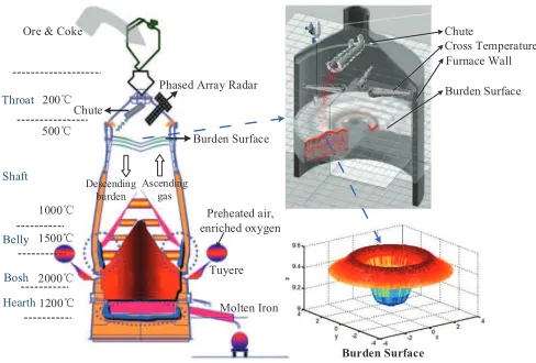
Fig. 1. Blast furnace ironmaking process and burden distribution
of BF ironmaking process are analyzed. Finally, the discretiza-tion of burden surface is described. These will motivate the problem formulation.
A. Actual adjustment status description of burden surface
As shown in Fig. 1, during the ironmaking process, the solid raw materials, including coke and ore, are fed into the top of furnace layer by layer with certain quantities, while the high-pressure preheated air and some auxiliary fuels are blown into the bottom through the tuyeres. A series of complicated chemical reactions and heat transport phenomena occur in the different zones under the different temperatures due to the downward movement of raw materials and the upward flow of hot gases. Finally, the molten pig iron flows to the furnace hearth at regular interval [19], [20], [21], [22], [23]. The radial distribution of the charged solid raw materials, i.e., burden surface (see the right of Fig. 1), influences the pressure loss and local mass flows of solid and gas inside the furnace and further affects the indirect reduction degree of the ore [24], [25].
As a matter of fact, the scheduling department personnel firstly determines the production indicators (denoted byP∗
k),
and the corresponding target ranges(Pkmin, Pkmax)according
to the production plan, where k denotes the number of the key production indicators, Pkmin and Pkmax are the lower
and upper bounds, respectively. Then, according to current production state, operators adjust the setting values of burden surface (denoted by bst = {bst,i}, where i represents the
constrains. Thus, it cannot guarantee the optimality of pro-duction indicators. Accordingly, it is necessary to develop an appropriate adjustment strategy of burden surface.
B. Primary production objectives of BF ironmaking process
In practice, gas utilization ratio (GUR), a conversion ratio of COtoCO2, is an important indicator to measure the operating
state and energy consumption [26]. If the burden surface profile is reasonable, the chemical reactions are sufficient, the gas utilization degree will be high. Hence, the improvement of GUR is the embodiment of technical progress in BF operation. Besides, coke ratio (CR) is another indicator we should consider, which indicates the amount of coke consumed by smelting one ton of qualified pig iron, so it is urgent to decrease CR for reducing the production cost.
Permeability index (PI) is a significant symbol to measure whether gas permeability inside the furnace is kept in its admissible range. When PI is within a specific range, a dy-namic balance between ascending gas and descending burden materials is achieved. If not, it indicates the gas permeability becomes worse, which may cause the charge material fall to be difficult. In severe cases, it will lead to hanging.
In addition, HMSC is a main parameter by which product quality of pig iron is measured [27]. In terms of energy, it is desirable to keep the BF ironmaking process at a low HMSC, while still avoiding the danger of cooling the hearth [6].
Accordingly, the production objectives of the optimization BF operation are specifically described as follows:
1) Aim to maximize GUR and minimize CR within their target ranges;
2) Take two aspects of requirement as constraints, including PI and HMSC, keeping them within prescribed bounds;
3) Keep the operation at its best by adjusting the setting values of burden surface.
C. Discretization of burden surface
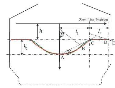
Burden surface is actually a continuous shape, because it is formed by the accumulation of raw materials. Thus, it needs to be discretized to implement the optimal setting. In general, charging regulation usually adopts platform plus funnel mode, the main concerns of the operators are the width of platform, the depth and width of funnel [28]. Fig. 2 illustrates the feature extraction for burden surface discretization. The green curve is the actual curve obtained by analyzing the data measured by radar. In accordance with operational cognition, seven features are extracted to represent the burden surface, including width of funnel l1, width of platform l2, distance between zero
position and burden surfaceh1, depth of funnelh2, inclination
angle of funnel α, central angle of funnel β and inclination angle of edge γ. The mathematical representations of the aforementioned seven features are as follows:
h1=|yC|, h2=|yA−yC|, l1=|xC−xA|,
l2=|xD−xC|, α= arctan (
yC−yA
xC−xA )
,
β= arcsin(xB−xA
R
)
, γ= arctan (
yE−yD
xE−xD )
. (1)
Zero Line Position
A
B
[image:4.612.338.527.49.193.2]C D E
Fig. 2. Schematic diagram of burden surface discretization
where (xi, yi) is the coordinates of point i and
R=(yB−yA)2+(xB−xA)2
2(yB−yA) .
In addition, in order to ensure the correctness of the sev-en features and the implemsev-entation of the multi-parameter optimization of burden surface, it is necessary to establish the regression model of burden surface feature parameters. “Curve-Line-Line-Curve” mode is used to fit the burden surface profile. The coordinate values of the key points A, B, C, D, E need to be determined firstly. The relationship between the coordinate values of these five points and the burden surface feature parameters are as follows:
RA: (0, h1+h2)
RB: (R·sinβ, h1+h2+R−R·cosβ)
RC: (l1, h1)
RD: (l1+l2, h1)
RE: (r, h1+ (r−l1−l2)·tanγ)
(2)
Then the regression model can be represented as:
y=
h1+h2−R+ √
R2−x2,0≤x < Rsinβ
yC−yB
xC−xB(x−xB) +yB, Rsinα≤x < l1 h1, l1≤x < l1+l2
(x−xD)tanγ+yD, l1+l2≤x < r
(3)
The red curve denotes burden surface obtained by the extracted features in Fig. 2. We can find that the red curve is in good agreement with the green curve, which indicates that the extracted features can well characterize the burden surface. Therefore, seven feature parameters of burden surface can be used as decision variables.
Overall, burden surface setting can only be adjusted by experienced operators, which cannot guarantee the optimality of production indicators. Inspired by the practical data-driven techniques, considering the characteristics and production tar-gets of BF ironmaking process, the problem that needs to be solved is how to determine the setting values of burden surface (i.e., burden surface features) with a large number of data collected from BF to provide better decision support.
III. PROPOSED SCHEME FOR BURDEN SURFACE OPTIMIZATION
Multi-objective Optimization
Burden distribution matrix control
mechanism
Charging device
Burden surface measurement
Production state analysis Constraints Initial setting
values g Feedback Compensation Strategy
Prediction Model of Production Indicators
+ _
Burden Surface Parameters Operating Status Parameters
+ _ +
[image:5.612.51.303.54.165.2]tting s
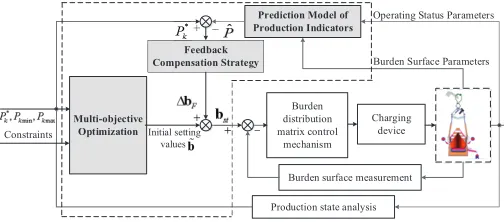
Fig. 3. Scheme of burden surface optimization for BF ironmaking process
A. Overall framework of the proposed scheme
The intelligent data-driven optimization scheme for deter-mining the setting values of burden surface is illustrated in Fig. 3. The proposed scheme has three modules, including production indictors modeling, multi-objective optimization s-trategy for burden surface and feedback compensation. Firstly, the optimization problem requires the model of production indicators for performing the optimization. Due to the high complexity of the furnace interior and its nonlinear nature, the model of the ironmaking process is difficult to be estab-lished in practice. KELM, which has fast learning speed and good generalization performance without random projection mechanism, is employed to create the production indicators model.
After that, according to the production purpose of high efficiency and low consumption, the optimal setting of burden surface is summarized as a MOP. Then, the corresponding mathematical description is given. In addition, in order to obtain more comprehensive Pareto optimal solutions, a mod-ified two-stage intelligent strategy optimization algorithm is proposed to solve the MOP and generate the initial setting values of burden surface.
Finally, if the models of production indicators are accurate, the initial setting values of burden surface obtained in the aforementioned step can ensure that the production indicators remain with their target ranges. However, due to the existence of model approximation error, this may not be ensured. There-fore, a feedback compensation strategy is presented, in which an improved association rule mining method is used to find the corrected values to compensate the initial setting values of burden surface using the difference between predicted values of production indicators and their target values.
All notations used in describing the proposed data-driven optimization scheme for determining the setting values of burden surface are presented in Table I.
B. Modeling of production indicators
With the ironmaking mechanism analysis, burden surface profile and operating state parameters affect the production indicators. Thus, production indicators can be described as
(P1, P2, P3, P4) =f(b,ψ) (4)
wheref(·)is an unknown nonlinear function, P1, P2, P3, P4
indicate GUR, CR, PI and HMSC, respectively, b =
{bi, i= 1,2, . . . ,7} = {l1, l2, h1, h2, α, β, γ} is the burden
surface features, andψ is the operating state parameters. Denote τ = (b,ψ) and o = (P1, P2, P3, P4). The model
f(b,ψ) = f(τ) can be approximated by the ELM model
ˆ
fELM(τ,ν):
ˆ
fELM(τ,ν) =h(τ)ν (5)
whereh(τ)is the hidden layer output matrix,νis the output
weight vector between the hidden layer and the output layer.
h(τ)can be randomly assigned before training and does not
require manual intervention [29], [30], [31], which is a salient feature as compared to other data-based modeling approaches (e.g., BP and SVM). Thus, onlyν needs to be identified.
For a given sample setℵ={τi,oi|i= 1,2, . . . , N}, where
N is the number of samples, τi = [τi1, τi2, . . . , τid] is a d
-dimensional input attributes, and its respective output variables
oi = [oi1, oi2, . . . , oim] is a m-dimensional vector, and here
m= 4. The following optimization problem is formulated to identify ν:
min :J =1 2∥ν∥
2
+C 2
N
∑
i=1 ξ2i
s.t.,h(τi)ν=oi−ξ
i
(6)
where C is the regularization parameter, ξi is the training error.
According to the Karush-Kuhn-Tucker condition, it can be solved by the following dual optimization:
L(ν,ξ,ω) = 1 2∥ν∥
2
+1 2∥ξ∥
2
−ω(h(τ)ν−o+ξ) (7)
whereω= [ω1, ω2, . . . , ωN]is the Lagrange multiplier
corre-sponding to the training samples. Then, νcan be obtained:
ν=HT
(I
C +H
TH
)−1
o (8)
Such that the ELM model fˆELM(τ,ν)in Eq.(5) becomes
ˆ
fELM(τ,ν) =h(τ)HT
(I
C +H
TH
)−1
o (9)
Then, a kernel matrixΩof ELM is defined by Huang et al.
[32], which can be written as
ΩELM =HHT :ΩELM i,j=K(τi,τj) (10)
Finally, replacing HHT in Eq.(9) with ΩELM from
Eq.(10), the KELM model can be obtained as
ˆ
fKELM(τ,ν) =h(τ)HT
(I
C +ΩELM )−1
o (11)
Remark 1: The significant benefits of KELM are that it
TABLE I
NOMENCLATURE USED IN THE INTELLIGENT DATA-DRIVEN OPTIMIZATION SCHEME FOR DETERMINING THE SETTING VALUES OF BURDEN SURFACE
Notation Description
Pk,Pk∗,Pkmin,Pkmax,Pˆk Actual valuetarget value, minimum value, maximum value and prediction value of thekth production indicator
∆Pk Error between the target values and the predicted values of production indicators
bst,∆bF,˜b Optimal setting values, corrected values, initial setting values of burden surface
b={h1, h2, l1, l2, α, β, γ} Seven burden surface features
r Radius of BF
ψ Operating state parameters
ν Output weight vector between the hidden layer and output layer in ELM
h(τ) =h(b,ψ) Hidden layer output matrix
N The number of samples
ℵ={τi,oi|i= 1,2, . . . , N} Sample set
C,ξi Regularization parameter and training error in ELM model
ω= [ω1, ω2, . . . , ωN] Lagrange multiplier
Ω Kernel matrix
Φ,Ψ Pareto optimal solution sets obtained by NSGA-II and MOPSO
ℜ Evaluation matrix of TOPSIS method
I(b, P) Mutual information function
µ(·) Probabilistic density function of variable(·)
A,C,D Condition attribute set, decision attribute set and data table in association rule mining
∇(·) The value of variable(·)
min sup, min conf Minimum support threshold and the minimum confidence threshold
Lk Frequentk-itemsets
σ Kernel bandwidth of Gaussian kernel function
C. Determing the initial setting values based on multi-objective optimization
As mentioned in the Section II-B, burden surface optimiza-tion is actually a MOP. Given the target values and ranges for Pk, determine the burden surface features such that
J ∼ {maxP1,minP2} (12)
subject to the constrains:
Pkmin≤Pk ≤Pkmax, k = 1,2,3,4
bimin≤bi ≤bimax, i= 1,2, . . . ,7
(P1, P2, P3, P4) =f(b,ψ)
(13)
wherebimin andbimax are the lower and upper bounds ofbi.
In the constraints of Eq.(13), the first inequality guarantees the production indicators in target ranges, in which, the constraint on PI is to ensure the smooth and stable production, and the constraint on HMSC is to ensure the production of qualified hot metal.
It should note that the aforementioned optimization problem belongs to a nonlinear MOP with constraints. The most popular multi-objective algorithm based on meta-heuristic approach, known as multi-objective evolutionary algorithm (MOEAs), are considered the effectiveness in solving the MOP by providing a Pareto optimal solution set. Among the MOEAs, the non-dominated sorting genetic algorithm version II (NSGA-II) [33] is one of the most famous and successful ap-proaches with elitist strategy and diversity preservation mech-anisms. The salient features of NSGA-II are computationally efficient and less dependent on the sharing parameters. It has been criticized that it is easy to produce duplicate individuals.
In recent years, with the further research of MOEAs, new mechanisms and strategies have been developed to solve the MOP. For example, multi-objective particle swarm optimiza-tion (MOPSO) [34] was presented by Coello et al., which preforms better in solving the MOP. The merit of MOPSO has efficiency and fast convergence with external repository strategy and mutation operator. However, it is difficult to deal with some multi-frontal problems. They use different search strategies for exploring the feasible solution space and adopt different methods to handle constraints and selection mechanisms. In order to obtain more comprehensive Pareto optimal solutions, we take advantage of both the NSGA-II and MOPSO algorithms.
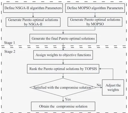
A two-stage intelligent decision process, as shown in Fig. 4, is implemented to determine initial setting values of burden surface. Specifically, in the first stage, in order to make full use of the advantages of different algorithms to get more comprehensive Pareto optimal solutions, NSGA-II and MOP-SO algorithms are firstly adopted to solve the optimization problem shown in Eqs.(12) and (13). All solutions obtained by the two algorithms are merged to find the final Pareto optimal solutions. However, even though the results are informative, the number of solutions may still be prohibitive for decision-maker. At this point, in the second stage, a ranking method called TOPSIS [35] is employed to rank the Pareto optimal solutions by the preference of operators to select a compromise solution.
Define NSGA-II algorithm Parameters Define MOPSO algorithm Parameters
Generate Pareto optimal solutions by NSGA-II
Generate Pareto optimal solutions by MOPSO
Generate the final Pareto optimal solutions
Rank the Pareto optimal solutions by TOPSIS
Satisfied with the compromise solution?
Obtain the compromise solution
Adjust the weights Assign weights to objective functions
Yes
No Stage 1
[image:7.612.63.286.51.247.2]Stage 2
Fig. 4. A two-stage intelligent decision process for determining initial setting values of burden surface
criteria,ℜ, is created to perform the computation of TOPSIS:
ℜ=
ϖ11
ϖ21
.. . ϖp1
ϖ12
ϖ22
.. . ϖp2
(14)
whereϖij represents the evaluation matrixR of alternative
i under evaluation criterion j. Finally, according to the oper-ators’ preference, their most satisfactory compromise solution (i.e., the initial setting values of burden surface b˜={˜bi, i=
1,2, . . . ,7}) can be found.
D. Improved Apriori algorithm based feedback compensation
Due to the existence of model approximation error, the ob-tained initial setting values may not guarantee the production indicators to be within their target ranges. In practice, the useful and valuable association relationship hidden in collected data needs to be mined and expressed by understandable sen-tences, which is of great significance for production decision-making. Therefore, motivated by the thought of control theory, a feedback compensation strategy is presented, which uses the association rules extracted from the large amount of data to find the corrected values to further compensate the initial setting values. In the proposed strategy, mutual information (MI) [36] method is used to select the burden surface features that need to be corrected, and the Apriori method as a powerful rules mining tool is used to discover the association rules (i.e., incremental rules relation between production indicators and burden surface features) from the collected data. Un-like general data mining, the essential relationship between variables is clear and the quantitative relationship between them needs to be mined in the industrial process data mining. Because the traditional Apriori method does not contain any prior knowledge about BF production, hence, considering the characteristics of BF production data, an improved Apriori association rule mining method is implemented to find the
feedback association rules. The proposed feedback compensa-tion strategy is a data-driven approach, which does not require process models.
1) Data-based compensation strategy: The initial setting
values are fed into the approximated nonlinear function in Eq.(4) to obtain the predicted values of production indicators
ˆ
Pk(k = 1,2). Define the error between the target values of
production indicatorsP∗
k and the predicted valuesPˆk as
∆Pk=Pk∗−Pˆk(k= 1,2) (15)
A lower bound ∆Pkmin is determined in advance by the
experienced operators. If |∆Pk|is greater that ∆Pkmin, it is
considered that the initial setting values need to be corrected. The corrected values are found by association rules method, which will be described in the next section. During the mining process, data preparation is firstly implemented to form data table. Because the burden surface features have different effects on production indicators, the features that closely related to production indicators are considered to be compensated. MI method is employed to analyze the influence degree of burden surface features on production indicators, and the burden surface features that need to be corrected can be selected based on the threshold of correlation coefficients. The MI is defined as
I(b, P) =
∫ ∫
µ(b, P) log µ(b, P)
µ(b)µ(P)dbdP (16)
where µ(·) represents the probabilistic density function of variable(·). The greater MII(b, P), the stronger the influence degree is.I(Pk, bi) (k= 1,2;i= 1,2,· · · ,7)is defined as the
influence degree of theith burden surface feature with respect to the kth production indicator. Then the influence degree of the ith burden surface feature with respect to the production indicators can be calculated by
I(bi) =
2
∑
k=1
I(Pk, bi) (17)
Thus, the selected burden surface features that need to be correctedbF ={bf, f = 1,2, . . . , F}are obtained.
Here A = {Pk,∆Pk,bF} denotes the antecedent of data
table (i.e., conditional attribute set) and is marked asclass1, and C = {∆bF} is called the consequent (i.e., decision
attribute set) and is marked asclass2, where∆bF ={∆bf}is
the corrected values of selected burden surface features. Thus, the data tableDcan be represented as
D={Pk,∆Pk,bF,∆bF} (18)
Then, the association rules form for feedback tuning via the proposed association rules method is expressed as
If Pk=∇(Pk)∧∆Pk=∇(∆Pk)∧bf=∇(bf) then ∆bf=∇(∆bf)
(19)
where∇(·) is the value of variable(·). After that, the final decision values of burden surface are written specifically as
bst,i=
{ ˜
bi, |∆Pk|<∆Pkmin
˜
bi+ ∆bf,|∆Pk| ≥∆Pkmin
2) Improved Apriori algorithm: Because there is no prior knowledge of BF production, the rules mined by the classical Apriori algorithm may not be correct. For this reason, an improved Apriori algorithm is implemented to discover more effective association rules whose detailed steps are as follows: Input: Database ℘ = D, minimum support threshold min supand minimum confidence thresholdmin conf.
Output: Feedback compensation association rules.
Step 1 (Discretization): Let r, r ∈ D, be a continuous variable and its range is ℓr = [ηrmin, ηmaxr ]. Discretization is
to divide the range of variable into finite interval of assigned symbols to generate⟨varaible, interval⟩pairs. Each variable is firstly encoded according to the order in database. Further, ℓr is divided intokr intervals, which is represented as
{
ℓr= [υ0r, υr1)∪[υr1, υr2)∪ · · · ∪ [
υrkr, υ r kr+1
]
ηmin=υr0< υ1r< υr2<· · ·< υkrr < υrkr+1=ηmax
(21)
where υr
i is the segmentation point of ℓr. The interval
length can be expressed as ρ = (ηrmax−ηminr )/k
r, thus the
segmentation points areηr
min+iρ, i= 1,2, . . . , kr. Meanwhile,
kr intervals are also coded as1,2, . . . , kr, respectively. Thus,
the database is discretized to convert into Boolean data form. Step 2 (Find the frequent 1-itemsetsL1): Scan the database
and calculate the support of each attribute. If it is greater than min sup, the frequent 1-itemsetsL1is found.
Step 3 (Find the frequent 2-itemsets L2): Let itemk and
iteml be any two attributes in the database. If frequent
itemsets only contain the conditional attributes or the decision attributes, then the invalid rules are generated. Thus, in order to avoid the two attributes from the same class, the selection requirement is given by
If class(itemk)̸=class(iteml) join itemk and iteml
inset (itemk, iteml) in frequent itemsets end
(22)
Step 4 (Find the frequentk-itemsetsLk): Find the next level
frequent itemsets untilLk =∅.
Step 5 (Generate the association rules): In order to mine the rules shown in Eq.(19), the following constraint is added:
If (class(itemk) =class1 & class(iteml) =class2) confidence =supp(itemk∪iteml)
supp(itemk) If confidence≥min conf
output: itemk→iteml end
end
(23)
IV. EXPERIMENT STUDIES USING ACTUAL DATA
In this section, comprehensive experiments are carried out using the actual industrial data to verify the effectiveness and feasibility of the proposed intelligent data-driven opti-mization scheme. In the following experiments, the data are collected from a medium-size BF with an inner volume of about 2500m3. In addition, some daily production data from
historical database are selected for analysis.
A. Production indicators modeling experiments
Some important and measurable variables influencing the production indicators are considered as the operating state parameters ψ, including blast volume (m3/min), blast tem-perature (◦C), blast pressure (kP a), top temperature(including
four-point temperature) (◦C), top pressure (kP a), differential
pressure (kP a), cross temperature (including center and edge) (◦C), oxygen enrichment (%). The corresponding burden
sur-face features are obtained after processing the acquired radar data (see Eq.(1)). For production indicators modeling, the indices are achieved through the average. In terms of HMSC prediction model, the sampling interval HSMC is one hour, and that of other indices are one minute, all variables are achieved through the 1-hour average of 1-minute variables. In addition, the raw data collected from the real system may contain some outliers, which may affect the performance of modeling and decision-making. These may be due to irregular behaviors of furnace interior in a certain period of time, furnace shutdown or some wrong readings. The elimination of outliers is performed to ensure the reliability. Furthermore, there is great difference in the magnitude of the variables. Considering the impacts of convergence and complexity on modeling, all samples are normalized into [0,1]to eliminate the influence of magnitude before applying in the experiments. We randomly select 1000 data pairs, the first 800 group-s are ugroup-sed for training the KELM modelgroup-s and othergroup-s for validating the created models. The Gaussian kernel function, i.e.,K(τi,τj) = exp
(
−σ∥τi−τj∥2
)
, is adopted in KELM, where σ is kernel bandwidth. There are two user specified parameters in KELM, i.e.,Candσ, which need to be selected appropriately to achieve good generalization performance. In this paper, both C and σ are searched from the range (
2−24,2−23, . . . ,225), whose optimal combination is chosen
as the one with the minimum testing error. For simplicity, we mainly discuss the procedure of selecting the optimal combination of(C, σ)in the data-based model of GUR. Fig. 5 details the effects of combination of (C, σ) on the model performance. Accordingly, the performance (i.e., testing error) is sensitive to the combination of (C, σ). There is a sharp decrease when C and σ are in the range of (
2−15,25) and (
2−25,225)
respectively. Then, with the increase of C, the testing error tends to be stable. The minimum testing error is achieved in a narrow range of such combination. Thus, the optimal combination can be chosen in this range, soC andσ are set as215 and2−15, respectively. For the models of CR,
PI and HSMC, the same procedures are preformed to select the corresponding optimal ones.
2^(−25) 2^(−15)
2^(−5) 2^(5)
2^(15)
2^(25) 2^(−25) 2^(−15)
2^(−5) 2^(5)
2^(15) 2^(25) 0.03
0.05 0.07 0.09 0.11
σ
C
[image:9.612.322.553.52.462.2]Testing error
Fig. 5. Effects of combination of(C, σ)on the model performance
TABLE II
RMSE, MAPEANDCCOFKELMFOR FOUR MODELS
Model RMSE MAPE CC
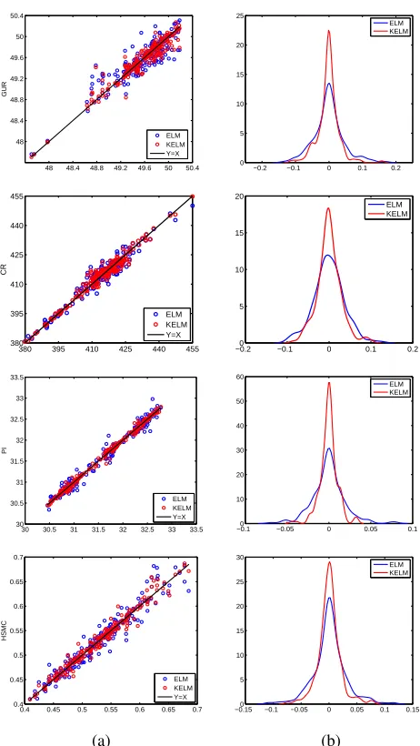
GUR 0.0310 0.0254 0.9581
CR 0.0284 0.0443 0.9845
PI 0.0124 0.0219 0.9971
HMSC 0.0211 0.0393 0.9758
PDF of predicted error of a good model should be a Gaussian distribution with smaller mean and variance, the PDF curves of predicted error are presented in Fig. 6(b). From Fig. 6(b), the error mean is 0 and the curve has only one peak, which are the Gaussian curve characteristic. Meanwhile, KELM gets a PDF with a higher and narrower shape, which shows that the errors are more concentrated near the mean (i.e., 0) and variance is less. Therefore, KELM can provide more accurate predicted results. Furthermore, the root mean squared error (RMSE), mean absolute percentage error (MAPE) and correlation co-efficient (CC) between actual values and predicted values of KELM are listed in Table II. As observed from Fig. 6 and Table II, KELM shows satisfactory performance for the four models, which can be used to provide the basis for subsequent optimization.
B. Determination experiments for the setting values of burden surface
1) Generation of initial setting values: For the MOP
for-mulated as Eqs.(12) and (13), the two-stage intelligent opti-mization strategy is used to determine the initial setting values
˜
b. The related variables used in the NSGA-II algorithm are:
population size is set toNpop= 200, the crossover probability
is assumed to be 0.95 and the mutation probability is set as 0.1. Similarly, for MOPSO, the swarm size is set as 200. In particular, the maximum iterations Itmax is very important
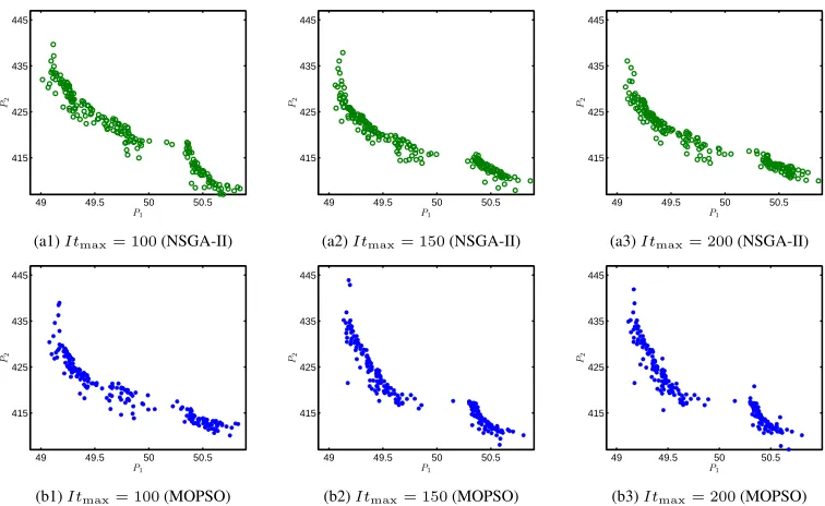
for the convergence of both algorithms. The Pareto optimal solutions obtained by NSGA-II and MOPSO algorithms with different maximum iterations are given in Fig. 7. From Fig. 7, with the increase of the maximum iterations, the solutions trend to stable gradually. Therefore, Itmax is seleted as 150
in both algorithms. The Pareto optimal solutions for each algorithm on a single production state are plotted in Fig. 8.
48 48.4 48.8 49.2 49.6 50 50.4 48
48.4 48.8 49.2 49.6 50 50.4
GUR
−0.2 −0.1 0 0.1 0.2 0
5 10 15 20 25
ELM KELM
ELM KELM Y=X
380 395 410 425 440 455
380 395 410 425 440 455
CR
−0.20 −0.1 0 0.1 0.2
5 10 15 20
ELM KELM
ELM KELM Y=X
30 30.5 31 31.5 32 32.5 33 33.5 30
30.5 31 31.5 32 32.5 33 33.5
PI
−0.10 −0.05 0 0.05 0.1 10
20 30 40 50 60
ELM KELM Y=X
ELM KELM
0.4 0.45 0.5 0.55 0.6 0.65 0.7 0.4
0.45 0.5 0.55 0.6 0.65 0.7
HSMC
−0.150 −0.1 −0.05 0 0.05 0.1 0.15 5
10 15 20 25 30
ELM KELM Y=X
ELM KELM
(a) (b)
Fig. 6. Scatter diagram of four production indicators models and PDF curve
of modeling error
The green circles and blue asterisks represent the NSGA-II solutions and MOPSO solutions, respectively. As can be observed, the solutions generated by both algorithms make the values of objective functions roughly in the same ranges and NSGA-II generates more solutions at the edge of the feasible solutions. In this sense, more comprehensive Pareto optimal solutions are obtained for operators to make decisions for meeting the actual production. From this figure, when GUR is above about 50.5, CR will not be decreased although GUR is increased. This phenomenon means that only focusing on improving GUR cannot ensure CR continue to decrease, which illustrates that GUR and CR are interrelated and conflicting and further clarifies that it is reasonable to summarize the burden surface optimization as a MOP.
[image:9.612.60.293.66.199.2]49 49.5 50 50.5 415
425 435 445
P1
P2
(a1)Itmax= 100(NSGA-II)
49 49.5 50 50.5
415 425 435 445
P1
P2
(a2)Itmax= 150(NSGA-II)
49 49.5 50 50.5
415 425 435 445
P1
P2
(a3)Itmax= 200(NSGA-II)
49 49.5 50 50.5
415 425 435 445
P1
P2
(b1)Itmax= 100(MOPSO)
49 49.5 50 50.5
415 425 435 445
P1
P2
(b2)Itmax= 150(MOPSO)
49 49.5 50 50.5
415 425 435 445
P1
P2
[image:10.612.113.491.56.288.2](b3)Itmax= 200(MOPSO)
Fig. 7. Pareto optimal solutions obtained by NSGA-II and MOPSO algorithms with different maximum iterations
49 49.5 50 50.5 415
425 435 445
P1
P2
[image:10.612.91.251.328.449.2]NSGA−II solutions MOPSO solutions
Fig. 8. Merged NSGA-II and MOPSO Pareto optimal solutions
found from Table III that these solutions provide useful infor-mation for operators to adjust the burden surface to cope with changes in production state. Actually, the selection of weight of each objective can be determined based on the production requirements at a certain time period and production state. If we pay more attention to cost, CR will be given a larger weight, on the contrary, GUR will be given a larger weight.
2) Generation of corrected values based on feedback
com-pensation strategy: The influence degree of each burden
sur-face feature on production indicators is calculated by Eqs.(16) and (17) and the results are demonstrated in Fig. 9. Based on these correlation coefficients, the burden surface features, l1, h2, α, β with the influence degree no less than 0.18 are
selected to be corrected. After that, the improved Apriori algorithm is applied to extract the useful rules, thus the corrected values are generated. For simplicity, only some of the rules are listed in Table IV.
3) Experimental results: The detailed analysis of
genera-tion of the initial values and the corrected values have been given in the above section. Then, the setting values can be achieved through Eq.(20). Based on the regression model of
TABLE III
TEN EFFICIENT SOLUTIONS WITHTOPSISSCORE
TOPSIS Decision Variables (burden surface features)
Score l1 l2 h1 h2 α β γ
0.7006 1.96 1.53 0.81 0.64 24.77 19.80 -7.01
0.9212 2.09 1.68 0.77 0.71 23.89 18.58 -6.83
0.8380 1.82 1.71 0.83 0.69 24.11 19.23 -6.62
0.9509 1.98 1.59 0.73 0.76 25.02 18.80 -6.53
0.9391 2.01 1.45 0.84 0.60 24.85 19.05 -6.70
0.8298 1.84 1.66 0.85 0.63 25.09 19.23 -6.92
0.7885 1.93 1.58 0.79 0.64 24.53 19.70 -6.77
0.9177 1.89 1.62 0.82 0.76 24.22 19.63 -6.73
0.8630 1.88 1.70 0.81 0.72 24.76 19.03 -6.81
0.9298 1.95 1.59 0.85 0.76 24.62 19.67 -6.79
l1 l2 h1 h2 α β γ
0.16 0.18 0.2 0.22
Burden surface features
C
o
rr
e
la
ti
o
n
co
e
ff
ici
e
n
[image:10.612.320.555.345.601.2]t
Fig. 9. Influence degree of each burden surface feature on production
indicators
feature parameters as calculated by Eq.(3), the shape of burden surface can be drawn and shown in Fig. 10.
TABLE IV
SOME OF THE ASSOCIATION RULES
No. Rules
Antecedent Consequent
1 P1(2) andP2(1) and ∆P1(2) and ∆P2(3) andb1(2) andb4(3) andb5(3) andb6(2) ∆b1(2)
2 P1(3) andP2(1) and ∆P1(2) and ∆P2(2) andb1(2) andb4(3) andb5(3) andb6(2) ∆b1(2)
3 P1(1) andP2(1) and ∆P1(2) and ∆P2(2) andb1(1) andb4(2)andb5(3) andb6(4) ∆b1(4)
4 P1(1) andP2(2) and ∆P1(4) and ∆P2(3) andb1(3) andb4(2)andb5(3) and b6(4) ∆b4(2)
5 P1(2) andP2(2) and ∆P1(3) and ∆P2(4) andb1(2) andb4(3) andb5(3) andb6(4) ∆b5(1)
−4 −3 −2 −1 0 1 2 3 4
10 11 12
Radial distance/m
[image:11.612.52.320.71.386.2]Vertical distance/m
Fig. 10. Optimized shape of burden surface
TABLE V
DESCRIPTION OFGURANDCR
Sample Numbers 1 2 3 4 5 6
GUR
Upper bound 51
Lower bound 47
Actual value 49.04 49.51 48.43 48.70 47.70 49.85 Optimal value 49.49 49.80 49.14 49.38 48.11 50.58
CR
Upper bound 460
Lower bound 370
Actual value 430.96 396.30 428.95 413.39 471.22 393.16
Optimal value 426.16 390.63 415.57 391.88 455.57 383.04
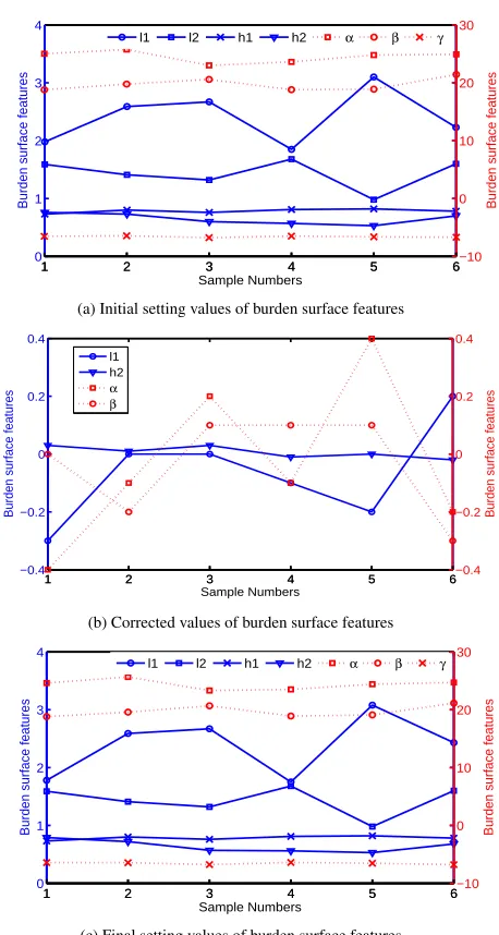
and 11(b). The results in Fig. 11(a) indicate that the burden surface features vary with the change of the production states. From Fig. 11(b), it can be seen that the corrected values change uncertainly according to the extracted rules, which may decrease, increase or unchange. Meanwhile, the final setting values after corrected are depicted in Fig. 11(c). Table V gives the optimal and actual values as well as upper and lower bounds of GUR and CR. As observed from Table V, the actual value of CR exceeds the upper bound under certain production condition, but the optimal values obtained by applying the proposed scheme is within the admissible ranges. Furthermore, the experimental results of two optimization algorithms used separately are shown in Table VI. According to Table VI, it can be observed that NSGA-II is more effective in determining the solutions than MOPSO for the first production situation and MOPSO obtains more optimal efficient solutions for the second production situation. The experimental results demon-strate that the proposed scheme can combine the advantages of the two algorithm to get a more efficient solution. Overall, it is obvious that optimal burden surface features improve the GUR and CR, which implies that the proposed scheme can provide reasonable burden surface parameters.
V. CONCLUSIONS
This paper presents an intelligent data-driven optimization scheme for determining the setting values of burden surface in the BF ironmaking process instead of manual operations. The salient features are nonlinear modeling of production
1 2 3 4 5 6
0 1 2 3 4
Sample Numbers
Burden surface features
1 2 3 4 5 6−10
0 10 20 30
Burden surface features
l1 l2 h1 h2 α β γ
(a) Initial setting values of burden surface features
1 2 3 4 5 6
−0.4 −0.2 0 0.2 0.4
Burden surface features
Sample Numbers
1 2 3 4 5 6−0.4
−0.2 0 0.2 0.4
Burden surface features
l1 h2 α β
(b) Corrected values of burden surface features
1 2 3 4 5 6
0 1 2 3 4
Burden surface features
Sample Numbers
1 2 3 4 5 6−10
0 10 20 30
Burden surface features
l1 l2 h1 h2 α β γ
[image:11.612.327.556.181.610.2](c) Final setting values of burden surface features
Fig. 11. Burden surface features generated by the proposed scheme
TABLE VI
COMPARISON RESULTS OF DIFFERENT OPTIMIZATION METHODS
No. algorithm GUR CR
1
Actual value 48.70 413.39
The proposed scheme 49.38 391.88
NSGA-II 48.91 405.62
MOPSO 49.38 391.88
2
Actual value 49.85 393.16
The proposed scheme 50.58 383.04
NSGA-II 50.58 383.04
MOPSO 50.03 390.59
In the future, how to establish the interpretable multi-objective optimization model to make the described optimization prob-lems more transparent and how to verify the proposed scheme on the actual site should be addressed.
REFERENCES
[1] Y. J. Li, S. Zhang, Y. X. Yin, J. Zhang, and W. D. Xiao, “A soft sensing scheme of gas utilization ratio prediction for blast furnace
via improved extreme learning machine,”Neural Process. Lett., 2018,
https://doi.org/10.1007/s11063-018-9888-3.
[2] J. Q. An, J. L. Zhang, M. Wu, J. H. She, and T. Terano, “Soft-sensing method for slag-crust state of blast furnace based on two-dimensional
decision fusion,”Neurocomputing, vol. 315, pp. 405-411, 2018.
[3] D. F. Xiao, J. Q. An, Y. He, and M. Wu, “The chaotic characteristic
of the carbon-monoxide utilization ratio in BF,”ISA Trans., vol. 68, pp.
109-115, 2017.
[4] M. Wu, K. X. Zhang, J. Q. An, J. H. She, and K. Z. Liu, “An energy efficient decision-making strategy of burden surface for blast furnace,”
Control Eng. Pract., vol. 78, pp. 186-195, 2018.
[5] P. K. Gupta, A. S. Rao, V. R. Sekhar, M. Ranjan, and T. K. Naha, “Burden distribution control and its optimization under high pellet operation,”
Ironmak. Steelmak., vol. 37, no. 3, pp. 235-239, 2010.
[6] P. Zhou, H. D. Song, H. Wang, and T. Y. Chai, “Data-driven nonlinear subspace modeling for prediction and control of molten iron quality
indices in blast furnace ironmaking,”IEEE Trans. Control Syst. Technol.,
vol. 25, no. 5, pp. 1761-1774, 2017.
[7] H. Saxen, C. H. Gao, and Z. W. Gao, “Data-driven time discrete models for dynamic prediction of the hot metal silicon content in the blast
furnace-A review,”IEEE Trans. Ind. Informat., vol. 9, no. 4, pp.
2213-2225, 2013.
[8] J. P. Li, C. C. Hua, Y. N. Yang, and X. P. Guan, “Fuzzy classifier design for development tendency of hot metal silicon content in blast furnace,”
IEEE Trans. Ind. Informat., vol. 14, no. 3, pp. 1115-1123, 2018.
[9] L. Jian and C. H. Gao, “Binary coding SVMs for the multiclass problem
of blast furnace system,”IEEE Trans. Ind. Electron., vol. 60, no. 9, pp.
3846-3856, 2013.
[10] Q. Liu, S. J. Qin, and T. Y. Chai, “Unevenly sampled dynamic data
modeling and monitoring with an industrial application,”IEEE Trans.
Ind. Informat., vol. 13, no. 5, pp. 2203-2213, 2017.
[11] G. L. Zhao, S. S. Cheng, W. X. Xu, and L. Chao, “Comprehensive math-ematical model for particle flow and circumferential burden distribution in charging process of bell-less top blast furnace with parallel hoppers,”
ISIJ Int., vol. 55, no. 12, pp. 2566-2575, 2015.
[12] P. Y. Shi, P. Zhou, D. Fu, and C. Q. Zhou, “Mathematical model for
burden distribution in blast furnace,”Ironmak. Steelmak., vol. 43, no. 1,
pp. 74-81, 2016.
[13] X. L. Li, D. X. Liu, C. Jia, and X. Z. Chen, “Multi-model control of
blast furnace burden surface based on fuzzy SVM,”Neurocomputing, vol.
148, pp. 209-215, 2015.
[14] T. Y. Chai, Z. X. Geng, H. Yue, H. Wang, and C. Y. Su, “A hybrid
intelligent optimal control method for complex flotation process,”Int J.
Syst. Sci., vol. 40, no. 9, pp. 945-960, 2009.
[15] W. Dai, T. Y. Chai, and S. X. Yang, “Data-Driven optimization control
for safety operation of hematite grinding process,” IEEE Trans. Ind.
Electron., vol. 62, no. 5, pp. 2950-2941, 2015.
[16] J. L. Ding, H. Modares, T. Y. Chai, and F. L. Lewis, “Data-based mul-tiobjective plant-wide performance optimization of industrial processes
under dynamic environments,” IEEE Trans. Ind. Informat., vol. 12, no.
2, pp. 454-465, 2016.
[17] J. F. Qiao and W. Zhang, “Dynamic multi-objective optimization control
for wastewater treatment process,” Neural Comput. Appl., vol. 29, pp.
1261-1271, 2018.
[18] J. D. Wei, X. Z. Chen, J. R. Kelly, and Y. Z. Cui, “Blast furnace stockline
measurement using radar,”Ironmak. Steelmak., vol. 42, no. 7, pp.
533-541, 2015.
[19] C. H. Gao, L. Jian, and S. H. Luo, “Modeling of the thermal state change
of blast furnace hearth with support vector machines,”IEEE Trans. Ind.
Electron., vol. 59, no. 2, pp. 1134-1145, 2012.
[20] Y. J. Li, S. Zhang, Y. X. Yin, W. D. Xiao, and J. Zhang, “A novel online sequential extreme learning machine for gas utilization ratio prediction
in blast furances,”Sensors, vol. 17, no. 4, pp. 1847-1870, 2017.
[21] P. Zhou, Y. Lv, H. Wang, and T. Y. Chai, “Data-driven robust RVFLNs modeling of a blast furnace iron-making process using Cauchy
distribu-tion weighted M-estimadistribu-tion,”IEEE Trans. Ind. Electron., vol. 64, no. 9,
pp. 7141-7151, 2017.
[22] L. Jian and C. H. Gao, “Binary coding SVMs for the multiclass problem
of blast furnace system,”IEEE Trans. Ind. Electron., vol. 60, no. 9, pp.
3846-3856, 2013.
[23] P. Zhou, C. Y. Wang, M. J. Li, H. Wang, Y. J. Wu, and T. Y. Chai, “Modeling error PDF optimization based wavelet neural network model-ing of dynamic system and its application in blast furnace ironmakmodel-ing,”
Neurocomputing, vol. 285, pp. 167-175, 2018.
[24] J. Q. An, J. Y. Yang, M. Wu, J. H. She, and T. Terano, “Decoupling
Control method with fuzzy theory for top pressure of blast furnace,”IEEE
Trans. Contr. Syst. Technol., DOI: 10.1109/TCST.2018.2862859, 2018.
[25] T. Mitra, F. Pettersson, H. Saxen, and N. Chakraborti, “Blast furnace charging optimization using multi-objective evolutionary and genetic
algorithms,”Mater. Manuf. Process., vol. 32, no. 10, pp. 1179-1188, 2017.
[26] Y. J. Li, S. Zhang, Y. X. Yin, W. D. Xiao, and J. Zhang, “Parallel one-class extreme learning machine for imbalance learning
based on Bayesian approach,” J. Amb. Intell. Hum. Comp., 2018,
https://doi.org/10.1007/s12652-018-0994-x.
[27] H. Saxen and F. Pettersson, “Nonlinear prediction of the hot metal silicon
content in the blast furnace,”ISIJ Int., vol. 47, pp. 1732-1737, 2007.
[28] Z. J. Liu, J. L. Zhang, and T. J. Yang, “Low carbon operation of
super-large blast furnaces in China,” ISIJ Int., vol. 55, no. 6, pp. 1146-1156,
2015.
[29] J. Zhang, W. D. Xiao, Y. J. Li, and S. Zhang, “Residual compensation
extreme learning machine for regression,”Neurocomputing, vol. 311, pp.
126-136, 2018.
[30] X. J. Lu, C. Liu, and M. H. Huang, “Online probabilistic extreme learning machine for distribution modeling of complex batch forging
processes,” IEEE Trans. Ind. Informat., vol. 11, no. 6, pp. 1277-1286,
2015.
[31] W. D. Xiao, J. Zhang, Y. J. Li, S. Zhang, and W. D. Yang, “Class-specific cost regulation extreme learning machine for imbalanced classification,”
Neurocomputing, vol. 261, pp. 70-82, 2017.
[32] G. B. Huang, H. M. Zhou, X. J. Ding, and R. Zhang, “Extreme learning
machine for regression and multiclass classification,”IEEE Trans. Syst.
Man Cybern. Part B Cybern., vol. 42, no. 2, pp. 513-529, 2012.
[33] K. Deb, A. Pratap, S. Agarwal, and T. Meyarivan, “A fast and elitist
multiobjective genetic algorithm NSGA-II,”IEEE Trans. Evolut. Comput.,
vol. 6, no. 2, pp. 182-197, 2002.
[34] C. A. Coello, G. T. Pulido, and M. S. Lechuga, “Handing multiple
ob-jective with particle swarm optimization,”IEEE Trans. Evolut. Comput.,
vol. 8, no. 3, pp. 256-279, 2004.
[35] C. L. Hwang and K. Yoon, “Multiple attribute decision making: methods and applications,” Berlin: Springer, 1981.
[36] H. C. Peng, F. H. Long, and C. Ding, “Feature selection based on mutual information: criteria of max-dependency, max-relevance, and
min-redundancy,”IEEE Trans. Pattern Anal. Mach. Intell., vol. 27, no. 8, pp.
Yanjiao Li is a Ph.D. candidate with the School
of Automation&Electrical Engineering, University
of Science and Technology Beijing, P.R. China. Currently, she is also a visiting research fellow with the School of Electronic and Electrical Engineering, University of Leeds, U.K. Her research interests in-clude machine learning, modeling and optimization for complex systems.
Sen Zhangreceived the Ph.D. degree from Nanyang Technological University, Singapore, in 2005 and worked as a postdoctoral research fellow in National University of Singapore and lecturer in charge with Singapore Polytechnic. She is currently an
asso-ciate professor with the School of Automation&
Electrical Engineering, University of Science and Technology Beijing, P.R. China. Her research inter-ests include machine learning, target tracking and estimation theory.
Jie Zhang is a Ph.D. candidate with the School
of Automation&Electrical Engineering, University
of Science and Technology Beijing, P.R. China. Currently, he is also a visiting research fellow with the School of Electronic and Electrical Engineering, University of Leeds, U.K. His research interests in-clude machine learning, deep learning, and wireless sensor networks.
Yixin Yinreceived the B.S., M.S., Ph.D. degrees from University of Science and Technology Bei-jing, P.R. China, in 1982, 1984, 2002, respectively. Currently, he is a full professor with the School of
Automation&Electrical Engineering, University of
Science and Technology Beijing, P.R. China. Prof. Yin is a fellow of Chinese Society for Artificial In-telligence, and a member of the Chinese Society for Metals and the Chinese Association of Automation. His research interest includes modeling and control for complex systems and artificial life.
Wendong Xiao (M’01-SM’09)received the Ph.D. degree from Northeastern University, P.R. China, in 1995. Currently, he is a professor with the School
of Automation&Electrical Engineering, University
of Science and Technology Beijing, P.R. China. Previously, he hold various academic and research positions with Northeastern University (P.R. China), POSCO Technical Research Laboratories (South Ko-rea), Nanyang Technological University (Singapore), and the Institute for Infocomm Research, A*STAR (Singapore). His current research interests include machine learning, big data processing, wireless localization and tracking, ener-gy harvesting based network resource management, wireless sensor networks and internet of things.