An evaluation approach for a physically-based sticky lip model

White Rose Research Online URL for this paper:

http://eprints.whiterose.ac.uk/143406/

Version: Published Version

Article:

Leach, M. and Maddock, S. orcid.org/0000-0003-3179-0263 (2019) An evaluation

approach for a physically-based sticky lip model. Computers, 81 (1). 24. ISSN 2073-431X

https://doi.org/10.3390/computers8010024

[email protected] https://eprints.whiterose.ac.uk/ Reuse

This article is distributed under the terms of the Creative Commons Attribution (CC BY) licence. This licence allows you to distribute, remix, tweak, and build upon the work, even commercially, as long as you credit the authors for the original work. More information and the full terms of the licence here:

https://creativecommons.org/licenses/

Takedown

If you consider content in White Rose Research Online to be in breach of UK law, please notify us by

Article

An Evaluation Approach for a Physically-Based

Sticky Lip Model

†

Matthew Leach *,‡ and Steve Maddock‡

The Department of Computer Science, University of Sheffield, Regent Court, 211 Portobello, Sheffield S1 4DP, UK; [email protected]

* Correspondence: [email protected]

† This paper is an extended version of conference paper “Leach, M.; Maddock, S. Physically-based Sticky Lips. In Proceedings of the EG UK Computer Graphics and Visual Computing, EGUK, Swansea, Wales,

13–14 September 2018”.

‡ These authors contributed equally to this work.

Received: 18 January 2019; Accepted: 5 March 2019; Published: 8 March 2019

Abstract:Physically-based mouth models operate on the principle that a better mouth animation will be produced by simulating physically accurate behaviour of the mouth. In the development of these models, it is useful to have an evaluation approach which can be used to judge the effectiveness of a model and draw comparisons against other models and real-life mouth behaviour. This article presents a set of metrics which can be used to describe the motion of the lips, as well as a process for measuring these from video of real or simulated mouths, implemented using Python and OpenCV. As an example, the process is used to evaluate a physically-based mouth model focusing on recreating the stickiness effect of saliva between the lips. The metrics highlight the changes in behaviour due to the addition of stickiness between the lips in the synthetic mouth model and show quantitatively improved behaviour in relation to real mouth movements. The article concludes that the presented metrics provide a useful approach for evaluation of mouth animation models that incorporate sticky lip effects.

Keywords:evaluation; facial animation; physically-based; sticky lips

1. Introduction

The mouth is one of the key areas in producing a convincing animation of a face, such as in visual speech applications. Humans are acutely aware of its movement. The fine details of this are therefore important to capture. One contributing factor to these movements is the stickiness of the lips, which can vary with time and position on the lips. For example, a slow separation of the lips may produce multiple mouth openings as the lips separate, or produce asymmetric behaviour, and a plosive speech action may cause the mouth to appear to stick before bursting open. These effects are difficult to recreate with traditional facial animation approaches. A physically-based approach is required. Physically-based facial animation approaches seek to model the underlying physical behaviour of the materials involved to reproduce realistic behaviour.

In our previous work [1], we used a finite-element based approach to mimic the behaviour of the mouth. This work incorporates a model of saliva. The saliva between the lips acts as a glue as it dries out, bonding the two lips through adhesive forces sticking the saliva to the lips and internal cohesive forces sticking the saliva to itself. This physically-based recreation supports varying degrees of stickiness, dynamic effects as the cohesive layer breaks under tension, time varying behaviour and asymmetric effects. Such sticky effects are absent or must be heuristically added to blend shape approaches, which makes it difficult to accurately model the potentially infinite range of behaviours that sticky saliva can create on the lips.

These often subtle effects of saliva on the lips are difficult to evaluate using typical objective methods. Current model fitting approaches do not deal with multiple mouth openings, caused as parts of the lips stick together. Whilst subjective evaluation methods may be able to judge plausibility, it is nonetheless useful to have an objective measure of correctness. As such, we propose an evaluation process consisting of a set of metrics and an algorithm for extracting them from video using image processing, which provides information on the shape and number of mouth openings and the way they change over time. The process is used to evaluate the effectiveness of the inclusion of the sticky lip effect in a finite element model. The results show that the profiles of the graphs generated from these data compare well with real mouth sticky behaviour and also give insight into the way the mouth behaves. They suggest that the inclusion of the sticky lip effect is important for producing realistic mouth opening behaviour.

The remainder of the paper is organised as follows. Section2gives an overview of literature for production and evaluation of mouth animations. Section3describes the creation of the model used to generate the mouth animations which are evaluated in this paper. Section4details the evaluation process. Section5presents and discusses the results. Finally, Section6gives the conclusions.

2. Related Work

Much computer facial animation work has been concerned with animation of the face as a whole. Early work used simple transformations and interpolation between expressions [2]. Subsequent approaches used volume modelling [3,4] with some producing muscle simulations [5–9]. More recently, hybrid models have combined physically-based approaches with other techniques [10–12]. The current industry standard techniques are motion capture, markerless [13] or marker-based [14], and blendshape animation, based on extreme poses calledblend targets, where each blend target typically encodes one action, such as raising an eyebrow, and multiple blend targets can be linearly combined.

Hybrid approaches build on the blend shapes idea. Blend forces [10] encode forces to drive a physically-based model, rather than encoding blendshape displacements directly. This allows more advanced physical interactions including better lip response due to collision. Cong et al. [11] combined a physically-based simulation with blendshapes to allow artist direction. Artists can influence the movement of particular muscles with blendshapes, whilst the remainder of the animation is completed using the physical model. Kozlov et al. [12] also used a hybrid approach, overlaying a physical simulation on blendshape based animations, in which secondary motions caused by dynamics can be reintroduced. Ichim et al. [15] used a physics-based model with a novel muscle activation model and detect contact between the lips using axis-aligned bounding box hierarchies. This improves lip behaviour, but still does not deal with stickiness during separation of the lips.

The “sticky lip problem” is a term describing the way the lips stick together due to moisture as they are drawn apart. Modelling this behaviour could improve visual realism when creating characters who are chewing, or for accurate plosive effects in visual speech, or could be used in cases where hyper-realism is required. In academia, the sticking of the lips is described as “difficult to attain with existing real-time facial animation techniques” [16]. Olszewski et al. approached this problem using a motion capture system which produces convincing results, but is not easy to edit for an artist. The system uses a trained convolutional neural network to learn parameters controlling a digital avatar. The Digital Emily project [17] states that the problem has been modelled in various facial rigs, including the character Gollum in The Lord of the Rings, further demonstrating the desire for a good solution.

mouth opens. Our stickiness model improves on his probability based model, providing a deterministic behaviour grounded in physics.

Whichever mouth animation approach is chosen, evaluation must be done. The most common quantitative evaluation approach is to use a ground truth distance measured against marker-based motion capture or markers located in video. This approach is used in various papers using a variety of modelling techniques (e.g., [10,20]). Although this does provide an objective measure of how close the animation is to the original movements of the face, subtle effects which may be important to the plausibility of an animation may have little impact on the ground truth distance average.

Other analysis methods make use of active appearance or active shape models (AAM/ASM) [21–24]. These methods aim to statistically fit a shape or model to a new image based on trained data. This approach is used in the software Faceware Analyzer [25]. As these approaches rely on fitting a predefined shape (typically the inner and outer lip contours), they are not well suited to tracking the dynamic behaviours which appear as a result of the sticky lips, since this may involve multiple mouth openings as the lips stick together in different places.

The alternative to quantitative analysis is human perception studies, where participants make judgments about the quality of the results (e.g., [26,27]). These are commonly used, backed up by the reasoning that humans are the best judge of any animation results. Although such tests can be effective for evaluating plausibility, in establishing whether or not behaviour is physically correct, it is useful to have an objective measure. We present such an approach in this paper.

3. A Physically-Based Mouth Model

Our previous work implemented a physically-based mouth model using the TLED approach [1]. This section gives a summary of that work, since the results are used in the subsequent evaluation process, and it is important to understand what processes the model includes.

The face model was created using a combination of FaceGen [28] and Blender [29]. An initial model, based on photographs of the first author, was created in FaceGen. This model was exported to Blender, where the teeth, tongue, and large portions of the face were removed to leave the lower, front half of the face. This process does not produce a perfect recreation of the user’s face, for example there are some discrepancies between the lip shapes of the real person and the model. However, this does not impact on the work in this paper as we are interested in the overall behaviour of the mouth, particularly the timing of dynamic events such as lips parting, rather than accurately recreating a single person’s mouth. Different material regions—skin and a thin saliva layer between the lips—were then defined using Blender’s material feature, as shown in Figure1. A bespoke program was then used to extrude the quads of the surface mesh into hexahedra, as under-integrated linear hexahedral elements are used in the finite element simulation. The final model consists of 3414 hexahedral elements.

As the focus of the work is on recreation of the stickiness of the lips, a simple muscle model is used for producing mouth motion. Linear virtual vector muscles are used to control the mesh around the mouth. Only the muscles providing the biggest effect on the movement of the mouth are modelled. Muscles are defined by an origin point, an insertion point, and a radius. Collectively, these variables define a cylinder. The forces generated by the muscle are applied to all points within the cylinder and act in a uniform direction along the length of the muscle.

Figure 1.Material definitions in the modelling package Blender. Blue and red represent normal soft tissue and green represents the saliva layer.

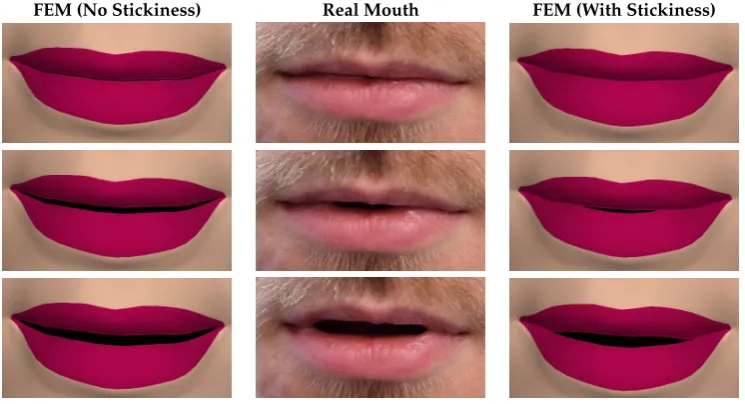
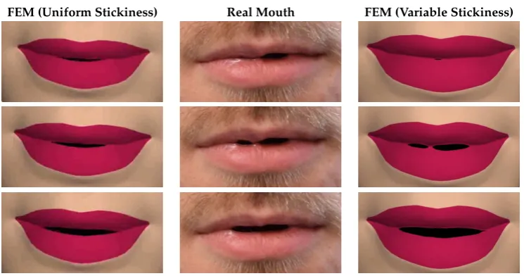
For the animations including sticky saliva, the saliva is represented by a thin layer of finite elements between the lips. These elements are capable of stretching and breaking once they reach a certain stretch, based on the moisture level on the lips. Figures2–4demonstrate some of the effects the model is capable of producing. Figure2shows the mouth opening over time, and how the zippering occurs from the centre. Figure3demonstrates the formation of multiple mouth openings due to a central sticky area on the lips. Figure4shows that the model can easily be texture mapped, although for clarity and more effective analysis, the majority of the images throughout the paper are untextured.

FEM (No Stickiness) Real Mouth FEM (With Stickiness)

FEM (Uniform Stickiness) Real Mouth FEM (Variable Stickiness)

Figure 3. A comparison of an animation produced by: a finite element model without stickiness (left column); a real mouth (middle column); and a finite element model with stickiness, where a point near the centre of the mouth is stuck, producing multiple mouth openings (right column). The stickiness provides a much more realistic movement of the lips throughout the animation. Time progresses vertically down the page with a 0.12 s interval between each row.

Figure 4.(Left) Real mouth; and (Right) texture mapped mouth with physically-based sticky lips.

The simulation component of the animation was conducted using the software NiftySim [30], which is designed for soft tissue simulation. NiftySim uses the total Lagrangian explicit dynamics (TLED) formulation of the finite element method. This formulation presents various advantages for this work. A total formulation always computes timesteps relative to the initial state, allowing significant precomputation. In addition, this formulation is highly parallel as element forces can be computed in parallel—without this, the approach would be prohibitively computationally expensive on standard hardware. Many other formulations of the finite element method can not be solved in parallel in this way. The use of a dynamic formulation is essential as we are looking at producing an animation; static or quasi-static formulations aim to simulate the correct equilibrium behaviour, but do not accurately model the intermediate steps which are necessary for creating an animation rather than just a final pose.

A full analysis of the method and techniques used is available in [30]. The fundamentals are briefly presented here. In the total formulation, deformations are computed with respect to the initial configuration. We are also interested in large deformations. This makes the Green–Lagrange strain tensor and its work-conjugate, the second Piola–Kirchoff stress tensor, appropriate choices. From the principle of virtual work, the problem can be stated as:

Z

0_VSδEdV=

Z

0_Vδu f

(B)_d0_V+Z

0_Sδu f

(S)_d0_{S (1)}

with respect to the initial configuration; the body and surface force vectors are those at timet; andδu, the virtual displacements, are also considered at timet.

This continuous domain is approximated by a series of discrete elements. Variation of physical properties over the elements is represented through shape functions. A strain–displacement matrix is used to relate strains across an element with displacements of the nodes. Through application of the prior formulae to each degree of freedom, the principle of virtual work leads to the equation of motion:

M tu¨+Ctu˙+k(tu) tu= tr (2)

where, for an elementt,uis the vector of displacements,Mis the lumped (diagonal) mass matrix,Cis the damping matrix,k(t_{u)is the element stiffness matrix, and}t_{ris the external force vector. This is}

solved to obtain the forces for each element using the second Piola–Kirchoff tensor:

f(e)=8det(J)δhSFT (3)

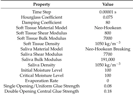
where f(e)is the internal force for an elemente, Jis the element Jacobian matrix,δhare the shape function derivatives,Sis the second Piola–Kirchoff stress tensor, andFis the deformation gradient. Boundary conditions are imposed, and the simulation is advanced using the central difference integrator for time. A neo-Hookean material model is used. The moisture model includes evaporation and variable stickiness based on the moisture level. Full details can be found in the previous paper [1]. The parameter values used are listed in Table1.

Table 1.The parameters used to generate the results shown in Figures2and3.

Property Value

Time Step 0.00001 s

Hourglass Coefficient 0.075

Damping Coefficient 80

Soft Tissue Material Model Neo-Hookean

Soft Tissue Shear Modulus 800

Soft Tissue Bulk Modulus 7000

Soft Tissue Density 1050 kg/m−3

Saliva Material Model Neo-Hookean Breaking

Saliva Shear Modulus 7700

Saliva Bulk Modulus 191,000

Saliva Density 1050 kg/m−3

Initial Moisture Level 100

Critical Moisture Level 100

Evaporation Rate 0

Single Opening/Uniform Glue Strength 0.08 Double Opening Central Glue Strength 0.18

4. The Evaluation Process

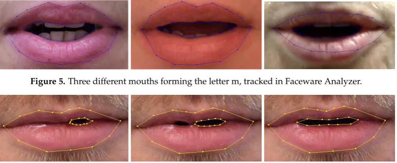
Figure 5.Three different mouths forming the letter m, tracked in Faceware Analyzer.

Figure 6.(Left) Faceware Analyzer correctly detects the outer lip contour and the inner lip contour for a single mouth opening; (Middle) Faceware Analyzer correctly detects the outer lip contour, but can only detect one of the two mouth openings present; and (Right) once the mouth openings merge, Faceware Analyzer correctly detects the outer and inner lip contours.

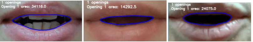
Given the problems of detecting multiple mouth openings, as might be produced in a sticky lips model, a new evaluation approach is needed to analyse these effects. We propose four metrics to capture information about the openings of sticky lips:

• Number of Mouth Openings: The number of individual mouth openings.

• Mouth Opening Area: The mouth opening area is the area contained within a mouth

opening contour.

• Mouth Opening Width: The mouth opening width is computed as the difference between the

greatest and least x coordinates of pixels that lie within a mouth opening.

• Mouth Opening Height: The mouth opening height is computed as the difference between the

greatest and least y coordinates of pixels that lie within a mouth opening.

The number of mouth openings is a metric designed to capture the subtle effects produced by sticky lips—effects we believe add to the realism of mouth movement. The width and height of mouth openings provides considerable information about the way the mouth is opening, particularly when examined over time. These give direct information about how the shape of the mouth opening is changing, while jumps in mouth width show exactly when two openings combine as stuck portions of the lips come unstuck.

The movement of the human mouth also takes place over a range of time scales. As such, each of the metrics considered are examined over time. This is particularly important for capturing potential dynamic effects. A model may reach the same equilibrium position or move through identical key frames as a real mouth, but might not capture the movements in between correctly. Additionally, plosives and other such highly dynamic movements take place very quickly. Whilst they are difficult to judge by eye, they cause dynamic effects in the lips which are important for realism. The metrics profiles over time, and their derivatives, can give useful information about whether or not a synthetic facial animation approach is similar to the behaviour of a real mouth.

To ensure consistency across face sizes, mouth widths, etc., the metrics are normalised against the natural mouth width. This has been defined as the distance in pixels between the corners of the mouth at rest. Each value recorded is divided by the natural mouth width. This allows comparison between different videos.

1. Convert to greyscale 2. Blur

3. Threshold

4. Contour detection

5. Sorting/Region identification 6. Metric extraction

Figure7shows the process for a single mouth opening. The source image is first converted to greyscale to simplify the thresholding process. This is done using the rec601 luma conversion [31].

Y=0.299r+0.587g+0.114b (4)

whereYis the greyscale value,ris the red channel value,gis the green channel value andbis the blue channel value for a given pixel.

The greyscale image is blurred using a standard median blur to prevent small dark spots in the image from being falsely identified as mouth openings. The specific kernel width used varies depending on the width of the mouth in pixels, as the scale is important. A kernel width of 11 was found to provide a good balance between retaining detail and removing false positives for a mouth width of around 800 pixels, measured at rest from corner to corner horizontally.

(a) (b) (c)

(d) (e)

Figure 7.(a) Source frame; (b) greyscale version; (c) greyscale image blurred with 11 px median filter; (d) segmentation based on brightness threshold, where the mouth opening is identified by the white pixels; and (e) contour of edge of segmented mouth opening overlaid on original source image.

The thresholding process aims to identify mouth opening regions. As the aim is classifying pixels as mouth opening or not mouth opening, a binary threshold is used. The final stage of mouth opening detection is to identify the contours which form the boundaries of each segmented region. The contour detection is implemented using OpenCV’s findContours, which uses the method described by Suzuki et al. [32].

The approach works well for synthetic mouths, as illustrated in Figure8, which shows the boundary detection process for a synthetic mouth with multiple openings. The image contains no noise and is trivial to track, unlike a real mouth. For a real mouth, boundary detection can be less accurate due to reflections from the inside of the mouth or the teeth or tongue appearing a similar brightness to the lips.

Figure 8.The lips can be seen separating in some places, but still stuck in places where the stickiness is higher. The analysis shows that two mouth openings are detected.

Figure 9.The convex hull of the contour provides a very good approximation of the correct lip contour.

Another issue is that small specular reflections inside the mouth can be falsely identified as openings. This is resolved by blurring the image to remove small highlights and noise, and then only keeping top level contours in the contour hierarchy. A further issue is that, in some lighting conditions and mouth positions, the teeth are sufficiently bright and visible to be detected as part of the lips. Only a partial solution to this problem has been developed. Figure10a shows the mouth without the teeth detection enabled. To solve this, the image is further converted to the HSV colour space, in which white and black are easily distinguishable from other colours (Figure10b). Further segmentation detects the teeth (Figure10c). This mask is then subtracted from the original greyscale image to darken the teeth, leading them to be included in the mouth opening rather than the lip region (Figure10d). This process is not always reliable and could present an interesting area for future work. Liévin et al.’s statistical approach to segment the mouth area, making use of red hue and motion, could be considered [33].

(a) (b)

(c) (d)

Figure 10. (a) Frame with no teeth detection; (b) source frame transformed to HSV colour space; (c) segmentation based on saturation channel; and (d) updated frame with teeth detection.

mouth, respectively. This distance then functions as the normalisation width. All the measurements are divided by this to ensure consistency across video resolutions and mouth sizes. This box is also used to crop the video to the mouth area. (Figure11). This is the only manual stage. Thereafter, the process is automatic. The analysis process is then carried out for each frame of the video with each metric being computed and the results stored. When all videos have been analysed, derivatives of the opening width and area are computed by taking the differences between each frame. Graphs are then generated using Matplotlib.

Figure 11.The mouth area selection box is aligned with the corners of the mouth. This selects the video region for analysis and the width of the box is used to normalise the collected data.

5. Results and Discussion

To evaluate the effect the stickiness has on the finite element model, two different cases of lip stickiness were examined. The first case was a single mouth opening with the lip “unzippering” from the centre. Here, a real mouth, a physically-based lip model without stickiness and a physically-based lip model with stickiness were compared. The second case was two mouth openings, with the saliva causing the lips to be stuck near to the centre of the mouth. Here, a real mouth, the physically-based lip model with uniform stickiness in which all saliva elements have the same moisture level, and the physically-based lip model with variable stickiness in which a central element has increased stickiness were compared. The aim was to show that our sticky lip model gave a closer match to the real lip behaviour, with the emphasis on the timing of events such as lip separation. The first case demonstrated the basic effect of including stickiness. The second case showed how the stickiness/moisture model can be used to reproduce more advanced effects.

The real mouth videos were recorded using a Nikon D3300 camera, set to record at 60 fps. The camera was mounted on a tripod to ensure a consistent location of the mouth within the footage by minimising shaking. The participant was seated in front of the tripod in a well lit room at a distance of roughly 1 m from the camera. The footage captured the lower half of the face, and featured the participant performing a range of mouth movements. Prior to and at certain points throughout the recording, the lips were licked, leading to varying levels of stickiness throughout the recordings. Videos of the simulated mouths were recorded using OBS Studio screen recording software [34].

5.1. Detecting Mouth Openings

Figure13c shows an example which combines the use of the convex hull and the teeth detection to capture the inner lip contour well despite difficult lighting conditions and the presence of bright teeth next to the lip. Figure13d shows how the mouth opening can be correctly detected even for situations where the tongue is protruding as when licking the lips. Traditional approaches would struggle to correctly determine the inner lip contour here.

Figure 12.Three mouths forming the letter m, tracked in our analysis tool.

(a) (b)

(c) (d)

Figure 13.(a) Inner lip contour is accurately detected despite the bright tongue; (b) inner lip contour is very clearly defined as there is good contrast between the mouth opening and lips; (c) the tooth detection and convex hull approach provide a good estimate of the inner lip contour; and (d) even in traditionally challenging mouth positions such as the tongue protruding whilst licking the lips, mouth openings are detected.

FEM (No Stickiness) Real Mouth FEM (With Stickiness)

Figure 14. Analysis of an animation produced by: a finite element model without stickiness (left column); a real mouth (middle column); and a finite element model with stickiness (right column). Time progresses vertically down the page with a 0.12 s interval between each row.

Figure15shows the detection process for two mouth openings. This shows the analysis for the frames in Figure3. In these frames, the top row has a small single mouth opening. In the second row, a central portion of the lip with higher stickiness causes a second mouth opening to form in the case of the real mouth. The variable stickiness model (right hand column of Figure15) recreates this effect, whilst with uniform stickiness (left hand column of Figure15) only a single mouth opening forms. In the final row, the stuck saliva has broken and a single mouth opening is present.

FEM (Uniform Stickiness) Real Mouth FEM (Variable Stickiness)

Figure 15. Analysis of an animation produced by: a finite element model without stickiness (left column); a real mouth (middle column); and a finite element model with stickiness (right column). This example shows two mouth openings. Time progresses vertically down the page with a 0.12 s interval between each row.

5.2. Opening over Time

for a range of mouth movements across three people. Figure16shows three people pronouncing the plosive letter “m” (as in the word “mum”). The graphs show similar profiles, but different opening speeds are apparent, showing the individuality of each speaker. Figure17shows the same three people saying the word “baby”. The two plosive pronunciations of “b” are clear, again showing the similarities as well as the individuality of each speaker.

Speaker 1 Speaker 2 Speaker 3

Figure 16.Graphs showing the opening profiles for three different speakers producing an “m” sound. The top row shows the area, the middle row shows opening width and the bottom row shows the opening height.

Speaker 1 Speaker 2 Speaker 3

Figure 17.Graphs showing the opening profiles for three different speakers speaking the word “baby”. The top row shows the area, the middle row shows opening width and the bottom row shows the opening height.

Figure21shows graphs for Barrielle and Stoiber’s model [19], where the mouth opens twice. The graph was generated from a portion of the video accompanying their paper [19]. These results show similarities to our work. However, the stochastic behaviour in their model is also shown, as the two profiles in each graph are not identical.

Figure 19.For a typical mouth opening action where only a single mouth opening forms, the inclusion of stickiness matches the opening height profile of the real mouth much better than without stickiness. The real mouth and sticky model both initially open slowly and then more quickly as time progresses. The non-sticky model opens quickly initially and then tapers off.

Figure15examines the metrics tracked over a mouth opening action in which multiple mouth openings form. Double mouth opening simulations use increased stickiness on one of the central elements. Figures22–24show the graphs that are produced from the analysis. A particularly sticky section near the centre of the lip remains stuck momentarily as the lips are drawn apart. This causes two mouth openings to be present temporarily until the stuck section breaks at around frame 45. Following this, there is a single mouth opening present. The graphs track properties for the largest mouth opening, so when the saliva breaks, jumps in the value of particular metrics are often noticeable. This provides information about when the saliva is breaking apart and shows the effect of the split on the behaviour of the mouth.

Figure 21. Graphs showing the effect of Barrielle and Stoiber’s sticky lip model [19] opening the mouth twice.

In Figure 22, the sharp jump in opening width at the 45 frame mark in the real and sticky simulations is absent from the simulation without stickiness, as with no stickiness only a single mouth opening forms. Aside from this distinct feature, the sticky simulation also matches the profile of the real mouth more closely than the non-sticky simulation for the first portion of the videos. Both the real and sticky profiles feature a fairly sharp initial rise in mouth opening (Figure23), which then tapers off until frame 45 when the saliva breaks. At this point, both the real and sticky profiles again feature a sharp rise. The non-sticky simulation’s opening width rises much more smoothly. In Figure24, there is a sudden step up in the area when the saliva breaks in both the sticky and real simulations.

Figure 23.Both the real and sticky profiles feature a fairly sharp initial rise in mouth opening height, which then tapers off until frame 45 when the saliva breaks. At this point, both the real and sticky profiles again feature a sharp rise. The non-sticky simulation’s opening width rises much more smoothly.

Figures25 and26show the area and opening width derivative graphs, respectively, for the multiple mouth opening example. These graphs strongly identify points at which mouth openings combine as the saliva breaks. Sharp spikes can be clearly seen in the real and sticky mouths around frame 45, while this spike is absent in the non-sticky mouth model.

Figure 25.This graph shows the derivative of the area over time. The sharp spike in area can be very clearly seen here in the real and sticky mouths, but is absent in the non-sticky mouth model.

Figure 26.This graph shows the derivative of the opening width over time. There is a sharp spike in opening width at frame 45 for the real and sticky mouths (although the green line mostly obscures the orange line), but this is absent in the non-sticky mouth model.

5.3. Discussion

The rate of evaporation of a fluid from a surface is given by the Herz–Knudsen equation:

1

A dN

dt ≡ϕ=

α(pliq−peq)

q

2πmkBTliq

(5)

whereAis the surface area of the fluid,Nis the number of gas molecules,ϕis the flux of gas molecules,

αis a sticking coefficient for the gas molecules onto the surface,pliq is the pressure of the liquid during

evaporation,peqis the liquid pressure at which an equilibrium between evaporation and condensation

is reached,mis the mass of a liquid particle,kBis the Boltzmann constant andTliqis the temperature

of the liquid.

Our model makes a series of assumptions surrounding these parameters, taking the pressures and temperatures as constant, as well as time-averaging the air speed over the lips. This gives a constant evaporation rate. For each element, an initial moisture level,0M, and a current moisture level at timet,

t_{M, are used. A moisture level of 0 represents a completely dry lip with a higher value representing}

more moisture. Thus, it follows that the moisture level at timetis given by:

t_M=

( ₀

M−tϕ if 0M>t_ϕ

0 otherwise (6)

Further work is required to investigate the validity of these assumptions, which could improve the moisture model and stickiness behaviour. The evaluation approach introduced in this paper could help with understanding this behaviour.

The current finite element approach can deal with simple collisions of the lips, as resistive forces are generated by compression of the saliva elements. However, a more rigorous model for collision between the lips could be developed. This would include shearing as the lips slide over each other. The teeth and tongue could then be added into the model and interactions with these could then be included.

The evaluation approach has demonstrated that it is useful for identifying the dynamic behaviour that accompanies the sticky lip effect. The graphs demonstrate the bursts of activity as multiple mouth openings merge, as well as show the gradual change in area as the mouth opens. However, there is room for improvement in the mouth opening detection process. As noted earlier, for a real mouth, reflections from the tongue and teeth are sometimes picked up and falsely identified as the lip area. This problem occurs when the mouth opens wider. Thus, it may be possible to use the more accurate detection process for small mouth openings to help predict the correct shape as the mouth opens further. Further work will also test the approach on a larger population of mouth motions.

6. Conclusions

Author Contributions:Investigation, M.L.; Methodology, M.L.; Software, M.L.; Supervision, S.M.; Validation, M.L.; Writing—original draft, M.L.; and Writing—review and editing, S.M.

Funding:This research was funded by the EPSRC.

Conflicts of Interest:The authors declare no conflict of interest. The funders had no role in the design of the study; in the collection, analyses, or interpretation of data; in the writing of the manuscript, or in the decision to publish the results.

Abbreviations

The following abbreviations are used in this manuscript:

TLED Total Lagrangian Explicit Dynamics FEM Finite Element Method

AAM Active Appearance Model ASM Active Shape Model

References

1. Leach, M.; Maddock, S. Physically-based Sticky Lips. In Proceedings of the EG UK Computer Graphics & Visual Computing, EGUK, Swansea, UK, 13–14 September 2018.

2. Parke, F.I. A model for human faces that allows speech synchronized animation.Comput. Graph.1975,1, 3–4.

[CrossRef]

3. Waters, K. Physical model of facial tissue and muscle articulation derived from computer tomography data. In Proceedings of the Visualization in Biomedical Computing, International Society for Optics and Photonics, Chapel Hill, NC, USA, 13–16 October 1992; pp. 574–583.

4. Lee, Y.; Terzopoulos, D.; Waters, K. Realistic modeling for facial animation. In Proceedings of the 22nd aNnual Conference on Computer Graphics and Interactive Techniques, Los Angeles, CA, USA, 6–11 August 1995; ACM: New York, NY, USA, 1995; pp. 55–62.

5. Waters, K. A Muscle Model for Animation Three-dimensional Facial Expression.SIGGRAPH Comput. Graph. 1987,21, 17–24. [CrossRef]

6. Ekman, P.; Friesen, W.V. Manual for the Facial Action Coding System; Consulting Psychologists Press: Palo Alto, CA, USA, 1978.

7. Chabanas, M.; Payan, Y. A 3D Finite Element Model of the Face for Simulation in Plastic and Maxillo-Facial Surgery. In Proceedings of the Medical Image Computing and Computer-Assisted Intervention, Pittsburgh, PA, USA, 11–14 October 2000; pp. 1068–1075.

8. Kahler, K.; Haber, J.; Seidel, H.P. Geometry-based Muscle Modeling for Facial Animation. In Proceedings of the Graphics Interface, Ottawa, ON, Canada, 7–9 June 2001; pp. 37–46.

9. Scheepers, F.; Parent, R.E.; Carlson, W.E.; May, S.F. Anatomy-Based Modeling of the Human Musculature. In Proceedings of the SIGGRAPH ’97, Los Angeles, CA, USA, 3–8 August 1997; ACM: New York, NY, USA, 1997. 10. Barrielle, V.; Stoiber, N.; Cagniart, C. BlendForces: A Dynamic Framework for Facial Animation.

Comput. Graph. Forum2016,35, 341–352. [CrossRef]

11. Cong, M.; Bhat, K.S.; Fedkiw, R. Art-directed muscle simulation for high-end facial animation. In Proceedings of the Symposium on Computer Animation, Zurich, Switzerland, 11–13 July 2016; pp. 119–127.

12. Kozlov, Y.; Bradley, D.; Bächer, M.; Thomaszewski, B.; Beeler, T.; Gross, M. Enriching Facial Blendshape Rigs with Physical Simulation.Comput. Graph. Forum2017,36, 75–84. [CrossRef]

13. Beeler, T.; Hahn, F.; Bradley, D.; Bickel, B.; Beardsley, P.; Gotsman, C.; Sumner, R.W.; Gross, M. High-quality passive facial performance capture using anchor frames.ACM Trans. Graph.2011,30, 75. [CrossRef] 14. Deng, Z.; Chiang, P.Y.; Fox, P.; Neumann, U. Animating blendshape faces by cross-mapping motion capture

data. In Proceedings of the 2006 Symposium on Interactive 3D Graphics and Games, Redwood City, CA, USA, 14–17 March 2006; ACM: New York, NY, USA, 2006; pp. 43–48.

15. Ichim, A.E.; Kadleˇcek, P.; Kavan, L.; Pauly, M. Phace: Physics-based face modeling and animation.

ACM Trans. Graph.2017,36, 153. [CrossRef]

16. Olszewski, K.; Lim, J.J.; Saito, S.; Li, H. High-fidelity facial and speech animation for VR HMDs.

17. Alexander, O.; Rogers, M.; Lambeth, W.; Chiang, M.; Debevec, P. The Digital Emily project: Photoreal facial modeling and animation. In Proceedings of the ACM SIGGRAPH 2009 Courses, Yokohama, Japan, 16–19 December 2009; ACM: New York, NY, USA, 2009; p. 12.

18. Gascón, J.; Zurdo, J.S.; Otaduy, M.A. Constraint-based simulation of adhesive contact. In Proceedings of the 2010 ACM SIGGRAPH/Eurographics Symposium on Computer Animation, Madrid, Spain, 2–4 July 2010; Eurographics Association: Aire-la-Ville, Switzerland, 2010; pp. 39–44.

19. Barrielle, V.; Stoiber, N. Realtime Performance-Driven Physical Simulation for Facial Animation.

Comput. Graph. Forum Wiley Online Libr.2018, doi:10.1111/cgf.13450. [CrossRef]

20. Cosker, D.; Marshall, D.; Rosin, P.L.; Hicks, Y. Speech driven facial animation using a hidden markov coarticulation model. In Proceedings of the Pattern Recognition, 17th International Conference on (ICPR’04), Cambridge, UK, 23–26 August 2010; IEEE: Washington, DC, USA, 2004; pp. 128–131.

21. Hill, A.; Cootes, T.F.; Taylor, C.J. Active shape models and the shape approximation problem.

Image Vis. Comput.1996,14, 601–607. [CrossRef]

22. Edwards, G.J.; Lanitis, A.; Taylor, C.J.; Cootes, T.F. Statistical models of face images-improving specificity.

Image Vis. Comput.1998,16, 203–212. [CrossRef]

23. Edwards, G.J.; Cootes, T.F.; Taylor, C.J. Face recognition using active appearance models. In Proceedings of the European Conference on Computer Vision, Freiburg, Germany, 2–6 June 1998; Springer: Berlin/Heidelberg, Germany, 1998; pp. 581–595.

24. Farnell, D.; Galloway, J.; Zhurov, A.; Richmond, S.; Marshall, D.; Rosin, P.; Al-Meyah, K.; Pirttiniemi, P.; Lähdesmäki, R. What’s in a Smile? Initial Analyses of Dynamic Changes in Facial Shape and Appearance.

J. Imaging2019,5, 2. [CrossRef]

25. Faceware. Faceware Analyzer; Faceware Technologies: Sherman Oaks, CA, USA, 2019.

26. Walker, J.H.; Sproull, L.; Subramani, R. Using a human face in an interface. In Proceedings of the SIGCHI Conference on Human Factors in Computing Systems, Boston, MA, USA, 24–28 April 1994; ACM: New York, NY, USA, 1994; pp. 85–91.

27. Hong, P.; Wen, Z.; Huang, T.S. Real-time speech-driven face animation with expressions using neural networks. IEEE Trans. Neural Netw.2002,13, 916–927. [CrossRef] [PubMed]

28. Singular Inversions. FaceGen; Singular Inversions: Vancouver, BC, Canada, 2017.

29. Blender Online Community. Blender—A 3D Modelling and Rendering Package; Blender: Amsterdam, The Netherlands, 2019.

30. Johnsen, S.F.; Taylor, Z.A.; Clarkson, M.J.; Hipwell, J.; Modat, M.; Eiben, B.; Han, L.; Hu, Y.; Mertzanidou, T.; Hawkes, D.J.; et al. NiftySim: A GPU-based nonlinear finite element package for simulation of soft tissue biomechanics. Int. J. Comput. Assist. Radiol. Surg.2015,10, 1077–1095. [CrossRef] [PubMed]

31. Poynton, C. Frequently asked questions about color.Retrieved June1997,19, 2004.

32. Suzuki, S.; Abe, K. Topological structural analysis of digitized binary images by border following.

Comput. Vis. Graph. Image Process.1985,30, 32–46. [CrossRef]

33. Liévin, M.; Delmas, P.; Coulon, P.Y.; Luthon, F.; Fristol, V. Automatic lip tracking: Bayesian segmentation and active contours in a cooperative scheme. In Proceedings of the IEEE International Conference on Multimedia Computing and Systems, Florence, Italy, 7–11 June 1999; IEEE: Washington, DC, USA, 1999; Volume 1, pp. 691–696.

34. OBS Studio Contributors. Open Broadcaster Software. 2019. Available online:https://obsproject.com/

(accessed on 5 March 2019).

c