The endogeneity of monetary policy in Australia, 1961 1974

PETER BENNETT

Submitted as a thesis for the degree of

Abstract (

.

) \ 1

CHAPTEF~ l Introduction 1

CHAPTER 2 Two approaches to the study of the 6 impact of money and moneta r·y po 1 icy

Appendix 2A

CHAPTER 3 The problem of endogeneity 73

CHAPTER 4 An Australian Monetary Policy Reaction 106 Function

Appendix 4A Appendix 4B

CHAPTER 5 Results of Estimation 138

AppendiX 5A

CHAPTER 6 Stability of the Reaction Functions 171 Appendix 6A

The aim of this thesis is to analyse the setting of the

individual monetary policy instruments by the Australian monetary authorities overthe period 1961-1974. The motivation for the analysis of such an issue

stems from the increasing interest in monetary economics and the growing sophistication of the Austral'ian capital market. The rapid increase in the money stock from 1973 onward has emphasized the need for more direct controls on the growth of the money supply. Successful control depends on a working knowledge of the behaviour of the instruments required.

"fhe analysis of the setting o:f individual policy instruments is pursued in order to determine whether the monetary authorities set the instruments endogenously and in response to movements in policy targets, or whether they set the instruments independently. If the instrument setting

is found to be endogenous, several related issues arise: the possible assignment of the instruments, the interdependence between the ins~ruments

and the temporal stability of the policy responses.

of these earlier formul~tions are exactly suited to the present problem, they serve to provide valuable background.

In Chapter 4, ~ s~mple model of money supply determination is used to identify the appropriate monetary instruments for the Austra 1 ian economy. The reaction functions are then formulc.ted and the problems of da.ta and

estimation a·e discussed. The regression results are discussed in Chapter 5. Results are also presented foY' the time period split into the contractionary

and expansionary phases of economic policy. The differing response of the instruments to each policy target is observed. This test is an important aspect of the more general problem of temporal stability of the reaction functions. The problem ts examined by applying the TIMVAR technique and identifying the various periods of instability.

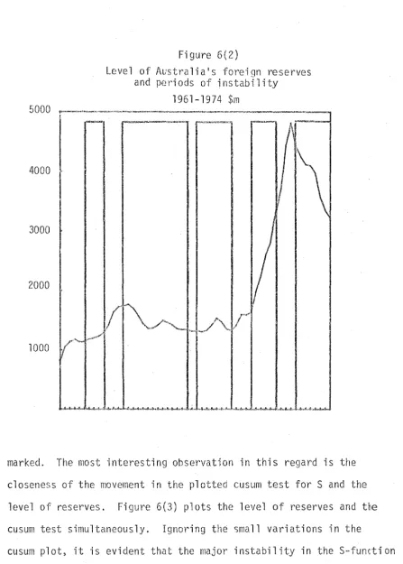
Much of the observed instability is obviously due to the changing weights on the targets during different phases of monetary policy. The SRD function is analysed in terms of the movement in Australia1_{s economic cycle.}

It is observed that there is a close connection between the per·iods of instability in the function and movements in the cycle. A similar analysis is carried out for the securities function, this time in terms of the movement in the level of foreign reserves. In this case, however, the connection is no as obvious or specific. The results of this analysis are presented in

Chapter 6.

involves an examination of several problems. The first focuses on the centra 1 issue of the authorities' philosophy towards monetary policy: either they set the ·instruments endogenously and in response to move-ments in the policy targets, or they set the instrumove-ments independently. If the instrument setting is endogenous, then a number of related issues arise. The first is found in a comparison of the response of the

individual instruments. A differing response in each case may indicate that the authorities have assigned the instruments to deal with specif:c economic problems. A second related problem concerns the potential interdependencies that may exist between the instruments themselves. A leading example is the nature of the relationship between interest rates and the success of open market operations. A final issue is the temporal stability of the policy responses.

working knowledge of the behaviour of the instruments required to control the money supply. This thesis attempts some preliminary_work in this direction.

1 . 1

tl~th..Q90

1.~-The genesis of this thesis is contained in a detailed review of the monetary literature. This review is presented in two related parts. The first focuses on the relevant aspects of the monetary-fiscal debate which brings to light two fundamental issues: reverse causation

and the iden-tification problem. The reverse causation argument centres on the issue of whether the money stock is the cause or effect of economic activity. If it is the cause, then changes in the supply of money

influence the level of economic activity. The alternative view is that changes in the money stock are engendered by changes in the level of activity. In brief, the fanner view treats the money supply as an exogenous variable whereas the latter treats it endogenously. Much of the criticism contained in the monetarist-fiscal debate concerns the definition of the key aggrega·tes. There is clearly an impor'tant identificat1on problem. The success of the empirical tests, which support one or other of the views, depends upon the way in which the

variables are defined and identified. Thus the first step in this dissertation is to draw out the relevant issues in the monetary-fiscal debate on these two basic issues.

Given the importance of the endogeneity problem and reverse causation, it is necessary to review the literature relating to these problems. Endogeneity of the instruments of monetai~y policy is

function for each instrument. These functions explain the instrument setting in terms of the targets of economic policy. The incorporation of reaction functions in structural models of an economy clearly affect the size of the dynamic policy multipliers. The review of previous reaction function studies provides insigh~s into the identification problem mentioned earlier. Each study has attempted to define the variables in the most suitable way. Clearly~ none of the earlier formulat·ions are suited exactly to the present problem, although they provide valuable background.

The identification problem is resumed when appropriate reaction functions are formulated for the Australian monetary policy instruments. Here, three policy instruments are defined: the SRD r'atio, the Reserve Bank1

s holdings of Government securities (S) and 1

the' interest rate. The first two are treated endogenously and reaction functions are

formula ted for them. Reasons are advanced for treating the interest rate as an exogenous variable in the equations for SRD and S. These two

reaction functions embody three short term policy targets: the rate of inflation (~),the rate of unemployment (U) and an external target (FR). In addit·ion~ the equations are formulated to accommodate interdependencies between S and SRD.

periods of instability. The th~sis concludes with a summary of the policy implications of these reaction function studies.

1.2 Scope

The study is confined to the time series 1961(1) - 1974(4). Quarterly data is used throughout the analysis in preference to both monthly or annual data. Monthly data is not available for all the variables used in the analysis. Quarterly data is more appropriate for the current study than annual data because the test concerns the short term reaction of monetary instrurnents to targets. There may be a current period reaction within the month but this is ignored because of the lack or unreliability of monthly data. The study focuses on the within ~uarter reaction.

The thesis concentrates on an evaluation of monetary pol 1cy reaction. Government expenditure functions are estimated but prove to be relatively insignificant. Government expenditure is found to respond primarily to growth. Also, the quarterly time period is obviously too short for this fiscal instrument, which is more realistically seen as a longer-run policy variable. Within the context of a quarterly model, therefore, it appears more appropriate to assume that government

expenditure is exogenous. The instruments of fiscal policy are more likely to be endogenous within the context of a model fitted to annual data.

The estimates of the two reaction equations are based on

series considered.

1.3 Outline of thesis

Chapter 2 contains the first part of the review of the literature. This draws out the relevant aspects of the monetarist-fiscal debate. In particular, the two issues of reverse causation and the identification problem are emphasized. The second aspect of the review of the literature is contained in the third chapter. There, the problem of endogeneity is discussed in general terms and the various reaction function studies, evoked by this issue, are analysed.

Reaction functions for Australia are specified in Chapter 4. Two equations are formulated, one for the SRD ratio and the other for the Reserve Bank•s holdings of Government securities. These instruments are preferred to the cash base or the money supply since they both have their impact on the money supply in different ways. This point is

illustrate~ by reference to a simple model of money supply dftermination. Chapter 5 presents the results of the reaction function estimation.

CHAPTER 2: TWO APPROACHES TO THE STUDY

OF THE IMPACT OF MONEY AND MONETARY POLICY

---·---~~·---"~

~-·----The monetarist-fiscal policy debate has proceeded unabated for a number of years. The extremities i~ the debate are concerned with the relative effectiveness of monetary policy action in influencing the economic aggregates. At one extreme are some Keynesian economists who argue that 1

money does not matter at all'. At the other extreme are those monetarists who sponsor the view that •money matters most•. The resolution of the controversy depends upon a detailed empirical evaluation of the issues involved, and although fue monetarists would claim that past empirical work strongly supports their position, the results are far from conclusive.

This present chapter concerttrates on a review of the 'monetarist' approach and, in particular, recognizes that such an approach has proceeded along two lines; the direct estimation and the structural model approach. Both will be reviewed in this chapter. The major emphasis in this chapter is on monetary policy, which is the suoject matter of this thes·is. t~onetary and fiscal policy however, are closely linked, and we cannot avoid comparisons of their relative impact and effectiveness.

Several important points are necessary before a revimv of the 'monetarist' approach can be undertaken. The points Y'elate basically to the inaccuracy of postulating a strict 'Keynesian' approach in which money is held to be unimportant. In fact, the two protagonists in the

activity. Whereas the extreme •monetarist' view that 'money matters most• is taken to preclude the influence or importance of fiscal policy, the opposite argument does not hold. Keynesian theory has always recognized the importance of both monetary and fiscal policy

on econom·lc .;.ggregates. Leijonhufud' s [33] re-appraisal of the Keynesian revolution is one major attempt to draw the important distinction between Keynesian econorrzics and the economics of Keynes.

In doing so, the author assigns a far more important role to Keynesian monetary policy, especially in the maintenance of full employment.

The genesis of the 'monetary-fiscal' debate occurred with the publication of the study by Friedman and ~1eiselman [20] (hereafter referred to as F-M) in which the authors sought to compare a quantity theory mode1 and an autonomous expendituh~ ('Keynesian') model of induced changes in the economy. This study repr'esents the starting point for the so-called 'direct estimation• approach to the monetary-fiscal debate. The F-M study is subject to considerable criticism and in the aftennath Andersen and Jordan [6] (hereafter referred to as A-J) attempt to modify and extend ·the F-·M results. This study also is

reviewed in detail.

These single-equation studies are then compared with studies

fact that the author emphasizes his preference for experimenting with monetary policy. Two ·important observations are made on the alternative approaches to the study of the monetary-fiscal debate: firstly, neither the direct estimation nor the structural equation models accommodate the potentia·; endogeneity of the policy ·instruments; secondly, they both fail to adequately define the instruments of monetary policy. These tv10 associated problems serve to provide an introduction to the so-called

'reaction function' studies and the general problem of endogeneity, both of which are discussed in Chapter 3.

2.1 The Friedman-Meisel!:nan_,_st!:!iY_

The first major development in the exposition of the monetarist view comes ~t.'ith the publication of the study by Friedman and Meiselman. Th·is study seeks to compare a simple quantity theory mode'! vrith a simp'le autonomous expenditure theory model. F-M maintain that the important argument in the debate is not theoretical but empirical. In terms of this empirical approach, the two theories compared by F-M conflict as to which of the two relationships is:

(i) critical in the sense of being the primary source o7 change or disturbance in economic activity;

(ii) stable, in the sense of being able to express, empirically, a consistant relationship.

Y

=

a +

V'M

( 2. 1)

Y

=

a+

K'A

(2.2)

where y

₌

_{nominal commun·ity income} M -· sr.ock of money

v·

=

income velocity

A

-·

autonomous expenditure

K'

=

marginal autonomous expenditure multiplier.

The criteria for choosing the periods of time to be studied

are firstly, that the comparisons be made for relatively short periods of time, and secondly, since the relationships might differ at different phases of the economic cycle, it is necessary to ensure that one

comparison covers one or more complete cycles. This will avoid any source of distortion from cyclical variations. The authors select the period 1897-1959. Annual observations are used for the entire period, but quarterly observations are introduced from 1945 onwards. The tim2 period is broken into thirteen sets of subperiods for which annual data is used, and one or two subperiods for ~tlhich quarterly data is used. These various subperiods are as follows:

Annua]_ly Quarter_l,t

1897 - 1958 1945(3) - 1958(4)

1897 - 1908 1946(1) - 1959(4)

F-M also encounter a statistical problem brought about by the correlatior. between the variables on the two sides of the equation (2.2). Since, by definition,

Y

=

C + A (2.3)

then observations of

Y

and

A

for the same period would entail correlation of

Y

with some part of itself. Thus, the authors argue that it is

preferable, in the absence of lagged responses, to use

C

=

a+KA

where C

=

induced consumption expenditure and K

=

K' - 1.

Equation (2.1) is correspondingly altered to

C

=

a +

VM

The authors also combine (2.4) and (2.5) to obtain

C

=

a + KA +

VM

(2.4)

(2.5)

(2.6)

This particular formulation is estimated in order to determ~ne

whether the correlation between C and M is significantly different from the correlation between M and A. The partial correlations of M and A indicate the net contribution of each to the explanation of C, keeping the other constant.

Price indices are also added as an additional independent variable, resulting in the following equations:

C

=

a +

VM

+ BP

C

=

a + KA + BP

C - a +

VM

+ KA +

BP

(2.7)

(2.8)

One important implication of using these real variables is pointed out by the authors. They suggest that when nominal magnitudes are used, it is plausible to suggest that the direction of causation would run from the stock of money to the dependent variable (CorY).

In the cas~ of real variables, however, the direction of causation is not as clear cut, since the money stock (real) is not under the control of the monetary authority as is the nominal value of the money stock. This is because the public determine the real stock of money by bidding prices either up or down.

Apart from the basic criticisms of the

F-M

approach (see

2.1.1

below), Stephanie Edge [19] suggests that the form of the equations used by the authors is not well founded theoretically. She suggests that, out of the six equations tested, only two

[(2.8)

and

(2.6)]

can be

legitimately derived from theoretical models. Rao [43], in a matl.c;matical exposition of the problem, attempts to show that such a criticism cannot be substantiated, and that the six equations tested can be grouped

according to whether or not they assume the existence of 'money illusion•. In attempting to define the variables to be used,

F-M

fin~ that there is no clear-cut agreement on the statistical definitions of

•au~onomous' and 'induced' expenditure, and no criteria for choosing particular definitions. This aspect of the monetary debate forms the subject of numerous articles which followed publication of the

F-M

study. Its importance is critical however, since many analysts suggest quite correctly, that the

F-M

findings stand or fall on the accuracy, or

th . f th . d f. . t. l o e rw 1 s e , o · ·- e 1 r e 1 n 1 1 on s .

1. The definitions eventually decided on were:

M

=

currency in public circulation+ adjusted demand deposits + time deposits in commercial banks

A

=

net private domestic investment + government deficit on income and product account + net foreign balance

Describing the results of their findings as •remarkably consistent and unambiguous' and the evidence obtained as 'one-sided•, F-M find that, for the 62 years as a whole, and for al~ but one of the 12 overlapping periods, and for both annual and quarterly data (after

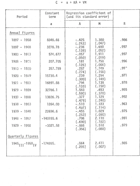
1946)9 the stock of money is more highly ~arrelated with C than is the level of autonomous expenditures. The only exception to this result is the period 1929-39 in which autonomous expenditures are found to have more influence on consumption than the money stock. Table 2.1 below tabulates the results of estimating equation 2.6.

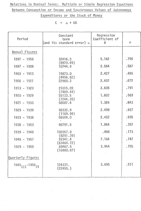
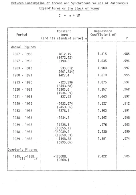
Tables 2.II and 2.III below tabulate the regression equations 2.4 and 2.5 for the various overlapping periods, as-well as the quarterly regression from 1945 - 1958.

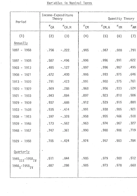
The results obtained also support the view that a positive correlation between C and one of the other variables might simply reflect the influence of this other variable in disguise. The partial

correlations show that except for the period 1929-39 the relation between A and C is simply a disguised reflection of the effect of M. The positive correlation between M and A produces a simple positive correlation between A and C. The authors find that, when M is held constant, the partial correlation between A and C is small and often negative. However, the partial correlation between M and C is almost as strong as the simple correlation coefficient except for the period 1929-39. See Table 2.IV below.

The introduction of the price variable in the equations emphasises the •one~sided• nature of the results. For every period except 1938-53, rCM.P > rCA.P' and, in this particular period, both

TABLE 2.1 Relations in Nominal Terms:

B~tw~_n. ___ y_9__!:!~U_II!Qt ion or Income 9_nd -~ynchronous Values of Autonomous

1~~nditures or

tpe

Sto~~-~fJ~oney

C

=

a +

KA

+

VM

·----·--··-~--·--·- ·

-R~;ression

coefficient of

~---··l

Constant

Period term (and its standard error)

a A M R

·--··-.---~---

- - - -

---

-!\nnua 1 F" . l res

1897 - 1958 8348.66 -.425 _. l. 380 .986

\

t.243, (. 047)

1897 - 1908 3278.78 -·. 238 1. 690 .997

( . 139) (. 052)

1903 - 1913 574-.677 -.057 1 . 911 .997

( . 050) ( . 019)

1908 .. 1921 207.705 . 181 l. 750 ,996

( . 126) (. 064-)

1913 - 1920 357.789 .287 1. 74-9 .99"

( . 27 4) ( . 158)

1920 - 19i9 15730.4 .239 "1. 294 .971

(. 300) (. 149)

1921 - 1933 16891.88 .794 1.138 .978

( . 133) ( . 1 50)

1929 - 1939 32786. 1 1. 583 .653 .955

( . 590) ( . 370)

1933 - 1938 13826.75 .377 1.129 .992

(. 479) (.240)

1938 - 1953 1264.00 -.510 1. 333 .963

(. 407) ( .114)

1939 - l 948 22696.6 -.455 1. 029 . 975

(.253) (. 090)

1948 - 1957 -140155.6 .706 2.110 . 991

(.690) ( . 182)

1929 - 1958 -3321.58 -.866 1. 518 .979

(.356) (. 088)

_Qua_Tterl_y _ _l_i__g_~re~

1945II C 1958IV -174895. .064 2.411 .985

l (

.205) (. 007)

--- -·-...

[image:17.556.47.531.182.823.2]

---I

I

TABLE 2.II

.R~C1 t i 0.!1 s i n _N._o_!!!_f.Q~_I~_r!!l~U l _ _!.iEl_~_o Y' Simp 1 e:__8~e s s i o l:!__l_q~_a t

i.

on~­

!?~t \Ale ~!.!... .. ~9l}~..!:!i!]F_"tj.Q!2__.2!_) nc O!!le a Q_Q__~yn c h ron o u_s_\{_~~ e ~£. ~_!on Q_~o u s

~d1J:ure~. or __ t_be S!!?_ck of Mon~y

C:.::: a+KA

-.~

Constant Regression

Period term Coefficient of

its standard error) a A

Jjn n~_a

1.-fJ.uu

res

1897 - 1958 32416.3 5.162 .756

(8970.45)

1897 - 1908 10744.9 2.564 .587

1903 - 1913 15873.0 2.427 .485

(4456.62)

, ( ) ( ) 0

1921 22968.3 2.407 .672

.

1:7VO - _I

I

1913 - 1920 21015.09 2.606 . 791

(7489.44)

1920 - 1929 55133.5 1. 602 . 569

(7244.35)

1921 - 1933 58587.4 1.384 .843

1929- 1939 58335.9 2.498 .937

(1169.94)

1933 - 1938 56504.0 2.452 .935

.

1938 -· 1953 96791.5 1.864 .397

1939 - 1948 102057.8 .494 . 173

(8291 .39)

I

1948 - 1957 26341.4 7.164 .747

(63464.72)

I

1929 - 1958 68467.5 3.944 .705

(16980.87)

Q'=! a r· t e_rJ_y_ll_g~~r e s

l

l945II I-1958IV 124331. 3.695 . 511

[image:18.554.46.523.112.822.2]

TABLE 2.III

Re l~!.ig~_llllomLnaj_Ierms~_ .. Mu_l!]2l_e or Simp 1 e Regc_~_ss i oQ__J_9.!:!_~ti o_Q_~

~£Ltl:i~f:?_Q_ __ ~_Q n S!JI~I?..t. i o_~g_r:_J..!_!f.._Orn~-~~~.z!.l.f_h r_o no u s_'Jjl ·1 u e~_f __ f\u ton omou_?_

~xpen.di !.l:!_r~~~he Stgc~Q.i ~~o~~

C == a + VM

---·---·

Period term Coefficient of

(and its standa rei error) a M r

---Con~ta~~----·-J Regression

-1---·---·-·-t- ·--··--·-- - - - · - - - · · - - - ·

-1897 - 1958 1897 - 1908 1903 - 1913

1908- 1921 1913- 1920 1920 - 1929

1921 - 1933 1929 - 1939 1933 - 1938 1938 - 1953 1939 - l9l~8 1948- 1957 1929 .. 1958

[Qua rJ:~ r lL£l.9_ll_re s ' 7812.15 (2472.42) 3190.3 533.612 ( 601.234) 1427.4 -123.296 (2443.68) 15303. 6

(4934.39) 337.53 -9432.974 (9453.36) •7278. 6 -2434.5 17438.1 (l 0055. 7) -140039.6

('18659. 53) -1198.28 (6995.66) 1 1. 315 1. 635 1.900 1. 810 1. 875 1. 357 1. 663 l. 527 l. 303 1. 262 .976 2.230 l. 351

.985 .996 .997 .995 . 991 .968 . 897 . 912 . 991 .958 . 963 .990 .974

"194 5 II I- 1 958 I

v '--··---_,_

7_5_0._88_. _____________ ,J..._ _ _ _ 2_. _4_2_2 _____ - . J . _ _ . 9.85

I

[image:19.559.49.525.137.820.2]

TABLE 2.IV

_Cj:>_!'re 1 at ion:;_ Bt::~ween _j_yn chron<;>us Vadabl in Nominal Terms

r

---

Income--Expenditure

Theory

Period - - +

~~---~:: --~;:;M

I

AIJ.Q.Ua lly

1897 .. 1958

1897 - 1908 1903 - 1913 1908 - 1921 1913 -· 1920 1920- 1929 1921 - 1933 1929- 1939 1933 - 1938 1938 - 1953 1939 - 1948

1948 -· 1957

1929 - 1958

Q\}.9 r!.~.dL

1945III-l958 1946!-19581 .756 .587 .485 . 672 . 791 -.222. -.496 -.127 .400 .423 . 569 . 288 . 843 .884 .937 .688 .935 . . 414

.397 -.328

.173 -.562 .747 .361

.705 -.4Z4

. 511 . 687 .044 .286 (4) .985 .996 .997 .995 . 991 .968 .897 . 912 . 991 .958 .963 .990 .974 .985 .985

Quantity Theory

(5) (6)

. 967 . 988

.996 .991

.996 .987 .993 .975 .980 .975 .956 .923 .529 .938 .955 .974 . 980 . 957 .979 .973 .933 .810 . 915 .985 .966 .967 .986 .983 . 980 .978

( 7)

I

I

. 791

I

.622 1

. 495

I

.6461

.761

I

. s24

I

I

.586 1

.880 1

.921

i

I

. sao

1

.327 1

. 719

.784

. 512 .660

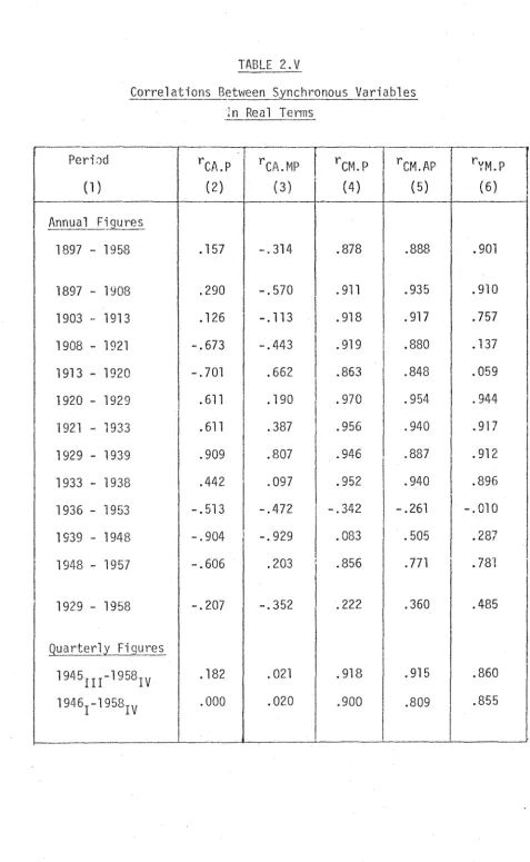
[image:20.556.39.522.134.824.2]

in Table 2.V below, also confirm the dominance of mon~y over autonomous expenditures. Holding both prices and autonomous expenditures constant,

money and consumption are, overall, more highly correlated than are autonomous expenditures and consumption when prices and money are held constant.

!n other experiments, the authors use quarterly data, in a seasonally adjusted form, to test for lagged relationships. They find, for example, that the simple correlation coefficient between C and M is highest when C is correlated with M two quarters earlier. See Table 2.VI below. The corresponding relationship between C and A is for the first quarter. In this case, the correlation becomes negative when the lead of A over C is extended beyond 4 quarters.

The authors carry this examination of the lagged relationship a step furtl1er·, and consider the effect of M and A on the subsequent behaviour of C, by computing the multiple correlation equations b~tween

C and the values of M and A in a successively larger number of quarters. The results, shown in Table 2.VII below, show that the multiple

correlation coefficient tends to rise only sligh~y when additional values of A are added, but tends to rise greatly as each additional value of M is added. According to F-M, these correlations provide evidence that the stock of money has an influence on later levels of consumption.

F-M also investignte further lagged effects by correlating C with pr·ior values of both MandA. From the results, given in

TABLE 2.V

- - - - ·

i;_orrelattons~etv.Jeen ~_ynchro!Jous _yariables l n Rea 1 Terms

...-·---r-·---··

Peri8d r _{r CJL\. MP}

rCM.~-l-

_{rCM.AP rYM.P}

1

CfJ. .• P

(1) (2) (3) (4) ( 5) (6)

1--·--

- -- -

-A n_n u a 1_ F 1.9..YX~-~

1897 - 1958 • 157 -.314 .878 .888 . 901

1897 - 1908 .290 I _{-.570 . 911 .935 .910}

1903 "' 1913 . 126 -.113 . 918 . 917 .75'7

1908 - 1921 -.673 -.443 .919 .880 . 137

1913 - 1920 -. 701 .662 .863 .848 .059

1920 - 1929 . 611 . 190 . 970 .954 .944

1921 - 1933 . 611 .387 .956 .940 .917

1929- 1939 .909 .807 .946 .887 . 912

1933 - 1938 .442 .097 .952 .940 .896

1936 - 1953 -.513 -.472 -.342 -.261 -. 010 1939 ·- 1948 -.904 I _{-.929 .083 .505 . 287}

1948- 1957 -.606 .203 .856 . 771 .78'1

1929 .. 1958 -.207 -.352 .222 .360 .485

Quarterly Fi9L!Ies

1945III-l958IV . 182 . 021 . 918 .915 .860

J

[image:22.557.46.523.45.820.2]

TABLE 2.VI Simple Con·elation Coefficients 3etvJeen Lagaed Variables 0· t l F. 'OLl5 -1058 '-~uar er y 1gures, 1 .... III 1_, .)IV

--i

-Dependent

!

Independent Quarters of Lead of Independent Variable Variable 1 Variable ' I . O l 2 3 4 5 6 7 8 9 10 , !

c

A

I

.

511 . 328 . 187 .074 -.005 -.088 .-.155 -.208 -.238 -.284 -.314.

l l

c

I

M

i

.

985 . 988 . 989 . 988 . 986 . 982 . 977 • 971 • 967 . 962 . 957

t~

I

c

II .985 .982 .979 .976 .974

y _{~c ~c}

~y r~ . 980 . 981 . 980 . 977 . 972 . 966 . 960 . 954 . 952 . 9tr7 • 944

!

I

.

---1---~A ~M ~r~

1-.

598 . 162 -. 173 -. 377 . 11 0 -. 342 . 258 -. 114 . 237 -. 032 -. 090

l

I

.

TABLE 2.VII Relations Involving Lagged Variables: Regression Equations Between Consumotion or Income and Va 1 ues of Autonomous Expenditures or the Stock of t·1one_y_~_j!l th~ Same and Earlier' Quarters, Quarterly Figures, 1945 111 -1958IV Constant Term { Regression Coeffi ~i e~t~~f-(and--its ~t~nd-at~de~;;;-;}-~ 1

I

~ep~nde~t

l

(and its

r

11 l t \ar,ablc

I

standard error)l At At-l nt_ 2 At_ 3 At_ 4 At-5

I

~

ct

ct

c ...

'-ct

ct

ct

I

124.33 13.695

I

.511

I

(22.455) (.863)

I

1 I ' 128.04 I 4.316 -.759 I .517 I (23.304)

I

(1.297) (1.178)

I

I

133 .. 01 I ,1_409 .337 -1.363. i .535 i (23.617)

I

(1.296) (1.507) (1.175)

l

I

137. 18

(24.163) 136.99 (25.520) 141.86 (26.073)

4.230 .559 -.521 -1.029 (1.315) (1.533) (1.528) (1. 189)

4.240 _(1.389) 4.421 _{( l} . 404)

.557

( l.

550) _.057

( 1.

404)

-.529 _{( 1.}

580)

-.506 _{( 1.}

641)

-1.054 (1.549) -.

727 ( l. 582) . 031 (1. 251) l. 026 (l. 589) -l. 200 (1.279)

I

,

1 . 545 1

I

.545

Table 2.VII continued Relations Involving Lagged Variables: Regression Equations Between Consumption or Income and Va 1 ues of Autonomous Expenditures or the Stock of Money, i~ th~ Same and Earl iet· Quarters, Quarterly Figures, 1945 111 -1958IV ! fConstant

Ter~

Regression Coefficient of (and its standard error)

I

I

I

Dependent

I

(and its , 1

I

Variable !standard error)!

i'\

Mt 1 M_,_ 2 l~t 3 Mt Ll. M .. r:: 1 R '! > ~ ~ V - L.- ._,--I ~v-..; f , ' ' I 11 1

c

I

-175.09 I 2.422

I

.985

I

t I ( 9. 668) ( . o59 1

l

I i .

·

ct

j -174.24 -.833 3.278

!

.988

l

'I· (8.772)

i

(.933) (.938)

I

I

1 ! ! l I

I

!

-171.32 II .859 -.874 2.45:)

!

.989 . , (8.5oo) (1.149) (1.986) (1.044) 1 I

I

I I ! I -166.92 !1.230 .229 -1.525 2.478 ! .990

I

' (8.329)

l

(1.109) (1.953) (1.936) (1.035)

I

I

ct

ct

Dependent Variab

1

e

c ..

"'

ct

ct

ct

TABLE 2. VII I Relations Involving Lagged Variables: Regression Equations Between Consumption or Income and Values of Autonomous Expenditures or the Stock o~· Money, in the Same and Earlier Quarters, Quarterly Figures. 1945

1

~

1

-1958IV (and its ' Constant. Term

I

Regression Coefficient of (and its standard error) 1 standard error). Mt At Mt-l At-l Mt_ 2 At_ 2

t\_

3 At_ 3 Mt_ 4 At_ 4

j

I 1 ' I • ; -174.89 I 2.411 .064 . 1 1 .985! ( 9. 772)

I

(.

07 0) (. 205) I l I -173. 23 1-1.112 . 263 3. 518 -. 036

l .

988 . (8.952) j(l.o29) (.26o) (1.o2n (.228) 1

I

'

'

I

The authors compute relationships between the first

differences of the variables, in an attempt to remove the effect of a common trend. The modified results tend to confirm the general

conclusions and although the correlation coefficients are low, they are largest whPn changes in C are correlated with changes in M in the

preceding quarter. No systematic pattern is found in the correlation between C and A, and both negative and zero correlation coefficients are encountered. These results are tabulated below in Table 2.IX.

The major implication of the F-M study is the conclusion that monetary policy is likely to be more predictableand to have a larger impact on income than autonomous expenditure. Some elaboration of this conclusion is necessary, especially in regard to the channels through which monetary policy has its ultimate effect on income. Again, the quantity theory and income-expenditur·e models ar·e at odJs.

In a Keynesian context, changes which occur in the money

stock are transmitted to aggregate income via changes in interest rates. These changes in interest rates which form the tr'ansi'tion mechan-ism,

affect the level of investment spending which, in turn, affects the income aggregates by way of the multiplier process. On the other ~~nd.

the quantity theory assumes that the public has some desired stock of money relative to its income. Any alte~ation to the stock of money

alters this desired ratio and induces a response by the public which vrill

be aimed at restoring the desired relationship.

It is this response which is the source of changes occurring in the level of income. In comparison with the Keynesian •credit' view therefot'e, the quantity theory approach suggests that changes in the stock of money operate through a whole range of expenditures rather

TABLE 2.IX Relations Involving Lagged Variables: Regression Equations Between First Differences of Consumption or Income and First Differences_of Values of AutonomlUS Expenditures or the Stock of Money for the Same and Earlier Quarters, Quarterly Figures, 1945 111 -1958IV ~~ -Constan~ Term-r Regression Coefficient of (and its standard error)

I

f

I

,

uependent (and 1 ts 1

!

I

I

variable standard error)

I

~;,At ~;,At-l ~;,At_

2

~;,At_

3

~;,At_

4

~;,At-S

!

R

I

. i

l

i;,Ct

I

21.079 I -.390.

I

.

598 :1: I

I

(1.486)

l

(.072) l I l

I

I 20.176

I

-.383 .039 I .601 I (2.288)

l

(.074) (.074)

-I

21.309 I -.377 .030 -.055 i .606 1 (2.779)

I

{.075) (.076) (.075) I 25.075 1 -.333 .o61 -.o96 -.22s 1 .6oo 1 (2.816) 1 (.o7o) (.o7o) (.o?o) (.o71) 1 1 25.729 \-.339 .067 -.090 -.230 -.034 I .692 _ ( 3. 164) 1 ( • 072) (. 072) (. 072) ( . 072) ( . 073)

I

! I !

I

27.602

I

-.326 .052 -.072 -.213 -.050 -.111 1 1 1 .709 ~~· 1

l

(3.352) [ (.o71) (.on) (.on) (.on) (.o73) (.o73)

I

I

1 r -1 ,

L

I I ' I

Table 2.IX continued Relations Involving Lagged Variables: Regression Equations Between First Differences of Consumption or Income and First Differences of Values of Autonomous Expenditures or the Stock of Money for the Same and Earlier Quarters. Quarterly Figures, 1945 111 -~958IV

lcons~ant

Term

l-R~re-ssion

Coefficient of (and its standard error)

I

-~

l

Dependent 1 (and its

l

1 1

I

Variable 1 standard error) 1 M\ 6~1t-l M\_ 2 M\_ 3

L~~\-4

6Mt-S

I

R 1 t I ,

-!

I

8Ct

I

ll . 193

I

.

889 II . 297 J

I

I

(1.057)

I

(.397) .

I

. ! I I ,

!

i:~Ct

I

l 0. 620

l

.

405 . 706 I . 359

I

1 (

1.,

on

I

(.

502) (. 457) I i:~C

I

10.695 ! .420 .777

I

t

I

(1.159)

I

(.510) (.546) I I • ! 6C

l

l 0. 590

I

.

409 . 694 1. t

l

(1.173)

~,·

(.513) (.560) ' I

l

l I 6Ct

l

10.567 I .382 .713 I 11 1 ( l. 190) ! (. 533) (. 573) I I ' l

l

i:~Ct

j 1 0. 4 94

I

.

420 . 650 I 1 (1.216) I (.s4s) (.602)

I

I 1 !

-.115 {.472) -.309 (.

545)

-.339 (.568) -.315 (.

577)

• 321 _(. 444) .267

(.

517) _. 194

(.

577)

.098 _(.469) .002 _(.539)

.192

(.513)

I

.360

I

I

l I

.373

I

i

.374

I

I

The F-M study supports the monetarist position; the results suggest that the monetary instruments are the more effective vehicle of pol-icy. They also suggest that the quantity theorists' view of the operation of monetary policy is to be preferred to the Keynesian 'credit' argument. Changes in the money supply wor·k direci:Zy on aggregate

expenditure and are not transmitted to expenditure through the interest rate.

The large number of articles which followed publication of the F-M results is proof of the immense interest evoked by this study. 2 In a survey of the criticisms and weaknesses of the F-M approach,

Stephanie Edge concludes that the overall result of the original and subsequent studies is to lead the authors and others, 1

into an eco,,omic cul-de-sac' [19, p. 68]. The major criticisms of the F-M approach relate to the various definitions of both money and autonomous

expenditures. In addition, there are criticisms of the inclusion or exclusion of particular time per·iods, a.nd the problems caused by the estimation procedure.

It is in the definition of the autonomous expenditure variable that many consider the F-t1 analysis to be weakest. The majority of the critics maintain that nearly all the components of F-M's definition of autonomous expenditure are, in fact, endogenous, and should be eliminated from the final definition. Perhaps the main reason for this criticism

is the statistical criteria used by F-M in determining the exogeneity, or otherwise, of the various components of autonomous expenditure [20, pp. 182-185]. Lewis [34] considers in detail the selection process used by F--111, and amongst others, Edge [19, pp. 65-67] suggests that the authors are not always consistent in applying their criteria.

In his comment on the F-M paper, Donald Hester [25] argues that F-M have represented the autonomous expenditure theory in an

unorthodox form which makes it very sensitive to statistical comparison. He maintains that the inclusion of the government deficit and the net foreign balance in A is not entirely correct, and that these two variables are not likely to be completely exogenous.

In an attempt to improve the definition of A, Hester employs a simple model which recognizes the dependence of taxes on income. This is done in order to alleviate the alleged weakness in F-M's definition which, Hester argues, ignores the fact that taxation is a function of income. From his model, Hester considers four measures of A:

-L ::: _{I +} G + _H

-

_M

-L' -· L + M + 0

Lt' --

L'

M

Lu' :::

L'

_E

where I - net private domestic investment

G

=

government expenditure on income and product account H

=

exports

M

=

imports

In computing correlation coefficients to test the new definitions for the period 1929-58, Hester finds that, with the exception of the 1929-39 period, the correlation between C and every proposed measure of A exceeds the corresponding correlation between C and F-M's definition of A. He also finds that the correlations between C and any of the proposed definitions of A do not differ from the correlations between C and t~ by more than 0.06 for the 30-year time period studied.

In reply to Hester's criticisms. F-M [21] criticise Hester's use of a limited time period. They maintain that, if the World War II years are excluded, almost half of Hester's test period is made up of the years 1929-39 which they originally considered to be a period substantially different from other period~.

Ando and Modigliani (hereafter referred to as A-M) [9] also attempt to call attention to a number of basic shortcomings in the F-M paper. Making use of a full scale set of definitional expressions and identities, A-M test a consumption-autonomous expenditure relationship once again using a drastically altered definition of autonomous

expenditure .. 3

The equation tested fit~ the data well, and the fitting of a correlation between C and the newly defined autonomous expenditure

3. Their definition comprises net investment in plant, equipment, and residential houses, total government purchases of goods and services, exports, the property tax portion of indirect business taxes, net investment paid to government, government transfer payments

(i.e. unemployment insurance benefits), subsidies less current surplus of government enterprises, less the excess of wage accruals over disbursement. This can be compared to F-M1

variable reduces the unexplained variance by 90 per cent when compared with the original F-M equation.

In another major attack on the F-M paper, de Prano and Mayer [17] (hereafter referred to as O-M) submit further alternative

definition:.: of A, us·ing different selection techniques from those used by F-M. They suggest that the definition of A used by F-M (consisting of the sum of fixed private domestic investment, government deficit on income and product account, and the net foreign balance) contain

endogenous elements. To show this, 0-M correlate the various components of F-M•s definition of A with C to show how the correlation coefficient falls as non-endogenous components are added. From this test, the authors conclude that three components - inventory investment, imports, and the government deficit or surplus - are, in fact, endogenous.

0-M suggest that the new definitions of A4 used, tend to perform much better than the definition used by F-M in their tests.

The other major definitional criticism of the F-M approach concerns their choice of M, the monetary variable. Ando and ~1odigliani

[9, p. 708], for example, suggest that, during the period tested by

F-M, the variable M used was at least partly induced, and thus positively correlated with the error term in the tested equation. These authors maintain that there are adequate gr'ounds for suggesting that the causal links from the money supply to money income are more complex than F-M's analysis suggests. The high correlations obtained by F-M for the

4. A as the sum of investment in producers• durable equipment, non-residential construction, residential construction, federal government expenditures on income and product account and exports. A as the above definition less capital consumption measures.

A as gross fixed private domestic investment.

monetary variable may actually overstate the strength of the causal mechanism from the money supply to the level of income. Because of this fact, A-M experiment vJith another monetary variab'1e, M*, which they define as the estimated maximum amount of money that could be created by the banking system on the basi:, of the monetary authorities' reserves, taking into account the reserve requirements and currency holding habits of this authority. This approach is based on the somewhat dubious assumption that the bank's reserves are autonomous. In fact, it has been suggested that because deficit financing serves to increase bank reserves, M* is related to A, and this definition of a new monetary variable does not improve the F-t~ approach greatly [19, p. 59].

Other studies which attempt to l~edefi ne the monetary variable also base their criticism of the F-M definition on the fact that such a variable may not be truly autonomous. The studies by Barrett and

Walters [12] and Laumas and Laumas [31] highlight the fact that critics of the F-M approach recognize the problem of exogeneity in the definition of the monetary variable. Barrett and Walters 2xamine the possibility of a lag existing in the effect of money on consumption. Such an analysis is pursued with the aid of Friedman's 'permanent income' hypo~hesis.

Despite their exhaustive study, the authors are unable to conclude that

onl,y money or only autonomous expenditures are the predominant variable

i1:1portance of M and A, despite a detailed monetary analysis aimed at improving the F-M definition. The basis of this particular approach is a test of the so--called 'degree of moneyness' of va\'ious monetary definitions [30]. This approach merely leads to the conclusion that both A and the newly defined M are equally important in determining income, and that their relative importance depends upon the period considered.

The use of time periods differing in length is also the individual subject of debate en the Friedman-Meiselman paper. The authors themselves consider the entire period from 1897 to 1958, but ignore many of the results of the Depression years because they do not accord with their overall results and because they consider the period to be one characterized by breakdowns in the banking and financial system which wou·ld adversely affect the monetary mechanisms. In this regard, i t is worthwhile noting that the inclusion of the War years in the Friedman-Meiselman study has no detrimental effects on the obviously overwhelming superiority of the quantity theory in determining economic activity. Many of the critics of F-M's selected time period criticise the inclusion of the war years which bias the results in favour of the monetarist case because war time rationing produces a spasmodic pattern of consumption.

Other antagonists of the F-M approach also attack the

than conclusive. Other ctitics of the F-M approach are also less than conclusive in their attempts to solve this problem.5

One further criticism of the F-M approach st2ms from the author's use of a simple one-equation model to test the competing theories. P1ndo and fv1odigliani [9~ pp. 71L:·-16] are among the critics who question the meaning and relevance of simply comparing the

correlation coefficients for the variables A and M. They suggest that the F-M approach fails to shed any light on the problem of how the dependent variable, either C or Y, can be effectively controlled.

This faibre stems from two fundamental flaws in the F-M approach which have, as their basis, the use of the simple single equation model.

Firstly, A-M argue that there is no justification for the treatment of the autonomous expenditure variable and the money supply variable as mutually exclusive stabilization devices. In fact it is more accurate to suggest that the quantity theory is a theory of demand for money and, as such, is an important part of the Keynesian framework

of income determination.

Secondly, and more importantly in the context of the following chapter of this thesis, A-M suggest thut neither of the two rival

theories tested can be properly regarded as a behavioural or structural relation. Even if the independent variables used in the tested equations can be regarded as truly exogenous, at best they can be regarded as

'grossly misspecified "reduced forrns'11

[9, p. 715]. A-M,however, fail to agree that the independent variables can be regarded as truly exogenous.

At best, they argue, the independent var·iables can be regarded as

1

autonomous 1

in the sense of being uncorre l a ted with the erTO¥' term of the test equation. Such a situation is quite different from being exogenous in the economic sense. This particular problem, along with several othe:·s inherent in the F-M approach,also appear in the later monetary-fiscal studies of Andersen and Jordan [6]. The first article which appears to fully recognize the consequences of incorrectly

treating endogenous variables as exogenous is the study by Goldfeld and Blinder [23] who analyse closely many of the erroneous conclusions which may be reached under these circumstances. The general problem of endogeneity and the points raised by Goldfeld and Blindet· are discussed in Chapter 3.

2. 2 I!:!_~nd~[s_~rc~orq~_!]_-~tudy

The study by Andersen and Jordan (hereafter referred to as A-J) represents a step forward in the monetarist argument.

The basic thrust of the A-J approach is to place more emphasis on the relative attributes of monetary and fiscal policy, rather than merely atte~pting to examine the relative influences of money and autonomous expenditures in influencing income movements. Their study sets out to examine whether or not the response of economic activity to fiscal actions is (i) greater in effect; (ii) more predictable and

(iii) induces a more rapid response, than the response to monetary policy. They do not experiment with structural forms. For example, they_do not test for the directness or indirectness of monetary actions upon the aggregates.

author's; the monetary base and the money stock. The monetary base, which is assumed to be under the din;ct control of the monetary authorities, is defined to include reserve deposits of member banks at the Reserve Bank and all currency held by commercial or non-banks, adjusted for changes in r0serve requirements. Anders~n and Jordan, in an earlier article [7] examine the concept of the monetary base ~in more detail. They consider the base to be a good measure of monetary influence for

two reasons. Firstly, it acts as an important link between monetary authority actions and their impact on economic activity, and secondly,

it is considered to be a variable over which the monetary authorities have the most complete control.

The two monetary measures are chosen because of their strategic importance ·in both the Keynesian and the Quantity theory approaches to explaining movements in economic activity. The channels through which the tvJo schools view the influence of monetary policy have been exanrlned

6

previously in relation to the stock of money. The use of the monetary base simply adds a further stage of influence in that changes in the monetary base engender changes in the money stock which, in turn, affect prices, interest rates and spending in general over a wide range of capital and consumer goods.

Turning to a measure of fiscal influence, A-J suggest the use of so-called 'high employment' budget concepts. These comprise both expenditures (goods and services and transfer payments) and receipts

(legislated changes in Federal Government tax rates) which are adjusted for the influence of economic activity. The full employment budget

surplus (receipts less expenditures) is also used. To test the

empirical relationships, quarter-to-quarter changes in GNP are regressed

on quarter to quarter changes in the money stock and the various measures of f·i seal policy. The various equations tested are as follows:

t,GNPt ::: _{ao +}

a1M\-n + a₂6(R E)t-n (2.10)

t,GNPt ·- _bo + blt,Mt-n + b2AEt-n + b36Rt-n (2.11)

t,GNPt

-

c +

c-1 AMt-·n + c26Et-n

0 (2.12)

(2. i3)

where GNP

=

Gross National Product at constant prices

t•1 :::: money stock

R :::; high employment Government receipts

E :::: high employment Government expend _i tur·e

B

=

monetary base and n

=

1, 2 and 3 periods.

The changes in the variables are calculated using conventional •first differences• by subtracting the value from the previous quarter from the value for the present quarter. An averaging procedure known as

'central differences• is also used. This method necessitates the summation of the forward difference and the backward difference which, according to Kareken and Solow [26], gives a better approximation of a smooth rate of change at any point of time. The above equations [(2.10) to (2. 13)] are therefore estimated for variables calculated by both the normal •first differences• and the •central differences' methods.

necess ·i tates the a priori imposition of the 1 ag 1 ength, even though the actual lag structure is determined by the regression itself, rather than being imposed a prior'i.

In terms of the R2 statistic (adjusted for degrees of freedom) the results obtained fit well. The authors find that the estimated coefficients for both the money stock and the monetary base are highly significant and of the correct sign, whereas the estimated coefficients for the high employment measures of fiscal performance are not

significant and tend to vary in sign. The rAesults, using f·lrst difference and central difference techniques,are tabulated below in Table 2.X.

The monetary measures of either the money stock or the

monetary base perform extremely well, and are highly significant ove1A the four quarter lag distributi~n. On the other hand, as the table above displays, all measures of fiscal action fail to generate significa11t results. In fact, in the case of high employment expenditures, it is shown that an increase in Government expenditure is mildly stimulative in the quarter in which the increase occurs, but becomes negative in the

second and third quarters.

TABLE

2.X

Regression of Changes in GNP on Changes in Monetary and Fiscal Actions First (Eguation 2. 10) (~quation 2.11) (Equation 2.12) (Equation 2.13) Differences LIM LI(R-E) Ll~l LIE LIR M·1 L\E LIB LIE LIR - --t 1. 57* -. 15 1. 51* .36 . 16 l. 54* .40 l. 02 r.r-. . 52 .C) (2. 17) (. 65) (2.03) (1.15) ( ~""?\ \•J.Jj (2.4-7) (1.48) (. 49) (. 67) ( 1. 68) + ~ ~..-I 1. 94* -.20 l. 59* .53* -. 01 1. 56*

.... Ll* _.::>'

TABLE 2.X (Continued) Central (Equation 2. 10) (Equation 2.11) (Equation :2.12) (Eouation 2.13) Differences ~(R-E) ~M ~E ~R ~M ~E ~B ~E -.... 1. 50 -.24 l. 58* .53 .32 1. 54* .63* . 61 .28 1.. (1. 84) (. 91) (;:.ol) ( l. 52) ( 1. 05) (2.45) (:2_21) {. 28) (. 73) t-1 2. 11* -.23 l. 57* .60 -. OLl 1. 63* .59* h. 1-: ;;~ ...: • -r ~-.50 (3. 61) (1.16) (2.78) (2.44) (. 17) (3.57) (:2.61) (3.16) (1.87) t-2 1. 89* . 15 1. 41 * -.15 -.11 l. 43* ·-. 16 6.87* -.27 (3.18) (. 81) {2.45) (.60) ( .47) (3.16) (. 71 ) (3.92) ( l. 04) t-3 l. 06 .52 1. 26 -.96* . 18 l.l3 ·-.86* 3. 51 -1.26* ( l. 36) ( l. 90) (l. 72) (3.15) (. 48) { 1 . 71 ) ( 3. 07) (1.71)

('"'

h_,

.).L.!::l; Sum 6.56* . 21 5.80* . 02 .34 5.74* . 19 16.41* -.75 (8.16) (. 47) (7. 57) (. 04) (.54) (8.45) (. 77) (6.95) ( l . 37) Constant 2.02* 2.00* 2.30* 1.24 (2.48) (2. 14) (3.55) (1.14) R2 .66 .72 .73 • 67 S.E. 3.35 3.03 2.97 3.26 D-t~ .88 l. 14 1.13 l. 05 Note: Regression coefficients are the top figures, and their 't' values appear below each coefficient enclosed by parentheses.

~R .87*

(2.55) -.07 (.

27)

-.33 _(1.31) .35 (. 87) _.82

TABLE 2.XI Measurements of the Relative Importance of Monetary and Fiscal Actions First Differences (Equations 2.11 and 2.13) Beta Coefficients Partial Coefficients of Determination Quarter liM liE liR ! liB liE 6.R liM t,E liR I t,B liE liR I I -r ... .24 . 14 .05 .06 . 09 . 16 .07 . 02 . 01 I i: . 01 .05 l,

I l

above, for the monetnry variables, and the fiscal expenditure and receipts variables~

The results above indicate quite conclusively that changes in the money variables generally have a greater impact on GNP than changes in the fiscal high employment variables for the current period and the two quarters preceding the change. In those cases where ~E

provide the greater beta coefficient, it is associated with a negative coefffci ent sign, i ndi cati ng a contracti onary effect.

Pc. rti a 1 coefficients

U

-.c~ _ ... e~...., ... ..:-. ... .:-.,...7 a~r'lo ••rrtd

Ut:l- !llllllUl.IVII I t : U.:>t:: to check the

results for this proposition, and thes~ tend to coincide with the former results. See Table 2.XI. From these tests, the authors are unable to confirm the first proposition that fiscal actions are stronger than monetary actions.

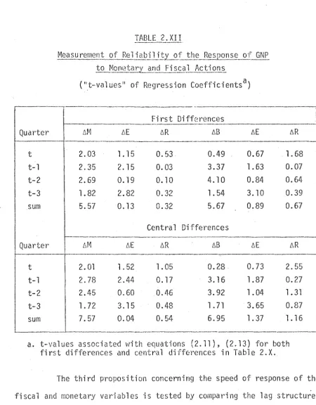
The second proposition, that the response of economic accivity

to fiscal actions is more predictable than the response to monetary influences, is tested by a comparison of the t-values (the value of the regression coefficient relative to its standard error) . . The higher the value of the t-ratio, the greater the reliability of the estimated change in GNP resulting from a change in the variable.

The two monetary variables outperform the fiscal high

expenditure variables in all quarters, except the third. See Table 2.XII below. The t-values for the sum of the regression coefficients are

extremely large for both ~M and ~B, but are not statistically significant for the 6E variable. Accordingly, the second proposition is not

confirmed.

TABLE 2.XII

Mea su rem~~~~-2.LB.~ l_i a b iJ_j_tL.Q_f the Res .1?.Q!:!. se __ ot_QNP

to_ Mo n (~ t~r,L..9.~~Q_J i _?.s:_~J....j-._c t i on~

("t-va'lues11

of Regression Coefficientsa)

·---·--~-~~~·-·-..-.~---·---·- ··---·----·---~

First Differences

- - - 1

Quarter !1M L1E L1R !18 AE AR

- - - ---~·--~3·~_... _ _ _ _ _ _

t 2.03 l. 15 0.53 0.49 0.67 l. 68

t-1 2.35 2.15 0.03 3.37 l. 63 0.07

t-2 2.69 0.19 0. l 0 4.10 0.84 0.

64-t-3 1.82 2.82 0.32 1. 54 3.10 0.39

sum 5.57 0.13 0.32 5.67 0.89 0.67

Centra 1 Differences

Quarter LIM liE liR 68 liE AR

t 2. Ol 1. 52 1.05 0.28 0.73 2.55

t-1 2.78 2.44 0.17 3.16 1.87 0.27

t-2 2.45 0.60 0.46 3.92 l. 04 1. 31

t-3 1.72 3.15 0.48 l. 71 3.65 0.87

sum 7.57 0.04 0.54 6.95 l. 37 1.16

----·---

----·---a. t-values associated with equations (2.11), (2.13) for both first differences and central differences in Table 2.X.

The third proposition concerning the speed of response of the fiscal and monetar·y var·iables is tested by comparing the lag structure of the regressions primarily in terms of the size of the beta coefficients in the quarter of the change and the quarter following the change.

[image:45.556.54.504.49.625.2]

t

.40 .

. 20

-.20 '

-.40

t+l

t-1 t-·2

Equation 2.11

.40

.20

0

... 20

-.40

t+l t

.40

.20

0

-.20

_, .40

t+l t

Equation 2.13

t-1 t--2

Equation 2."11

t-1 t-2

t-3 t-4

two quarters and a change in E is greatest in only the third quarter. Accordingly, A-J were unable to confirm that the major impact of

fiscal policy on economic activity occurs within a shorter time period when compared with monetary policy.

In discussing the implications of the three propositions

tested in the study, the authors basically conclude that monetary actions play a highly prominent role in economic stabilization. Evidence tends to suggest that the money stock is an important indicator of the general thrust of stabilization actions, basically because any changes in this var·iable reflect the discr·etionary actions of the monetary authorities in their use of the major instruments of policy.

Two Australian studies which have adopted the A-J approach are those of Dewald and Kennedy [18] and Sheppard [44]. Dewald and Kennedy duplicate the A-J study for Australia and find support for both monetary and fiscal influences, especially when unlagged equations are analysed. Using the Almon lag technique and either M

1, M2 or M3 as the monetary variable, the authors find that the evidence overwhelmingly

supports the monetarist position.

Sheppard duplicates Argy•s [10] reduced form approach,

regressing annual percentage changes in GNP against annual percentage changes in M

1 and M2 for the period 1950-1972. He finds that, by

altering Argy's time period, he obtains results which again support the monetarist view. Sheppard then estimates regressions with quarterly percentage changes in nominal, real and nominal less real GNP against quarterly changes in M

money supply and GNP. He admit:; that there is a pass i bi 1 ity that some of this association may be due to a reverse causation from economic activity to money, although he also po·ints out that much of the

fluctuation in the monetary aggr·egates is the result of policy actions rather thar the result of a simple 1

accommodating1

policy.

Sheppard also duplicates the A-J approach using either M 1 or M

3 as the monetary indicator, and Commonwealth Government spending, full employment Government receipts and exports as the fiscal indicators. The period covered is 1959(4) - 1972(1). In all cases, the fiscal

indicators prove insignificant, whereas the money supply variable is highly significant.

2.2.1 Criti~l?.~~qf the A-J appl~oach_

In general, the A-J approach manages to accommodate many of the criticisms of the F-M study. They overcome the criticism of the time period and the problem of trends caused by F-M's use of levels for the variables by using post-war quarterly first differences of data. Also, they use 'high employment' fiscal variables, carefully choosing the components of each so as to do away \·lith the arbitrary endogenous-exogenous allocation which was roundly criticised in the F-M study. The same principles are applied to the choice of a monetary variable, where both the money stock and the monetary base are used. A-J attempt

to alleviate endogeneity in these variables by giving results of their estimations for both the money stock and the monetary base.

progress made, or concession gtanted by way of determining a truly exogenous monetary or fiscal variable. Gramlich suggests that the problem is quite intractable, since 'it depends (as far as monetary policy is concerned) on~ first, whether the Federal Reserve is really exogenous in its short-run response to movements in aggregate demand, and, secondly~ on how this exogeneity can best be represented'. [24, p. 512] In this respect Gramlich touches on a point which is central to the whole problem surrounding monetary policy and the tests of its effectiveness and impact. He po·ints out that the pr·oblem of endogeneity can only be important in those cases where the authorities are not

constrained by competing objectives and where their actions are an immediate response to stabilization needs.

Despite these obvious improvements on the F-M approach, the large number of articles which have followed the publication of thd A-J study emphasize the fact that the problems of testing monetary and fiscal policy strengths still exist. For example, in a comment on the A-J studyj Frank de Leeuw and John Kalchbrenner [16] make use of

alternative equations which, they suggest, appear to cast doubt on the

A-J results.