Image and Volume Segmentation by Water Flow

G. Bebis et al. (Eds.): ISVC 2007, Part II, LNCS 4842, pp. 62–74, 2007. © Springer-Verlag Berlin Heidelberg 2007

Xin U. Liu and Mark S. Nixon

ISIS group, School of ECS, University of Southampton, Southampton, UK

Abstract. A general framework for image segmentation is presented in this pa-per, based on the paradigm of water flow. The major water flow attributes like water pressure, surface tension and capillary force are defined in the context of force field generation and make the model adaptable to topological and geometrical changes. A flow-stopping image functional combining edge- and region-based forces is introduced to produce capability for both range and ac-curacy. The method is assessed qualitatively and quantitatively on synthetic and natural images. It is shown that the new approach can segment objects with complex shapes or weak-contrasted boundaries, and has good immunity to noise. The operator is also extended to 3-D, and is successfully applied to medical volume segmentation.

1 Introduction

Image segmentation is a fundamental task. For example, in retinal images, vessel structures can provide useful information like vessel width, tortuosity and abnormal branching which are helpful in medical diagnoses. However, natural images often comprise topologically and/or geometrically complex shapes, like the vessels. The complexity and variability of features, together with the image imperfections such as intensity inhomogeneities and imaging noise which cause the boundaries of considered features discontinuous or indistinct, make the task very challenging.

based on repeated sampling of the evolving contour on an affine grid. Geometric active contours [8, 9] have also been developed where the planar curve is represented as a level set of an appropriate 2-D surface. They work on a fixed grid and can automatically handle topological and geometrical changes. However, many methods solve only one problem whilst introducing new difficulties. Balloon models introduce an inflation force so that it can “pull” or “push” the curve to the target boundary, but the force cannot be too strong otherwise “weak” edges would be overwhelmed. Region-based energy can give a large basin of attraction and can converge even when explicit edges do not exist but it cannot yield as good localization of the contour near the boundaries as can edge-based methods. Level set methods can detect complex shapes well but also increase the complexity since a surface is evolved rather than a curve.

Instead of model-based methods, some proposed the morphological watershed based region growing techniques [10, 11]. The approach is based on the fact that smooth surfaces can be decomposed into hills and valleys by studying critical points and their gradient. Considering pixel properties (intensity or gradient) as elevation and then simulating rainfall on the landscape, rain water will flow from areas of high altitude along lines of steepest descent to arrive at some regional minimal height. The catch-ment basins are defined as the draining areas of its regional minima and their bounda-ries can then be used in object extraction. Though assuming water collection, the method does not use the features of water itself and focuses on the image’s geo-graphical features. The non-linearity arising from issues like finding steepest descent lines between two points makes the method complicated. Moreover, the region growing framework often yields irregular boundaries, over-segmentation and small holes.

Unlike the mathematical models introduced above, we propose a physical model focusing on water itself rather than the landscape of images. Water is chosen because features like fluidity and surface tension can lead to topological adaptability and geometrical flexibility, as well as contour smoothness. We completely redefined the basis of our previous water-flow based segmentation approaches [12, 13] by adopting the force filed theory which has been used in feature extractions [14]. The method shows decent segmentation performance in quantitative and qualitative assessments. Further, the nature of physical analogy makes the working principles and parameters easy and explicit to interpret. The 3D extension is also more natural and straightforward than mathematical models like T-surfaces [7].

2 Methodology

Water flow is a compromise between several factors: the position of the leading front of a water flow depends on pressure, surface tension, and adhesion (if any). There are some other natural properties like turbulence and viscosity, which are ignored here. Image edges and some other characteristics that can be used to distinguish objects are treated as the “walls” terminating the flow. The final static shape of the water should give the related object’s contour.

D

= A R⋅

v F (1)

where A is the cross-sectional area of the flowing water and is set to unity here. FD comprises the pressure, surface tension and adhesion. The flow is mainly driven by the pressure pointing outwards. The surface tension, which is the attractive force between water surface elements, can form a water film to bridge gaps in object boundaries. The adhesion, which is defined as the attractive force from image edges to water surface, can assist water in flowing inside narrow braches.

For the image analogy, one pixel in the image is considered to be one basic water element. An adaptive water source is assumed at the starting point(s) so that the water can keep flowing until stasis, where flow ceases. The image is now separated into dry and flooded areas by the water. Only elements at water contours are adjacent to dry regions, so only contour elements are of interest in the implementation.

The implementation of the flow process of one contour element is shown by the flowchart in figure 1. Applying same procedures to all the contour elements forms one complete flow iteration. As shown by figure 1, the flow process is separated into two stages – the acceleration stage and the flow stage. In the first stage, the considered element achieves an initial flow velocity determined by the driving force FD and re-sistance R. Then we examine the movements at possible flow directions pointing from the considered contour element toward adjacent dry points one by one. For the direction i, the component velocity scalar vi is calculated. If vi > 0, the process then progress to

the next stage, where the element is assumed to be flowing to the dry position related to the direction i and some image force is acting on it. To reconcile the flow velocity with the image force and hence conduct the movement decision processor, dynamical for-mulae are used. The movement decision is made according to the sign of J and

2

2 _i

i mv

J

F S

where S and m are defined as the fixed flow distance in one iterative step and the water element mass. In this equation, Fi is the scalar imageforce at direction i. It is defined to

be positive if consistent with i, and negative if opposite. J ≥ 0 means that the initial

kinetic energy exceeds the resistant work produced by Fi during S and thus the contour

element is able to flow the target position at direction i.

The definitions and calculations of the factors and parameters introduced above then need to be clarified. In this paper, the force field theory is embodied into the water flow model to define the flow driving force FD.

2.1 Force Field, Water Driving Force, and Flow Velocity

In this new water flow model, each water element is treated as a particle exhibiting attraction or repulsion to other ones, depending on whether or not it is on the contour / surface. The image pixels at the dry areas are considered as particles exhibiting attrac-tive forces to water contour elements. Now both the water elements and the dry area image pixels are assumed to be arrays of mutually attracted or repelled particles acting as the sources of Gaussian force fields. Gauss’s law is used as a generalization of the inverse square law which defines the gravitational and/or electrostatic force fields. Denoting the mass value of pixel with position vector rj as L(rj), we can define the total

attractive force at rj from other points within the area W as

D 3

,

( )

(

| |

) ( ) j k

j _k

j j k _{j k}

L − ∈ ≠ − = ∑ W r r r r

F r r (3)

Equation (3) can be directly adopted into the framework of the water flow model, provided the mass values of different kinds of elements are properly defined. Here the magnitude of a water element is set to 1, and that of a dry image pixel is set to be the edge strength at that point (an approximation of the probability that the considered pixel is an edge point). The mass values of water contour elements and image pixels should be set positive, and those of the interior water elements should be negative be-cause equation (3) is for attractive forces.

From equation (3), the flow velocity is inversely proportional to the resistance of water (the cross-sectional area A has been set to 1). In a physical model, the resistance is decided by the water viscosity, the flow channel and temperature etc. Since this is an image analogy which offers great freedom in selection of parameter definitions, we can relate the resistance definition to certain image attributes. For instance, in retina vessel detection, if the vessels have relatively low intensity, we can define the resistance to be proportional to the intensity of the pixel. Further, if we derive the resistance from the edge information, the process will become adaptive. That is, when the edge response is strong, resistance should be large and the flow velocity should be weakened. Thereby, even if the driving force set by users is too “strong”, the resistance will lower its in-fluence at edge positions. Thereby the problem in balloon models [2], where strong driving forces may overwhelm “weak” edges, can be suppressed. Therefore, such a definition is adopted here. The flow resistance R at arbitrary position (u, v) is defined as a function of the corresponding edge strength:

exp{ ( , )}

R= k⋅Eu v (4)

where E is the edge strength matrix and the positive parameter k controls the rate of fall of the exponential curve. If we assign a higher value to k, the resistance would be more sensitive to the edge strength, and a lower k will lead to less sensitivity. Substitute equations (3) and (4) to equation (1), the resultant flow velocity can be calculated. From figure 1, we can see that each possible flow direction is examined separately, so the component velocity at the considered direction, vi needs to be computed:

cos

i

v = ⋅v

γ

2.2 Image Forces

If vi ≤ 0, the contour element will not flow to the corresponding direction i. Otherwise,

the movement decision given by equation (2) should be carried out, during which the image force is needed.

The gradient of an edge response map is often defined as the potential force in active contour methods since it gives rise to vectors pointing to the edge lines [3]. This is also used here. The force is large only in the immediate vicinity of edges and always pointing towards them. The second property means that the forces at two sides of an edge have opposite directions. Thus it will attract water elements onto edges and pre-vent overflow. The potential force scalar acting on the contour element starting from position (xc, yc) and flowing toward target position (xt, yt) is given by:

, [ ( ,t t)] cos

P i

F = ∇E

x y

β

where∇Eis the gradient of the edge map and βis the angle between the gradient and the direction i pointing from (xc, yc) to (xt, yt). The gradient of edges at the target

posi-tion rather than that at the considered water contour posiposi-tion is defined as the potential force because the image force is presumed to act only during the second stage of flow where the element has left the contour and is moving to the target position.

The forces defined above work well as long as the gradient of edges pointing to the boundary is correct and meaningful. However, as with corners, the gradient can sometimes provide useless or even incorrect information. Unlike the method used in the inflation force [2] and T-snakes [7], where the evolution is turned off when the intensity is bigger than some threshold, we propose a pixel-wise regional statistics based image force. The statistics of the region inside and outside the contour are con-sidered respectively and thus yield a new image force:

2 2

, ( ) ) ( ( ) )

1

(

,

,

int ext

S i t t int t t ext

int ext

n n

F x y x y

n −μ n −μ

= −

+

+

−

where subscripts “int” and “ext” denote inner and outer parts of the water, respectively;

μ and n are the mean intensity and number of pixels of each area, separately; I is the original image. The equation is deduced from the Mumford-Shah functional [6]:

( ) ( )

1 2

2 2

( ) ( ) _{inside C} | ( , ) _int| _{outside C} | ( , ) _ext|

F C

+

=

where C is the closed evolving curve. If we assume C0 is the real boundary of the object in the image, then when C fits C0, the term will achieve the minimum. Instead of globally minimizing the term as in [6], we obtain equation (9) by looking at the change of the total sum given by single movement of the water element. If an image pixel is flooded by water, the statistics of the two areas (water and non-water) will change and are given by equation (9). The derivation has been shown in [13, 14].

, (1 ) ,

i P i S i

F =αF + −α F

where all terms are scalar quantities, and α (0≤α≤1) is determined by the user to control the balance between them.

2.3 Final Movement Decision

If the scalar image force is not less than zero, then J given by equation (2) must be positive (because the initial velocity vi needs to be positive to pass the previous decision

process as shown in figure 1). Since only the sign of J is needed in this final deci-sion-making step, the exact value of J need not be calculated in this case and the ele-ment will be able to flow to the target position. If the scalar image force, however, is negative (resistant force), equation (2) must be calculated to see if the kinetic energy is sufficient to overcome the resistant force. As the exact value of J is still unnecessary to compute, equation (2) can be simplified

2

i i

J =

λ

v

where λ is a regularization parameter set by users which controls the tradeoff between the two energy terms. It can be considered as the combination of mass m and dis-placement S. Its value reflects smoothing of image noise. For example, more noise requires larger λ.The sign of J from equation (10) then determines whether the con-sidered element can flow to the target position at direction i.

2.4 Three Dimensional Water Flow Model

The extension of the water flow model to 3-D is very straightforward and natural be-cause the physical water flow process is just three dimensional. Still, assume one voxel of the volume matrix represents one basic water element, and define the water elements adjacent to dry areas as surface elements under certain connectivity (here the 26-connectivity is chosen). Now the forces acting on surface elements are of interest.

The implementation process is exactly the same as the one shown in figure 1. The difference is that now the factors discussed above need to be extended to 3-D. Equation (3) is again used to calculate the total driving forces given that the position vectors r’s are three dimensional. The definition of flow resistance is also unchanged, provided that the edge / gradient operator used is extended to 3-D. Simply defining the image force functions given by equations (6), (7) and hence (9) in Ω

⊂

3 Experimental Results

The new technique is applied to both synthetic and natural images, and is evaluated both qualitatively and quantitatively.

3.1 Synthetic Images

(a) without adhesion (b) with adhesion

(c) without adhesion (d) with adhesion

Fig. 2. Imitating water flowing inside a tube-like course with a narrow branch

initialized at the left end of the pipe. We can see that the water stops at the interior side of the step edge and the front forms a shape which is similar to that observed on natu-rally flowing water. Figures 2(a) and (b) have slightly different front shapes – the two edges of the water flow faster due to the effect of adhesive forces. The adhesion also helps flow into narrow branches, as indicated in figure 2(d). Without the adhesive force, the surface tension will bridge the entrance of the very narrow branch and thus the water cannot enter it, as shown in figure 2(c).

Introducing the region-based force functional enables the operator to detect objects with weak boundaries, as shown in figure 3. The region-based force will stop the flow even if there is no marked edge response. The segmentation result here is mainly de-termined by the value of α.

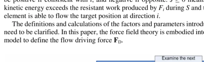
To assess the immunity to noise, a quantitative performance evaluation is also per-formed. The level set method based on regional statistics [6] is chosen for comparison. The test image is generated so that the ground truth segmentation result can be com-pared. The shape of the considered object is designed as a circle with a boundary concavity to increase the detection difficulty. Different levels of Gaussian and Impul-sive noise are added. The mean square error (MSE) is used to measure the performance under noise.

2 1

m a x ( , )

I_D

k D I

k

M S E d I I

=

∑

=

where II and ID are the number of ideal and detected contour points respectively and dk

is the distance between the kth detected contour point and the nearest ideal point. The

quantitative results are shown by figure 4(a) and (b). For both noise, the performance of the water flow model is markedly better than the level set operator especially when the noise contamination is severe (SNR less than 10dB). The performance superiority of the water operator under noisy conditions is further illustrated qualitati- vely by the segmentation results for Gaussian noise (SNR: 13.69) and impulsive noise (SNR: 11.81), see figure 4(c) to (f). This robustness to noise is desirable for many practical applications like medical image segmentation.

(a) (b)

(c) LS (MSE: 0.83) (d) WF (MSE: 0.13) (e) LS (MSE: 1.02) (f) WF (MSE: 0.31)

Fig. 4. Quantitative evaluation and detection examples for level set method (LS) and water flow operator (WF), left for Gaussian noise and right for Impulsive noise

3.2 Natural Images

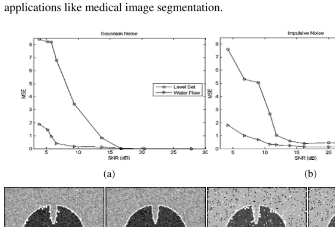
(a) α=0.5, λ=1, k=50

(b) α=0.5, λ=1, k=0

Fig. 5. Water-flow detection results for river delta photo with different parameters: increased λ reduces the significance of image forces, and smaller k makes flow less sensitive to edges, therefore the detail detection level is lower in (b)

Different initializations inside the river were tried and with the same parameters chosen, the results are almost the same, as expected. The operator is insensitive to the source positions. By changing the parameters, however, some alternative results can be achieved. For example, figure 5(b) shows a segmentation of the whole basin of the river. It is analogy to a flood from the river. The water floods the original channels and stops at the relatively high regions. This shows the possibility of achieving different level of detail just by altering some parameters.

(a) (b) (c)

Fig.6. Segmentation results in real medical images: a) brain in a sagittal MR image, b) carotid artery in a MR carotid MRA image and, c) grey/white matter interface in MR brain image slice

tension. The operator can find weak-contrasted boundaries as shown by figure 6(a) where the indistinct interface between the brain and the spine is detected. This is achi- eved by combining a high value of k that gives the operator a high sensitivity to edge response and the region-based forces. The fluidity of water leads to both topological adaptability and geometrical flexibility, and the capillary force assists in detecting narrow tube-like features. Figure 6(b) and (c) illustrate those – the complex structures and irregular branches are segmented successfully.

Retinal vessel segmentation plays a vital role in medical imaging since it is needed in many diagnoses like diabetic retinopathy and hypertension. The irregular and com-plex shape of vessels requires the vessel detector to be free of topology and geometry. Furthermore, digital eye fundus image often have problems like low resolution, bad quality and imaging noise. The water flow model is a natural choice. Figure 7 shows the segmentation results. Multiple initializations/water sources are set inside the vessel

(a) (b)

structures to lighten the problems caused by gaps on the vessels. In figure 7(a), multiple flows of water merged, leading to a single vessel structure. In figure 7(b), some water flows merged and some remained separated. This can be improved by post-processes like gap-linking techniques.

(a)

(b) (c)

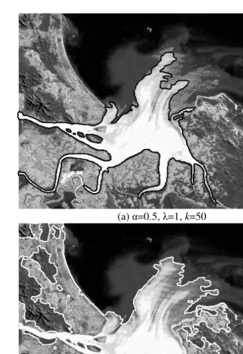
Fig. 8. An example of the MRI volume segmentation by 3-D water flow analogy: a) the water flow model segments the lateral ventricles of brain; b) – c) cross-sections of the results

3.3 Medical Images Volume Segmentation

presents a typical example where the model is applied to a 181×217×181 MR image volume of a human brain. The water source is set inside the lateral ventricles and the parameters are set at k=5, α=0.5, λ=1. The operator detects most parts of the lateral ventricles. Two cross-sections of the fitted model are also shown in figure 8.

4 Conclusions

This paper introduces a new general framework for image segmentation based on a paradigm of water flow. The operator successfully realizes the key attributes of flow process under the structure of force field generation. The resistance given by images is defined by a combination of object boundary and regional information. The problems of boundary concavities and topological changes are settled whist the attractive feature of snakes, the smoothness of the evolving contour, is achieved. Those are approved by the results on synthetic and real images. Good noise immunity is justified both quan-titatively. Besides, the complexity of the algorithm is relatively low. Therefore the method is expected to be of potential use in practical areas like medical imaging and remote sensing where target objects are often complex shapes corrupted by noise. A 3-D version of the operator is also defined and implemented, and is applied to the medical volume segmentation area. The algorithm here uses the simple edge potential forces. In the future we seek to embody more refined edge detectors [15] or new force functionals like GVF [3] into the water flow based framework.

References

[1] Kass, M., Witkin, A., Terzopoulos, D.: Snakes: Active contour models. Int’l. J. of Comp. Vision 1(4), 321–331 (1988)

[2] Cohen, L.D.: On active contour models and balloons, CVGIP. Image Understanding 53(2), 211–218 (1991)

[3] Cohen, L.D., Cohen, I.: Finite element methods for active models and balloons for 2-D and 3-D images. IEEE Trans. PAMI 15, 1131–1147 (1993)

[4] Xu, C., Prince, J.L.: Snakes, shapes, and gradient vector flow. IEEE Trans. Image Proc-essing 7(3), 359–369 (1998)

[5] Figueiredo, M., Leitao, J.: Bayesian estimation of ventricular contours in angiographic images. IEEE Trans. Medical Imaging 11, 416–429 (1992)

[6] Chan, T.F., Vese, L.A.: Active contours without edges. IEEE Trans. Image Processing 10, 266–276 (2001)

[7] McInerney, T., Terzopoulos, D.: T-snakes: topologically adaptive snakes. Medical Image Analysis 4, 73–91 (2000)

[8] Casselles, V., Kimmel, R., Spiro, G.: Geodesic active contours. Int’l Journal of Computer Vision 22(1), 61–79 (1997)

[9] Malladi, R., et al.: Shape modeling with front propagation: A level set approach. IEEE Trans. PAMI 17, 158–174 (1995)

[10] Vincent, L., Soille, P.: Watersheds in digital space: an efficient algorithm based on im-mersion simulations. IEEE Trans. PAMI 13, 583–598 (1991)

[12] Liu, X.U., Nixon, M.S.: Water Flow Based Complex Feature Extraction. In: Blanc-Talon, J., Philips, W., Popescu, D., Scheunders, P. (eds.) ACIVS 2006. LNCS, vol. 4179, pp. 833–845. Springer, Heidelberg (2006)

[13] Liu, X.U., Nixon, M.S.: Water flow based vessel detection in retinal images. In: Proceed-ings of Int’l Conference on Visual Information Engineering, pp. 345–350 (2006)

[14] Hurley, D.J., Nixon, M.S., Carter, J.N.: Force field feature extraction for ear biometrics. Computer Vision and Image Understanding 98, 491–512 (2005)