Symmetry Reduced Model Checking for B

Symmetry Reduced Model Checking for B

Edd Turner

, Michael Leuschel

, Corinna Spermann

, Michael Butler

1

_{School of Electronics and Computer Science}

University of Southampton

SO17 1BJ, UK

{

ent03r,mjb

}

@ecs.soton.ac.uk

2

_{Institut f¨ur Informatik}

Universit¨at D¨usseldorf Universit¨atsstr. 1

D-40225 D¨usseldorf, Germany

{

leuschel,spermann

}

@cs.uni-duesseldorf.de

Abstract

Symmetry reduction is a technique that can help alleviate the problem of state space explosion in model checking. The idea is to verify only a subset of states from each class (or-bit) of symmetric states. This paper presents a framework for symmetry reduced model checking of B machines, which verifies a unique representative from each orbit. Symmetries are induced by the deferred set; a key component of the B language. This contrasts with strategies that require the in-troduction of a special data type into a language, to indicate symmetry. An extended version of the graph isomorphism program, nauty, is used to detect symmetries, and the sym-metry reduction package has been integrated into thePROB model checker. Relevant algorithms are presented, and ex-perimental results illustrate the effectiveness of the method, where exponential speedups are sometimes possible.

1. Introduction

The B-Method [1] is a theory and methodology used for the formal development of computer programs. It includes a concise language based on set theory and predicate logic, called B, and is used by industries in a range of critical do-mains, notably in railway control (e.g., the control system for the automatic, unmanned Paris M´etro Line 14).

Proof activities in B are usually carried out using the in-teractive theorem provers, Atelier-B [25] or the B-toolkit [2]. Model checking is a useful, complementary ap-proach that can perform these tasksautomatically, if bounds are placed on system types; as with the combined B-animation/model checker, PROB [19].

A major challenge facing model checking is the prob-lem of state space explosion. This is where a linear in-crease in the size of a specification leads to an exponential increase in the number of states, which the model checker

must explore. Thus, checking larger specifications becomes intractable. Much research in model checking focuses on methods to combat this problem, including partial order re-duction [12], inre-duction [6] and abstraction [5]. Symmetry reduction is another approach, which exploits symmetries inherent in the system [6] by constraining the search to rep-resentatives of symmetric states; often resulting in signifi-cant savings in memory and time. A successful technique relies on a special data type, called a scalarset, being in-troduced into the language of the model checker, to indi-cate symmetric structures (e.g., the MurϕVerifier [13] and SymmSpin [3]). This requires the user to indicate symme-tries of the model, and is therefore error prone, and compro-mises the automation of model checking.

This paper presents anautomaticmethod for exploiting symmetries caused by a key component of the B language, thedeferred set. The work uses a very different technique to an alternate strategy calledpermutation flooding, which we present in [18]. In the next section, we introduce deferred sets in B, and the notion of symmetry. Section 3 follows with a detailed example that elaborates on the types of sym-metries exploited. The integration of our symmetry reduc-tion into the PROB model checker is given in Secreduc-tion 4. We then describe a two-phase technique that identifies system symmetries, using a graph isomorphism algorithm based on nauty [21]. Finally, we illustrate the effectiveness of the technique by applying it to several typical B models, and we discuss its drawbacks and future improvements.

2. Symmetry and Deferred Sets in B

given below:

SETS

ExitMsg={success,fail}; //an enumerated set Proc//a deferred set

Deferred sets consist of abstract elements. For instance, Procis a set of abstract processors. The only information known about a given element of such a set is theidentityof this deferred set. It follows that the permutation of one ab-stract element for another will have no effect on semantics; no information is gained or lost. Extending this idea, one finds a set containingnelements ofProcto be symmetric to another set containingnelements ofProc. Indeed, the use ofabstractelements in a B specification gives rise to sym-metries in data structures used within the system, which our scheme can exploit. This is similar to the symmetries in-duced by scalarsets [13, 3], which are sets of permutable scalar values. In the next section, we describe a concrete example to elaborate on the types of symmetries that our method can exploit.

3. Motivation

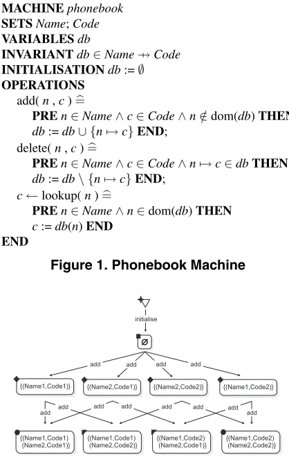
Let us indicate the type of symmetry we want to exploit by considering a simple B model of a phone book, see Fig. 1 below. The model (or machine) has three operations: add, to add entries into the phone book;delete, to remove entries; andlookup, to query a person’s phone number.

The machine has two deferred sets, Name and Code, modelling sets of names and phone numbers respectively. A single variable,db, which is a partial function, stores the contents of the phone book; hence, aNamecan have at most oneCodeassociated with it.

An exhaustive search of the state space of this machine requires bounds to be placed on the types used [19]. If we set the cardinality of the deferred sets to 2, the full state space has 10 distinct states. Fig. 2 shows the state space, where the label of each state is the current value ofdb(e.g.,

{(Name1,Code1)}). For clarity, the parameters of theadd operation are hidden, and thedeleteandlookupoperations are not depicted (this does not affect the set of reachable states).

The use of deferred sets give rise to symmetries among the states. Informally, we define two states as being sym-metric if the machine invariant has the same truth value in both states, and if there is a permutation between the two states that permutes values of deferred sets. We also re-quire this permutation to respect the typing e.g., a Name can only be permuted with another Name. In Fig. 2, the state db = {(Name1,Code1)} is symmetric to db =

{(Name1,Code2)}since both are functions and there is the

MACHINEphonebook

SETSName;Code

VARIABLESdb

INVARIANTdb∈Name →Code

INITIALISATIONdb:=∅

OPERATIONS

add(n,c)=

PREn∈Name∧c∈Code∧n∈/dom(db)THEN

db:=db∪ {n→c}END; delete(n,c)=

PREn∈Name∧c∈Code∧n→c∈dbTHEN

db:=db\ {n→c}END; c←lookup(n)=

PREn∈Name∧n∈dom(db)THEN

c:=db(n)END END

Figure 1. Phonebook Machine

{(Name1,Code1)}

{(Name1,Code1) (Name2,Code1)}

{(Name2,Code1)} {(Name2,Code2)} {(Name1,Code2)}

{(Name1,Code1) (Name2,Code2)}

{(Name1,Code2) (Name2,Code1)}

{(Name1,Code2) (Name2,Code2)} add add add add

add add add add add add add add initialise

Figure 2. State Space of Phonebook

permutation, {(Code1,Code2)} between them. Symmet-ric states in Fig. 2 have been indicated by identical black shapes in their top left hand corner. As can be seen, three other states are symmetric todb={(Name1,Code1)}.

{(Name1,Code1)}

{(Name1,Code1) (Name2,Code1)}

{(Name1,Code1) (Name2,Code2)} initialise

add(Name1,Code1) delete(Name1,Code1)

add(Name2,Code1) add(Name2,Code2)

delete(Name2,Code1) delete(Name2,Code2)

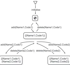
Figure 3. Reduced State Space of Phonebook

Our approach to symmetry reduction checks only one (unique) representative per symmetry class, using an algo-rithm for graph isomorphism that permits the permutations described. For proof of soundness with respect to standard model checking, see [18]. Fig. 3, illustrates the symmetry reduced state space for the phonebook machine. The tech-nique exploits symmetries caused by deferred sets, so it is likely to significantly reduce the time to model check many B specifications, since such sets are commonly used in B. For instance, deferred sets often occur near the top of step-wise refinement chains, in the abstract specifications. In the next section, we present our approach for identifying sym-metries.

4. Symmetry Detection

The task of identifying unique representatives from sets of symmetric states is closely related to the well known problem of solving graph isomorphism [16], which cur-rently has no known polynomial algorithm. However, in practice some extremely efficient algorithms exist for most classes of graphs [15] that may contain several thousands of vertices [11]. The most efficient general purpose graph isomorphism program isnauty[22].

This section outlines our method for computing repre-sentatives of states in B using an extension to the underlying algorithm of nauty. The idea is to compute representatives in two phases, starting by translating a state to a graph, and then applying a graph isomorphism program to find its rep-resentative.

4.1. Symmetry in Model Checking

Let us recall that given a specification of a system, model checking involves the construction of a state transition sys-tem (model), representing the behaviour of the syssys-tem, so

that properties of it can be checked by exhaustive search.

Constructing models inPROB: A specification in B is de-scribed by means of constants and variables, whose evalua-tion determines a state, and a set of operaevalua-tions. To construct the model of a B machine, M, we represent machine con-stants and variables by a vector of variablesV=v₁, . . . ,vn, and we characterise B operations operating on variablesV with inputs x and outputsy by a predicate P(x,V,V,y). Characterising B operations of the form X ← op(Y) as predicates then gives rise to the model: a labelled transition system on states, where statessandsare related by an ope-rationop.a.b, denoteds→M

op.a.b s, whenP(a,s,s,b)holds. A specialrootstate is also added, whereroot→Minitialises de-notes that state ssatisfies the initialisation and properties clause. For further details, see [20]. In PROB, such models are automatically constructed and searched for states that violate properties specified onV (invariant violations), or are deadlocked.

We now formalise our modified model checking algo-rithm, to show how symmetry detection via graph isomor-phism is integrated into the checking; see Algorithm 1. When a new state is encountered it is not explored further if its canonical form has already been explored. On line 4, erroris a function which returns true if the argument is an error state: usually, this means an invariant violation or a deadlock1_{. Also note the use of randomon line 11, and}

α, which is a user defined value. Its effect varies whether model checking progresses using a depth first or breadth first search.

The variableQueue, stores the states with transitions yet to be explored, andV isitedrecords states already reached by checking. SGraphstores the section of the model ex-plored so far. The functionG(line 9) converts a state of a B machine into a labelled, directed graph, and is explained in Section 4.2 below. The functioncanoncomputes a canon-ical form for such a graph. We explain how the function works in Section 4.4. Note that all elements ofQueueand V isitedhave associated hash values. It is therefore usually efficient to decide whethersg∈V isited. We have imple-mented this algorithm within PROB, and we provide empir-ical results later in Section 5.

4.2. The Graph of a B State

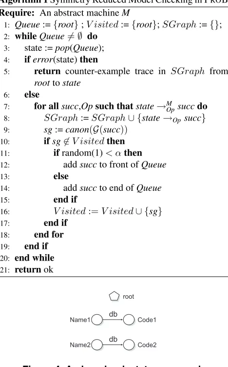
Let us first consider an example of a graph that repre-sents a state, which we will refer to later. Fig. 4 shows the state graph of the state, db = {(Name1,Code1),

(Name2,Code2)}in Fig. 2.

In this graph, the value of the relation,dbis represented by edges that indicate specific ordered pairs, whose edge

1_{We do not deal with liveness properties in this algorithm. In B such}

Algorithm 1Symmetry Reduced Model Checking in PROB

Require: An abstract machineM

1: Queue:={root};V isited:={root};SGraph:={};

2: whileQueue=∅ do

3: state :=pop(Queue); 4: iferror(state)then

5: return counter-example trace in SGraph from

roottostate 6: else

7: for allsucc,Opsuch thatstate→MOpsuccdo

8: _SGraph:=SGraph∪ {state→Opsucc} 9: sg:=canon(G(succ))

10: ifsg∈V isitedthen

11: ifrandom(1)< αthen 12: addsuccto front ofQueue

13: else

14: addsuccto end ofQueue

15: end if

16: _{V isited}:=_{V isited}∪ {sg}

17: end if

18: end for

19: end if

20: end while

21: returnok

Name1

Name2

Code1

Code2 root

db

db

Figure 4. A phonebook state as a graph

labels denote the variable they encode. A special ‘root’ ver-tex is also present (different from the root in Algorithm 1), which is explained later in this section.

Values in B are either elements of sets (including Boolean values and integers), pairs of values, or sets of val-ues. If we first ignore nested values in B, we can use three simple rules to translate a value to its concrete graphical rep-resentation. For an element of a set,v∈S, wherev=s₀, we have the graph in Fig. 5. The graph of a set,v∈P(S), where v = {s₀, . . . ,sn}is shown in Fig. 6. Finally, a re-lation, v ∈ S ↔ T, where v = {(s₀,t₀), . . . ,(sn,tm)} is depicted in Fig. 7. Also, although our graph representation does not distinguish v = {s0} from v = so, the B type system does and we only work with well-typed machines (typing is decidable in B).

We extend this idea for nested data structures, such as sets of sets, through the introduction of a set of special, symmetric vertices X, which contains an element x ∈ X

root

v

s0

Figure 5. Graph for an atom

s0 v

sn

..

v

root

.

Figure 6. Graph for a set

s0 _v t0

root

sn v tm

... ..

. ...

Figure 7. Graph for pairs

for each nested value,V. For nested sets,v={V0, . . . ,Vn}, we createn+ 1 special vertices, and we translate the set

{x₀, . . . ,xn}to a graph, as in Fig. 6. Then, we recurse on each nested valueVi,0≤i≤nand draw the corresponding graph withxias the new ‘root’.

Similarly, for nested relations, v = {(V₀,V₁), . . . ,

(Vn−1,Vn)}, we haven+ 1special vertices, and we trans-late the relation{(x₀,x₁), . . . ,(xn−1,xn)}to a graph, as in Fig. 7. Then, we recurse on each nested valueVi,0≤i≤n and draw the corresponding graph withxias the new ‘root’. By composing the individual graphs that represent each value of a variable in a state, we obtain its state graph. Let G denote the function translating a state to its state graph. As an example, the graphical form of the state,

v1 = {({s0},{s1})}, v2 = {{s2}} is given in Fig. 8. Note that the colours used should be ignored; they will be explained in the next section.

x0 x1

root

s0 s1

v1 v1

v1 x2

s2 v2 v2

Figure 8.G(v₁={({s₀},{s₁})},v₂={{s₂}})

4.3. Relating Graph Isomorphism to

State Equivalence

These algorithms rely on the permutation of graph ver-tices. Let us denote all vertex permutations with the re-lation γ. Now, consider a graph, G with vertices V =

{v₁,v₂, . . . ,vn} and a sequence of vertices v1,v2, . . . ,vn. All n! possible vertex orderings are Γ = {o | o = vγ₁,vγ₂, . . . ,vγn}, each of which corresponds to an adjacency matrix that encodes the graph; thus, Γ is an ordered set. Typically, an implementation of the algorithm will compute a subset ofΓand will choose the least element as the canon-ical label.

The assignment of labels to vertices is one method to en-code extra information in a graph. For example, the vertices of two disjoint sets could be assigned one of two labels. By convention, vertex labels are calledcolours, and a vertex la-belled graph is called acoloured graph. Canonical labels can be computed for coloured graphs by requiring vertex permutations take place over vertices with the same colour.

Definition 4.1 Permutation function canon computes the

canonical label for a coloured graph by permuting vertices with the same colour, such that for two graphsg₁ andg₂, canon(g₁)=canon(g₂)⇔g₁is isomorphic tog₂.

We now describe how coloured graphs relate to state graphs. First, recall that in Section 3 we gave an informal definition of symmetries in B. We say that two states are symmetric if the invariant has the same truth value in both, and there exists a permutation between them over certain elements of deferred sets. In previous work [18], we prove this by defining a permutation function, f over symmetric elements of deferred sets used in a machine.

Definition 4.2LetDSbe the set of disjoint sets in a machine

M. Apermutation f over DSis a bijection from∪S_∈DSSto

∪S_∈DSSsuch that∀S∈DSwe have{f(s)|s∈S}=S.f is a fixpoint for enumerated types, including Boolean values and integers.

We can extend our definition of a state graph (Section 4.2) by colouring vertices. We assign the same colour to any pair of verticesiff f permutes their corresponding state values. For example, the vertex colours used in Fig. 8 would reflect thats₀,s₁∈DS₁ands₂∈DS₂, given thatDS₁,DS₂⊆DS. Also, note the same colour is given to verticesx₀,x₁andx₂, which belong to the set of special, symmetric vertices,X.

By liftingf to machine states we show in [18] that state σ satisfies predicateP (including any invariants), iff f(σ) satisfiesP. The goal now is to show that two states are sym-metriciff canon(G(σ))=canon(G(f(σ))). This is accom-plished sincecanon permutes only vertices with the same colour (Definition 4.1).

State graphs cannot be applied immediately to nauty, which works on undirected, unlabelled and coloured graphs. In the next section we extend this to directed and labelled graphs.

4.4. Computing Canonical Labels for

Unlabelled, Undirected Graphs

The canonicalisation function, canon, has been imple-mented in SICStus Prolog, and integrated into PROB, us-ing a technique called ‘partition refinement’, as used by the efficient graph isomorphism programs of nauty and saucy [8]. For a thorough introduction to partition refinement, see [15, 21]. Our implementation modifies the partition refine-ment step used by nauty. Before explaining our new algo-rithms for computing canonical labels, we first introduce some key concepts, and recall McKay’s algorithm for unla-belled, undirected graphs [21].

A na¨ıve approach to computing canonical labels would maken!analyses for a graph withnvertices (Section 4.3, paragraph 1). Ideally, however, this should be as few as pos-sible. A step towards this goal is to first sort the vertices by degree (the number of adjacent vertices in the graph), and consider only those orderings that preserve the degrees of the vertices. Let us extend this idea with the notion of equi-table partitions; a relatively simple but effective technique that constrains further the number of orderings to consider.

Consider a simple graphGwith the set of verticesV. An ordered partitionπofV is a sequence(V1,V2,· · ·,Vn)of disjoint non-empty subsets ofV, calledcells, whose union is V. A partition is called discrete, if for, 1 ≤ i ≤ n, Vi is trivial(i.e., a singleton set). Let v ∈ V andW ⊆ V, then the number of elements of W, which are adjacent to v inG, is denoted as d(v,W). An ordered partition π is equitableif, for all V₁,V₂ ∈ πandv₁,v₂ ∈ V₁ we have d(v₁,V₂) = d(v₂,V₂). Since discrete partitions contain only trivial cells, we have the property that all discrete par-titions are equitable; however, an equitable partition is not necessarily discrete.

An equitable partition πβ is computed by a procedure

calledrefine, by analysing degrees of vertices in a graph, given some initial ordered partitionπα2. The computation

ensures each cell inπβ is a subset of some cell inπα. πβ

is said to befinerthanπα; denotedπβ ≤πα. Algorithm 2 shows the use ofrefinefor computingcanonical labels.

The functioncompute labelon line 4 is used to encode a graph structure in a non-graphical form. Given a discrete partitionπ, take its adjacency matrix for graphGand define an integern(G)by writing down the entries in the upper-triangle, row by row3_{. Interpreting the result as an n}2

-bit binary string, gives the return value ofcompute label. Furthermore, given a set of discrete partitions, the lexico-graphic order on the corresponding set of binary strings in-duces the presence of a unique, least element, which we take

2_{In the context of partition refinement,refinebares no relation with}

refinement in B.

3_{We only analyse the upper-triangle as undirected graphs have}

Algorithm 2canon(π,G): Computing a canonical label

Require: Unlabelled, undirected graph, G, and ordered

partitionπ

1: πe=refine(π);{refineπto an equitable partition} 2: ifπeis discretethen

3: {compare with smallest label so far} 4: v =compute label(G, πe);

5: ifv≤bestthen

6: best = v;{update label}

7: end if

8: else

9: {_πeis not discrete – attempt to make non-equitable} 10: C= first non-discrete cell inπe;

11: for allu∈Cdo

12: make a copyπuofπein whichCis split intouand C−u

13: canon(πu);

14: end for

15: end if

as the canonical label.

The procedurerefine(line 1) generates for an initial par-tition πα, an equitable partition πβ, such that πβ ≤ πα.

Typically,πβhas significantly more cells thanπα[15], and

consequently,πβhas significantly fewer discrete partitions

(vertex orderings) finer than πα. This premise forms the

basis of Algorithm 2. Starting with an initial partition, cre-ate an equitable, finer partition. If this does not represent a vertex ordering, attempt to make a non-equitable, but finer partition (lines 10-12) and recurse. The overall procedure constructs a search tree, whose leaves are discrete partitions that must be considered when finding the canonical label. The size of the tree is, however, constrained through the use ofrefine, which progressively eliminates a large number of vertex orderings. An in-depth description of this proce-dure, together with algorithmic optimisations, can be found in [21]; for a somewhat gentler introduction, see [23].

In more detail,refine compareseach cell with every other cell inπα. Comparing two cellsV1,V2∈παmeans that for

every elementv∈V₁, we computed(v,V₂). Elements ofV₁ with the same number of edges toV₂form a new cell; thus, V₁is split into several non-empty cells. These cells are or-dered by increasing degree, such that cellVicomes prior to cellVjifdegi≤degj, where∀vi ∈Vi⇒d(vi,V₂) =degi, and∀vj ∈ Vj ⇒ d(vj,V₂) = degj. New partition π_β1 is formed by replacing the cellV1 ∈πα, with the newly cre-ated cells. This process repeats with πβ1 until it remains unchanged or is discrete; the resulting partition,πβis equi-table. For correctness proofs of this procedure, see [21].

New Extended Algorithm: In order to represent the values

of individual variables and constants, as well as to faithfully

represent more complicated B data structures as graphs, we use directed, labelled, coloured (state) graphs. The move to directed graphs is straightforward (mainly consists of using full adjacency matrices in the compute label pro-cedure rather than only triangular ones).Similarly, treating coloured graphs is also not difficult; one simply defines an order on the colours and uses an initial partition where the vertices have already been partitioned according to the var-ious colours (see also [21]). However, the move to graphs with labelled edges is less obvious. Below we describe how we have adapted McKay’s procedure to handle such graphs. The main algorithm for computing the canonical label of a graph with directed and labelled edges is the same except for thecompute labelandrefinesub-procedures.

It should be noted that our implementation ofcanon does notuse several intricate programming optimisations used in nauty (e.g., two variables for all partition nests [21]). Our implementation should be viewed as a proof of concept.

First we describe our change to thecompute label sub-procedure. For labelled edges, an ordering is placed on the set of labelsL(the variable names), so that labelled graphs can be encoded as a single matrix, where each entry is a bi-nary string of size|L|. For directed edges, we ensure com-pute label takes the row-by-row binary string for the full matrix. So for example, in Fig. 8, given a variable order-ingv₁,v₂, the matrix entry at index[x₀,x₁]would be ‘1,0’, since betweenx₀ andx₁ there exists only the single edge labelledv₁.

Algorithm 3 below shows our new refine procedure. Since we work on graphs with directed and labelled edges, we must first adapt the functiond(v,W)and the definition of equitable.

Definition 4.3 Let G be a graph with directed, labelled

edges and set of vertices V, v ∈ V,W ⊆ V and L =

(l₁,· · ·,ll) the labels on the edges. Then din(v,W,l_ν) is the number of elements in W, that have an edge with the labellν ∈Lleading tovanddout(v,W,lν)is the number of elements inW, that have an edge with the labellν coming fromv.

Definition 4.4 Let G be a graph with directed, labelled

edges and set of verticesV andL:= (l₁,· · · ,ll)the labels on the edges. An ordered partitionπof V is calledlabel equitableif, for allV₁,V₂∈π,v₁,v₂∈V₁and labell_ν∈L we have:

din(v1,V2,lν) =din(v2,V2,lν)and dout(v1,V2,lν) =dout(v2,V2,lν).

Example 4.5We shall now integrate the methods described

Algorithm 3refine(π,G): Extended partition refinement

Require: Directed, labelled graphG,π = (V1,· · ·,Vn),

L= (l1,· · · ,ll) 1: ˜π:=π;

2: _α= (V₁,· · · ,Vn);

3: whileπ˜is not discrete andα=∅ do

4: Remove an elementWfromα;

5: for allν ∈1. . .ldo

6: for allk∈1. . .ndo

7: Compute ordered partition (X₁,· · ·,Xs) from Vk, where ∀i,j.1 ≤ i,j ≤ s∧x ∈ Xi∧y ∈ Xj⇒i<j⇔din(x,W,l_ν)<din(y,W,l_ν) 8: ifs>1then

9: update π˜ by replacing the cell Vk with the cellsX1,· · ·,Xs;

10: _α=concatenate(α, (X1,X2,· · ·,Xs));

11: end if

12: end for

13: end for

14: Repeat lines 5 - 13, but use alternate condition dout(x,W,lν)<dout(y,W,lν)on line 7.

15: end while

16: return Label equitable partition,π˜;

x0 x1

root

s0 s1 v1

s2 v2 v2 v1

v2 v2

Order of colours L = (v , )1v2

Figure 9. Example state graph

The example state makes use of two deferred sets,DS₁ and DS₂, and uses two variables, v₁ ∈ P(P(D₁)) and v₂ ∈ P(D₁ ↔ D₂). Let us assume s₀,s₁ ∈ DS₁, s₂ ∈ DS₂, and the variables values v₁ = {{s₀}} and v₂ = {{(s₁,s₂)}}. Note, Fig. 9 also depicts the special verticesx₀,x₁∈Xfor nested values, and the orders of vari-ables and colours. Thus, we start with the initial partition π = ({s₀,s₁},{s₂},{x₀,x₁},{root}), such that vertices in the same cell have the same colour, and the cells are ordered by their colours.

Initially, line 1 of Algorithm 2 requests the partition re-finement of π. We then enter Algorithm 3 with π, and α = ({s0,s1},{s2},{x0,x1},{root}). In the first traver-sal of thewhileloop, W = {s0,s1}. The algorithm con-siders only edges with label v₁ in the first cycle of the outer for-loop. For the first cell of π, V₁ = {s₀,s₁}, no edges labelled v₁ originate fromW and lead to an el-ement of V₁; so din((1),W,a) = din((3),W,a) = 0 and π remains unchanged. The second cell of π, V₂ =

{s2}, is trivial and cannot be split further, so the algo-rithm continues. For the third cell, V3 = {x0,x1}, we have din((x0),W,v1) = 1 > 0 = din((x1),W,v1). So, V₃ is split into two cells, {x₁},{x₀}; which must be or-dered by their values for din. The algorithm updates π andα, whereπ:= ({s₀,s₁},{s₂},{x₁},{x₀},{root})and α:= ({s₂},{x₁,x₀},{root},{x₁},{x₀}). Since the last cell V₄ ={root}is trivial, the algorithm progresses and begins considering edges labelled,v₂(line 5, second iteration).

Splitting next occurs when dout is analysed (execution of line 14), forW = {s₂} and the edge label,v₂. When, V₁ = {s₀,s₁}, we have, dout((s₀),W,v₂) = 0 < 1 = dout((s₁),W,v₂) and so partition π is updated to π :=

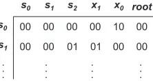
({s₀},{s₁},{s₂}, {x₁},{x₀},{root}), which is now dis-crete. Further splitting is not possible, so Algorithm 3 ter-minates with this discrete, label equitable partition4. With execution returning to line 1 of Algorithm 2, πe is dis-crete and the procedure terminates with the canonical label compute label(Gx, πe). Fig. 10 shows the first two rows of the adjacency matrix ofG, which constitute the twelve most significant bits of the canonical label.

00 00 00 00 00

00 00 00 00

s0 s1 s2 x1 x0 root

s0

s1

. . .

. . .

. . .

. . .

01 01

10

Figure 10. Adjacency matrix corresponding to the canonical label ofGx

5. Empirical Results

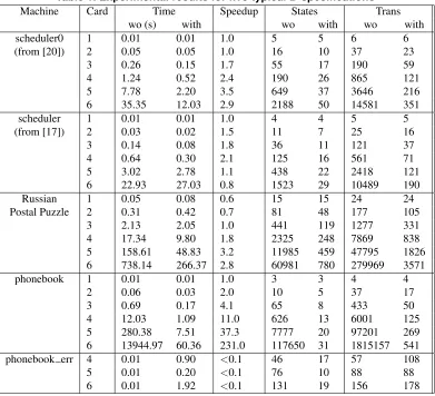
In Table 1 we present the results from applying symme-try reduction in PROB to five typical B specifications. For each specification, we vary the size of deferred sets (Card) and record the time required for model checking to termi-nate. The table also shows the number of states and tran-sitions in the reachable state space, with and without (wo) symmetry reduction. All experiments are performed on a PC with a 2.8GHz Intel Pentium 4 processor, 1Gb of avail-able main memory, running SICStus Prolog 3.12.0 (x86-win32-nt-4) and PROB version 1.2.0. scheduler0 defines a process scheduling specification, and is given in [20]. scheduler is a variation of scheduler0, taken from [17]. The deferred sets in both cases are the process identifiers. Russian Postal Puzzle is a specification of a cryptographic puzzle [10], where the deferred sets are sets of available

4_{Note that a label equitable partition may not be discrete; see}

keys and locks. phonebook is a slightly more elaborate ver-sion of the phonebook defined in Fig. 2, and has 3 variables. phonebook err is the phonebook specification with an error in the precondition of thedeleteoperation, which leads to an invariant violation.

Analysis of the results: Results obtained are

encourag-ing. As can be seen, symmetry reduction reduces verifica-tion time up to some point, in each correct machine. Also, there is a large reduction in the number of states and transi-tions. The most prominent savings are for the phonebook machine, where a linear increase in size of deferred sets leads to a combinatorial saving in time; see the ‘Speedup’ column in Table 1. In the case where deferred sets have a size of 6, reduced checking is 231 times faster than stan-dard checking. The results for the phonebook err machine highlights PROB’s effectiveness at finding counterexam-ples, even without reduction strategies. In fact, symmetry reduced checking requires more time to find the errors (even though fewer states are encountered) due to the overhead of computing representatives. However, the time required was still small (<2s).

Predicting the magnitude of a speedup for some machine is non-trivial since it depends on the behaviour of the ma-chine and the number of elements of deferred sets being used. In all cases, the speedups eventually drop off. The bottlenecks occur when the benefit of performing a con-strained search outweighs the overhead of computing rep-resentatives. Fig. 11 shows how the speedup varies with the size of deferred set, for 3 machines. Data points cor-respond to the cardinality of deferred set used i.e., thenth point on a line shows the speedup when deferred sets con-tainnelement(s). The drop off points illustrated are affected by programming inefficiencies. For instance, the Gauge profiling module in SICStus Prolog shows that more than 70% of computation time is spent accessing Prolog terms that model arrays; this figure would besignificantlyreduced if C-language arrays were used, which have constant-time access. Additionally, several major optimisations used in nauty are not used by our algorithm. The result of any al-gorithmic optimisation would be to increase the speedups achieved (i.e., increase the gradient of lines in Fig. 11) and delay the speedup drop off points.

6. Related Work

Symmetry reduction in model checking dates back to [4, 3], and more recently [9]. A key difference with these works is that ours does not consider temporal logic formu-las, but B’s criteria of invariant violations, deadlocks and refinement. Despite this, the fundamental problem of ef-ficiently computing representatives, namely the orbit prob-lem, is common to all approaches.

The line of research that has developed symmetry

reduc-10-1 100 101 102 103

100 101 102 103 104 105 106

Speedup (log)

Reachable States (log)

scheduler0 Russian Post Puzzle phonebook

Figure 11. Variation of speedups with cardi-nality of deferred sets

tion techniques based onscalarsets[13] is the inspiration for the present article. The SymmSpin package [3] uses scalarsets to integrate symmetry reduction into the SPIN model checker. These special types contain only symmetric data values and are thus similar to deferred sets in B. How-ever, the scalarsets approach is not automatic; it requires the user to identify and assert the presence of symmetries. Our approach is fully automatic since the deferred set is a key component of the B language. Furthermore, our reduc-tion strategy will always apply to a large proporreduc-tion of B machines since deferred sets are frequently used.

In Section 4.2, we show how to encode a B state as a graph. Various other research also addresses this general problem, such as [24], which describes an approach for states of Java programs. For each Java object one encodes its associated type (or program counter, if it is a thread), and a finite set of values. The state graph, orshape graph, is then a directed, labelled graph, which intuitively repre-sents the state’s contents, and which also makes use of a root node. This differs from B state graphs as shape graphs are entirely deterministic, except for the use of special transitions (i.e., indistinguishable labels that can indicate nodes corresponding to active threads) – both features are not present in B state graphs. In addition, B state graphs encode non-comparable abstract elements of deferred sets, for which there is no equivalent notion in Java. However, it remains that both methods share the use of state/shape graphs to achieve the goal of exploiting symmetries in their respective systems.

sym-Table 1. Experimental results for five typical B-specifications

Machine Card Time Speedup States Trans

wo (s) with wo with wo with

scheduler0 1 0.01 0.01 1.0 5 5 6 6

(from [20]) 2 0.05 0.05 1.0 16 10 37 23

3 0.26 0.15 1.7 55 17 190 59

4 1.24 0.52 2.4 190 26 865 121

5 7.78 2.20 3.5 649 37 3646 216

6 35.35 12.03 2.9 2188 50 14581 351

scheduler 1 0.01 0.01 1.0 4 4 5 5

(from [17]) 2 0.03 0.02 1.5 11 7 25 16

3 0.14 0.08 1.8 36 11 121 37

4 0.64 0.30 2.1 125 16 561 71

5 3.02 2.78 1.1 438 22 2418 121

6 22.93 27.03 0.8 1523 29 10489 190

Russian 1 0.05 0.08 0.6 15 15 24 24

Postal Puzzle 2 0.31 0.42 0.7 81 48 177 105

3 2.13 2.05 1.0 441 119 1277 331

4 17.34 9.80 1.8 2325 248 7869 838

5 158.61 48.83 3.2 11985 459 47795 1826

6 738.14 266.37 2.8 60981 780 279969 3571

phonebook 1 0.01 0.01 1.0 3 3 4 4

2 0.06 0.03 2.0 10 5 37 17

3 0.69 0.17 4.1 65 8 433 50

4 12.03 1.09 11.0 626 13 6001 125

5 280.38 7.51 37.3 7777 20 97201 269

6 13944.97 60.36 231.0 117650 31 1815157 541

phonebook err 4 0.01 0.90 <0.1 46 17 57 108

5 0.01 0.20 <0.1 76 10 88 88

6 0.01 1.92 <0.1 131 19 156 178

metries being computed through the addition of predicates that constrain the search. Although originally aimed at SAT based search methods, the key ideas appear applicable to a constraint logic programming environment such as SICStus Prolog, as used by PROB.

7. Conclusions and Future Work

In this paper, we have presented the first technique to achieve classical symmetry reduction for model checkers of B specifications. The algorithm computes representatives in two phases. First we compute the state graph of states, and then we compute its canonical label, corresponding to the unique representative ofs. We have described the relation of symmetries in B to canonical labelling algorithms, and have presented a translation of B states to graphs. We have also presented our extension to McKay’s algorithm to find canonical labels. We have implemented the algorithm in-side the PROB toolset and have evaluated the approach on a

search spacebeforesymmetric states are encountered.

References

[1] J. R. Abrial.The B Book: Assigning programs to meanings. Cambridge University Press, New York, NY, USA, 1996. [2] B-Core (UK) Limited, Oxon, UK. B-Toolkit, On-line

man-ual, 1999.

[3] D. Bosnacki, D. Dams, and L. Holenderski. Symmetric SPIN. STTT International Journal on Software Tools for Technology Transfer, 4(1):92–106, 2002.

[4] E. M. Clarke, T. Filkorn, and S. Jha. Exploiting symmetry in temporal logic model checking. In C. Courcoubetis, edi-tor,CAV, volume 697 ofLecture Notes in Computer Science, pages 450–462, London, UK, 1993. Springer-Verlag. [5] E. M. Clarke, O. Grumberg, and D. E. Long. Model

check-ing and abstraction. ACM Trans. Program. Lang. Syst., 16(5):1512–1542, 1994.

[6] E. M. Clarke, O. Grumberg, and D. Peled. Model checking. The MIT Press, 1999.

[7] J. M. Crawford, M. L. Ginsberg, E. M. Luks, and A. Roy. Symmetry-breaking predicates for search problems. InKR, pages 148–159, 1996.

[8] P. T. Darga, M. H. Liffiton, K. A. Sakallah, and I. L. Markov. Exploiting structure in symmetry detection for CNF. In S. Malik, L. Fix, and A. B. Kahng, editors,DAC, pages 530– 534. ACM, 2004.

[9] A. F. Donaldson and A. Miller. Exact and approximate strategies for symmetry reduction in model checking. In J. Misra, T. Nipkow, and E. Sekerinski, editors,FM, volume 4085 ofLecture Notes in Computer Science, pages 541–556. Springer, 2006.

[10] S. Flannery and D. Flannery. In Code: A Mathematical Journey. Algonquin Books of Chapel Hill, Chapel Hill, NC, USA, 2001.

[11] P. Foggia, C. Sansone, and M. Vento. A performance com-parison of five algorithms for graph isomorphism. In3rd IAPR TC-15 Workshop on Graph-based Representations in Pattern Recognition, 2001.

[12] G. J. Holzmann and D. Peled. An improvement in formal verification. In D. Hogrefe and S. Leue, editors,FORTE, volume 6 ofIFIP Conference Proceedings, pages 197–211. Chapman & Hall, 1994.

[13] C.-W. N. Ip and D. L. Dill. Better verification through sym-metry. In D. Agnew, L. J. M. Claesen, and R. Camposano, editors,CHDL, volume A-32 ofIFIP Transactions, pages 97–111. North-Holland, 1993.

[14] D. Jackson. Software Abstractions: Logic, Language, and Analysis. MIT Press, 2006.

[15] W. Kocay. On Writing Isomorphism Programs, chapter Chapter 6, pages 135–175. Computational and Constructive Design Theory. Kluwer, 1996.

[16] D. L. Kreher.Combinatorial Algorithms: Generation, Enu-meration and Search. Discrete Mathematics and its Appli-cations. CRC Press, 1998.

[17] B. Legeard, F. Peureux, and M. Utting. Automated boundary testing from Z and B. In L.-H. Eriksson and P. A. Lindsay, editors,FME, volume 2391 ofLecture Notes in Computer Science, pages 21–40. Springer, 2002.

[18] M. Leuschel, M. Butler, C. Spermann, and E. Turner. Sym-metry reduction for B by permutation flooding. In J. Julliand and O. Kouchnarenko, editors,B, volume 4355 ofLecture Notes in Computer Science, pages 79–93. Springer-Verlag, 2007.

[19] M. Leuschel and M. J. Butler. ProB: A model checker for B. In K. Araki, S. Gnesi, and D. Mandrioli, editors,FME, volume 2805 ofLecture Notes in Computer Science, pages 855–874. Springer, 2003.

[20] M. Leuschel and M. J. Butler. Automatic refinement check-ing for B. In K.-K. Lau and R. Banach, editors,ICFEM, volume 3785 ofLecture Notes in Computer Science, pages 345–359. Springer, 2005.

[21] B. D. McKay. Practical graph isomorphism. In Numeri-cal mathematics and computing, Proc. 10th Manitoba Conf., Congr. Numerantium 30, pages 45–87, 1981.

[22] B. D. McKay. NAUTY user’s guide (version 1.5), Technical report TR-CS-90-02. Australian National University, Com-puter Science Department, ANU, 1990.

[23] T. Miyazaki. The complexity of Mckay’s canonical label-ing algorithm. In L. Finkelstein and W. M. Kantor, edi-tors,Groups and Computation II, volume 28 ofDIMACS Series on Discrete Mathematics and Theoretical Computer Science, pages 239–256. American Mathematical Society, Providence, Rhode Island 02940, USA, 1997.

[24] Robby, M. B. Dwyer, J. Hatcliff, and R. Iosif. Space-reduction strategies for model checking dynamic software. Electr. Notes Theor. Comput. Sci., 89(3), 2003.