Design optimisation of electromagnetic devices using continuum design sensitivity analysis combined with commercial EM software

Design optimisation of electromagnetic devices using

continuum design sensitivity analysis combined with

commercial EM software

D.-H. Kim, J.K. Sykulski and D.A. Lowther

Abstract:The paper deals with two types of optimisation problem: optimised source distribution and the shape optimum design, using continuum design sensitivity analysis (CDSA) in combination with standard electromagnetic (EM) software. Fast convergence and compatibility with existing EM software are the distinctive features of the proposed implementation. To verify the advantages and also to facilitate understanding of the method itself, two design optimisation problems have been tested using both 2D and 3D models: the first is an MRI design problem related to finding an optimum permanent magnet distribution, and the second is a pole shape design problem to reduce the cogging torque in a BLDC.

1 Introduction

The concept of continuum design sensitivity analysis (CDSA) was introduced in the late 1980s and successfully applied to the design of electromagnetic (EM) devices. However, CDSA provides a methodology in which the elec-tromagnetic analysis can be considered to be a ‘black box’, i.e. the internals of the EM analysis system are irrelevant, and the CDSA method only requires the inputs and outputs of the system. This feature of CDSA makes it, potentially, extremely powerful and creates a simple inter-face with existing analysis packages [1, 2]. Recently, the physical meaning of pseudosources of an adjoint system in CDSA when applied to shape optimisation was explored

[3], and the approach was reported to avoid the need for access to source code of commercial programs. Moreover, the computing times required to find an optimum solution were found not to be affected by the number of design vari-ables. The initial, very encouraging, results have prompted researchers to pursue this technique further as it appears to be competitive compared, for example, with stochastic methods[4].

In this paper, the CDSA method originally introduced in our previous paper [3] is extended to cover two types of optimisation problem; moreover, a unified program archi-tecture in combination with commercial electromagnetic software (on this occasion two programs called OPERA and MagNet, respectively, were used) is presented, to aid the design optimisation of electromagnetic devices. The two problems can be categorised as topology optimisation (TO) and shape optimum design (SOD) and generally

they are considered to be different from each other. However, from the viewpoint of the derivation and implementation of a design sensitivity formula, it is noticed that they follow a very similar procedure [3, 5]. Thus, after minor modifications to a part of the optimisation module of TO, the same program architecture can be applied to SOD problems.

Finally, so that we can verify the advantages of CDSA, the problems are tested by the use of CDSA in conjunction with different EM software. In addition, with the view of facilitation of an understanding of the method itself, a more general and very common program architecture con-sisting of MS Excel spreadsheets and the Visual Basic (VB) editor is attempted.

2 Affinities of two optimisation problems

As stated above, in this paper, the optimisation problems related to TO and SOD are compared with each other in terms of both the derivation and implementation of the two design sensitivity formulae based on the concept of CDSA. It will be shown that the two problems can be dealt with using the same program architecture, with only minor modifications to the optimisation code.

2.1 Procedure of deriving two design sensitivity formulae

In CDSA, the derivation of the sensitivity formula always starts from the variational form of Maxwell’s equations, referred to as the primary system. This fact can easily be overlooked but it does give CDSA a distinctive feature of being adaptable to various analysis tools, such as the finite-element method (FEM), boundary-element method (BEM), finite difference method (FDM) and so on.

Somewhat complicated mathematical expansions are needed to produce the analytical sensitivity formula, but they follow a fairly routine procedure, illustrated in

Fig. 1, where the augmented Lagrangian method (ALM), the material derivative concept and the adjoint variable method (AVM) are exploited. It is well known that the analytical formula facilitates calculation of the first-order

#The Institution of Engineering and Technology 2007 doi:10.1049/iet-smt:20060024

Paper first received 6th March and in revised form 28th June 2006

D.H. Kim is with the School of Electrical Engineering & Computer Science, Kyungpook National University, Daegu 702-701, Korea

J.K. Sykulski is with the School of Electronics & Computer Science, University of Southampton, Southampton SO17 1BJ, UK

D.A. Lowther is with the Department of Electrical & Computer Engineering, McGill University, Montreal, Quebec, Canada, H3A 2A7

gradient information of an objective function with respect to shape design variables and can also save a lot of computing time in the search for an optimum solution, especially as the number of design variables increases. So that the advan-tages of CDSA could be utilised, the generalised analytical sensitivity formulae for the SOD of magnetostatic and elec-trostatic problems were developed, and the effectiveness was verified for a range of design problems[6, 7].

The main approach to the development of an analytical sensitivity formula for TO has been the use of the Tellegen theorem, or the ‘mutual energy’ concept, in con-junction with AVM [8, 9]. However, it is recognised that the meaning and physical interpretation of the adjoint system in such formulations are often obscure and thus dif-ficult to understand. To overcome the drawbacks, the same procedure as presented inFig. 1was successfully applied to TO for the derivation of a unified design sensitivity formula with respect to the system parameters of magnetic materials and sources [5]. The main difference in the derivation process in TO is that the material derivative in SOD is replaced with the first variation of an objective function. As a result, it is revealed that there exists a distinction between the optimised material distribution (OMD) and the optimised source distribution (OSD) forms of TO.

2.2 Mathematical expressions for the two design sensitivity formulae

For the similarity between TO and SOD to be examined explicitly, it is necessary to compare the mathematical expressions of the two sensitivity formulae derived for mag-netostatic design problems. To facilitate understanding, a brief review of the sensitivity formulae derivation from the point of view of CDSA will first be given.

When we are dealing with the variation of an objective function, in response to changes in the shape and material properties, it is convenient to think of the analysis domain as a continuous medium and utilise the material derivative idea of continuum mechanics [5, 6]. Thus the material derivative concept with ALM and AVM is used as a common vehicle to develop both the sensitivity formulae.

For the derivation of the sensitivity formula, an objective functionFis mathematically expressed as

F ¼

ð

V

gðAðpÞ;curlAðpÞÞdV ð1Þ

wheregmeans a scalar function differentiable with respect to the magnetic vector potential, A and curlA, which are themselves implicit functions of the design variable vector

p. So that the sensitivity formula and the adjoint system equation can be deduced systematically, the variational form of the Maxwell’s equation of the primary system is

added to (1) based on ALM. Thus

F¼

ð

V

gðA;curlAÞdV

þ

ð

V

l½curlðncurlAMÞ þJdV ð2Þ

wherenis the reluctivity, andlmeans the Lagrange multi-plier vector interpreted as the adjoint variable.

The mathematical process described above is applied to the derivation of the sensitivity formulae for both SOD and TO, but, depending on which kind of design variable is selected, their final sensitivity expressions have slightly different forms to each other.

In the case of SOD, for an explicit sensitivity expression to be obtained for the deformation of the interface boundary between different materials, the material derivative is taken on both sides of (2) with respect to the shape changes. After exploitation of some mathematical manipulations, as detailed in [3, 6], the final design sensitivity formula (3) for SOD is obtained in the form of surface integration along the moveable boundary g between two different materials, denoted by subscripts 1 and 2, respectively. In (3), pis a design variable vector relevant to the geometry of the design model, and Vn is a design velocity vector normal to g. To simplify the comparison, the additional terms of the generalised expression given in[6]are omitted. On the other hand, a unified sensitivity formula (4) appli-cable to TO is obtained by the taking of the first variation of

Fig. 1 Procedure for deriving sensitivity formulae for SOD

and TO

Fig. 2 Flowchart of SOD and TO using CDSA

both sides of (2) with respect to small changes dpof the system parameters of magnetic materials and sources [5]. As a result, p in (4) is composed of permeability m, current densityJand permanent magnetisationMassigned to design regions of interest.

dF dp¼

ð

g

½ðn₁n₂ÞcurlA₁curll₂

þ ðJ₂J₁Þ l₂þ ðM₂M₁Þ curll₂V_ndG ð3Þ

dF dp¼

ð

V @v

@p

curlAcurllþ@J @pl

þ@M @p curll

dV ð4Þ

If we compare (3) and (4), it can be seen that the three integrands consisting of the sensitivity coefficients with respect to shape or material design variables have very similar forms in their corresponding terms. The only differ-ences are that the surface integral is needed for the SOD form, and the volume integral is needed for TO, and, additionally, the partial derivatives of the system par-ametersm,J, andMare required in the case of TO.

2.3 Numerical implementation

Using the analytical formulae (3) and (4), the first-order gra-dient information of an objective function with respect to the design variables for SOD and TO can be easily calcu-lated from the field and potential values obtained in the dual solution system consisting of the primary and adjoint systems, that is from the results of the analyses. Therefore the solution of the adjoint system, the counterpart of the primary system, is the core of the implementation of an optimisation technique based on CDSA. For this reason, in a previous paper[3], the physical meaning of the pseudo-sources and a direct method of constructing the adjoint system were thoroughly investigated and successfully incorporated into the FE model without any amendments to the software source code.

As part of our continuing work on CDSA, a unified program architecture applicable to both TO and SOD is pre-sented in this paper. According to the similarities between the two optimisation problems discussed so far, the program consists of two independent modules that are dis-tinguished by the dotted box shown in Fig. 2. The

optimisation module outside the box controls the overall design procedure and evaluates crucial quantities such as the objective functions, adjoint source terms and design sen-sitivity. On the other hand, the analysis module inside the box estimates the performance of the dual system whenever the design variables change. It should be noted that the two modules are constantly communicating with each other and exchanging information about design variables, regions of interest and state variables through the API and the command language supported by EM software packages.

Under the proposed program architecture, the iterative design process for TO and SOD involves the following steps.

Step 1: Define an objective function and design variables (TO: topological data, SOD: geometric data).

Step 2: Build an FE model of the primary system so that changes in design variables can be reflected in each design process.

Step 3:Solve the primary system.

Step 4: Store post-processing data (FE results) of the primary system.

Step 5:Calculate the objective function and adjoint forcing terms based on the FE results of the primary system. Step 6:Build an FE model of the adjoint system where most of the model data are inherited from those of the primary system.

Step 7:Solve the adjoint system.

Step 8:Store the post-processing data of the adjoint system. Step 9:Compute design sensitivities and the objective func-tion from FE results of the dual system.

Step 10:Repeat the above procedure from steps 2 to 9 until the objective function converges.

It is worth emphasising again that the main advantage of our proposed approach is the ease of implementation, especially in combination with commercial finite element software. The actual performance of the CDSA-based optimisation will be comparable with other deterministic methods in terms of computing times and accuracy, but with the

Fig. 4 Convergence of objective function against iterations

a

b

c

d

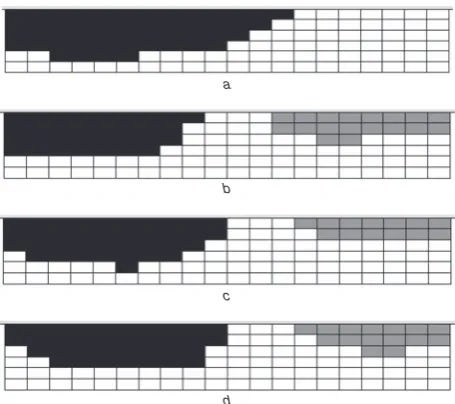
Fig. 5 Changes is shimming magnet distribution during

optimisation

BþMs B2Ms

a 1 iteration

b 3 iterations

c 7 iterations

significant advantage of not requiring a direct derivative of the FE system matrix, which is the essence of other methods based on discrete formulation. The application of stochastic optimisers, on the other hand, would increase computing times dramatically.

3 Case studies

The proposed program architecture was successfully applied to TO and SOD problems in conjunction with two different commercial EM software packages, i.e. OPERA

[10] and MagNet [11], without the need for the source code to be modified. So that we could verify the advantages and also to facilitate an understanding of the method itself, two design optimisation problems were tested: one is an MRI design problem related to the search for an optimum permanent magnet distribution to produce a particular field uniformity, and the other is a pole shape design problem for a BLDC motor intended to reduce the cogging torque, based on both 2D and 3D models.

3.1 Topology optimisation of an MRI

At the stage of definition of an FE design model for TO in

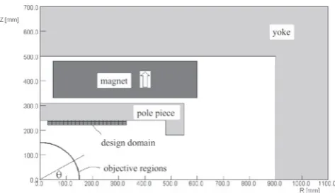
Fig. 2, the design domain to be occupied by materials should be subdivided into multiple individual regions, so that material properties can be imposed in each region defined prior to FE mesh generation. The individual regions correspond to design cells, and a linear static OPERA-2D solver was used for analysis. In the case of OPERA, the command files and input/output data files containing design information and FE results play an important role in the interface between the optimisation module and the analysis module. Fig. 3 shows a quarter of a model of a permanent magnet assembly for an MRI device where the residual flux density of the magnet is 1.21 T [5]. Although the actual assembly is three-dimensional, as it has two columns, here it has been sim-plified to an axisymmetric problem. The design goal is to find an optimised distribution of shimming magnets over the pole piece surface to produce homogenous field distri-bution in a 30 cm diameter spherical volume (DSV). The shimming magnet has a residual flux density of 0.22 T and thickness of 3 mm, and the domain is subdivided into 120 separate regions.

If the TO algorithm is used especially for optimising the source distribution presented in[5], the objective function and design variable are defined as

F¼X

45

i¼1

ðH_ziH_zoÞ2 Mðx;yÞ ¼M_sðPÞ ð5Þ

whereHziis thez-component of the magnetic field intensity computed over the objective regions (consisting of 45 indi-vidual quadrilateral regions along a 908 arc at a 300 mm radius), andHzois the desired value. In (3),Ms(P) in each cell is set to have a value of +Ms, according to the sign of the accumulated design sensitivityPduring optimisation, to take into account the direction ofMs. The algorithm was executed under initial conditions of the desired volume Vo¼42% of all design cells, and the mutation factor

gmax¼20%. The factorgis used in the material updating

Fig. 6 Comparison of field distributions before and after

optimisation

process to avoid oscillations in convergence that can occur if too many cells are changed on each iteration. The mutation factor is gradually reduced from the maximum value to zero during the optimisation process. The sensi-tivity coefficients are evaluated from the analytical formula (4) using the two results from the dual systems in the iterative design process.

The convergence of the objective function and the shim-ming magnet distribution during the optimisation are shown inFigs. 4and5, respectively. Note that convergence actu-ally occurs at iteration 10, and the system oscillates after this point by continually switching the values of a few cells. Fig. 6compares thez-component of magnetic fields over the surface of the DSV before and after optimisation, where the uniformity of the fields is improved four-fold compared with the initial design.

3.2 Shape optimisation of a motor

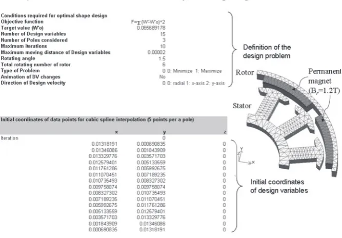
As shown in Fig. 7, a BLDC motor with eight permanent magnets and 12 salient stator poles was considered, and optimisation was carried out to minimise the cogging torque, the magnitude of which reaches nearly 15% of the rated torque. The outer radii of the stator teeth, magnet and rotor yoke are 13.8 mm, 15.3 mm and 16 mm, respect-ively. The depth of the teeth is 2.5 mm, whereas that of the magnet and the yoke is 3.8 mm. Only one-eighth of the problem needed to be modelled owing to symmetry.

In this problem, the fringing effect of the magnetic field can have a large impact on the cogging torque and, because of the geometry of the motor, the three-dimensional fringing is likely to be extremely important. Thus it is necessary to look at both 2D and 3D solutions to the problem. Fig. 8 Design variables in 2D and 3D optimisation

a 33 vertices in 2D

b165 vertices in 3D

The optimisation of the pole face shape was performed using the program architecture of Fig. 2 in conjunction with commercial software (MagNet 6). Each pole face in the 2D shape optimisation is described by 11 finite element vertices forming the outline of the stator pole, as in

Fig. 8a. To prevent a saw-toothed pole face shape, a cubic spline interpolation curve was introduced [12]. Thus the movement of the five control points marked with dotted circles on the pole face in Fig. 8a constrains their corre-sponding 11 vertices to be positioned on a smooth curve.

So that manufacturing limitations can be taken into account, a geometrical constraint that all the pole face shapes should be identical and each should be symmetric is imposed on the design variables when points are moved in the radial direction. For a 3D shape optimisation with a spline parameterisation to be achieved, the stator was decomposed into four independent layers with a thickness of 0.3125 mm (Fig. 8b) and the common surface of adjacent layers was allowed to be deformable to facilitate the confor-mity of the FE mesh with the continuing shape changes. The reduction of the cogging torque was accomplished by (6) expressing the variation of the co-energy stored in a mag-netic system against the rotor positions.

F¼X

nr

i¼1

ðW_iW_oÞ2 ð6Þ

wherenris the number of rotor positions considered,Withe stored co-energy computed at the ith position, and Wo is the constant target value. Owing to the 158periodicity of the cogging torque, the objective function is calculated every 1.58, from 08, to 158, in both 2D and 3D non-linear FE analyses. It should be noted that, in the case of the objective function (6) expressed in terms of system energy, the adjoint system is identical to the primary system, and thus there is no need to solve a second problem to implement the CDSA approach

[3, 6]. In other words, the sensitivity coefficients are evaluated from the analytical formula (3) using the FE results of only the primary system in the iterative design process. However, the purpose of this example is to provide a more general frame-work for design optimisation, using CDSA with the level of flexibility required to tackle other design problems.

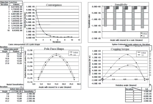
The design details necessary for pole shape optimisation are contained in the MS Excel spreadsheets, as shown inFig. 7, and the VB script file, containing an optimisation algorithm and command language used in the FE software, controls the overall design procedure. At each stage of the iterative design process, information about changes to geometric

parameters and performance data are stored and visualised graphically on the Excel spreadsheets, as shown inFig. 9.

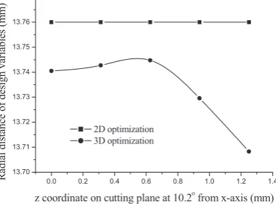
After ten iterations in 2D and 11 in 3D, the optimum pole face shapes were achieved. Fig. 10 shows the difference between the pole face shapes optimised using 2D and 3D analyses on a cutting plane parallel to the z-axis and located at 10.28from thex-axis. A 3D model was created by an extrusion technique from the 2D optimised pole shape, and a comparison of the cogging torque waveforms obtained from the 2D and 3D optimised pole shapes is shown in Fig. 11. It is clear that the 3D optimised pole reduces the cogging torque by 30% of the initial value, whereas the 2D analysis suggests only a 16% reduction. This difference is due to the significance of the fringing effect in the 3D model.

4 Conclusions

A flexible program architecture combining standard FE software packages with command language, MS Excel spreadsheets or Visual Basic script is proposed, with the aim of aiding the efficient solution of design optimisation problems for both TO and SOD. Examples related to determination of the optimum permanent magnet distribution in an MRI system and minimisation of the cogging torque of a BLDC motor have been given. The results show that CDSA is a very efficient optimisation technique offering much reduced computational effort, owing to the fact that computing times do not depend on the number of design variables.

5 Acknowledgments

This work has been supported by KESRI (R-2005-7-041), which is funded by the Ministry of Commerce, Industry & Energy (MOCIE).

6 References

1 Park, I., Coulomb, J.L., and Hahn, S.: ‘Implementation of continuum sensitivity analysis with existing finite element code’,IEEE Trans. Magn., 1993,29, pp. 1787 – 1790

2 Park, I., Lee, H., Kwak, I., and Hahn, S.: ‘Design sensitivity analysis for steady state eddy current problems by continuum approach’,IEEE Trans. Magn., 1994,30, pp. 3411 – 3414

3 Kim, D., Ship, K., and Sykulski, J.K.: ‘Applying continuum design sensitivity analysis combined with standard EM software to shape optimisation in magnetostatic problems’,IEEE Trans. Magn., 2004, 40, pp. 1156 – 1159

4 Farina, M., and Sykulski, J.K.: ‘Comparative study of evolution strategies combined with approximation techniques for practical electromagnetic problems’, IEEE Trans. Magn., 2001, 37, pp. 3216 – 3220

0.0 0.2 0.4 0.6 0.8 1.0 1.2 1.4 13.70 13.71 13.72 13.73 13.74 13.75 13.76 13.77 R

adial distance of

design variables (m

m

)

z coordinate on cutting plane at 10.2o from x-axis (mm)

2D optimization 3D optimization

Fig. 10 Comparison of optimised shapes from 2D and 3D

analyses

0.0 1.5 3.0 4.5 6.0 7.5

-1 0 1 2 3 4 5 6 7 C ogg ing tor que ( g -c m )

Rotating angle (degree)

Initial

3D model based on 2D optimization 3D optimization

Fig. 11 Cogging torque waveforms for initial, 2D and 3D

5 Kim, D., Sykulski, J.K., and Lowther, D.A.: ‘A novel scheme for material updating in source distribution optimisation of magnetic devices using sensitivity analysis’, IEEE Trans. Magn., 2005, 41, pp. 1752 – 1755

6 Kim, D., Lee, S., Park, I., and Lee, J.: ‘Derivation of a general sensitivity formula for shape optimisation of 2-D magnetostatic systems by continuum approach’, IEEE Trans. Magn., 2002, 38, pp. 1125 – 1128

7 Kim, D., Park, I., Shin, M., and Sykulski, J.K.: ‘Generalized continuum sensitivity formula for optimum design of electrode and dielectric contours’,IEEE Trans. Magn., 2003,39, pp. 1281 –1284

8 Dyck, D.N., Lowther, D.A., and Freeman, E.M.: ‘A method of computing the sensitivity of electromagnetic quantities to changes in material and sources’,IEEE Trans. Magn., 1994,30, pp. 3415 – 3418 9 Byun, J., Hahn, S., and Park, I.: ‘Topology optimization of electrical devices using mutual energy and sensitivity’,IEEE Trans. Magn., 1999,35, pp. 3718 – 3720

10 Vector Fields Limited: ‘OPERA User’Guide’, 2005 11 Infolytica Corporation: ‘MagNet 6 User’s Guide’, 2005

12 Kim, C., Lee, H., and Park, I.: ‘B-spline parameterization of finite element models for optimal design of electromagnetic devices’,