Concurrent Q Learning for Autonomous Mapping and Navigation

Concurrent Q-Learning for Autonomous Mapping and Navigation

R.B. Ollington and P. W. Vamplew

School of Computing, University of Tasmania, Tasmania, Australia {Robert.Ollington, Peter.Vamplew}@utas.edu.au

Abstract

This paper presents a new algorithm for goal-independent Q-learning. The model was tested on a simulation of the Morris watermaze task. The new model learns faster than conventional Q-learning and experiences no interference when the goal location is moved. Once the new location is discovered the system is able to navigate directly to the platform on subsequent trials. The model was also tested on watermaze tasks involving barriers. The presence of barriers did not affect the acquisition of “one-trial” learning. While presented as a navigational and mapping technique, the model could be applied to any reinforcement learning task with a variable reward structure.

1.

Introduction

Reinforcement learning (RL) techniques such as Temporal Difference learning (TD)[1] have been shown to display good performance in tasks involving navigation to a fixed goal[2, 3]. If the goal location is moved, however, the previously learnt information interferes with the task of finding the new goal location and performance suffers accordingly[3].

Rats do not exhibit this limitation and have been shown to achieve “one-trial” learning in tasks where the goal location is moved after learning to navigate to a previous location. In the reference memory watermaze task (RMW)[3-5] rats are trained to find the location of a hidden platform in a circular pool over a period of several days, undergoing four trials per day. After this initial training period the platform is moved to a new location. Once the new platform location is discovered the rats are able to navigate directly to the new location on subsequent trials.

In the delayed matching-to-place task (DMP)[3, 4] the platform is moved at the end of every day and even in this more complex task the rats are able to achieve “one-trial” learning after very few days. Typical results for the RMW and DMP tasks are shown in Figure 1.

A crucial component of the rat’s spatial ability is the hippocampus and in particular the place cells[6, 7] found predominantly in areas CA1 and CA3. These cells fire whenever the rat is located at or near a particular location within its environment, or more accurately, they predict the future location of the rat on a short time scale

(~100ms)[8]. The region where the activity of a place cell is high is called the cell’s place field.

a)

[image:1.612.325.554.182.520.2]

b)

Figure 1. Performance of rats on: a) the RMW watermaze task where the platform is moved on day eight; and b) the DMP watermaze task where the platform is moved at the beginning of each day[3, 4].

Recently, neurons have been found in the basal ganglia whose firing patterns show a striking similarity to the TD error term[9-11]. Moreover, it is known that there is considerable connectivity between the hippocampus and the basal ganglia. Thus, it is tempting to assume that the rat uses a TD-like technique to infer a map-like representation of its environment from the activity of hippocampal place cells.

expected, it was not able to achieve “one-trial” learning when the platform was moved.

To overcome this problem, Foster and colleagues used TD-learning in a novel way to learn a mapping from the place cells to a coordinate system. As the coordinate mapping became more accurate the system was able to utilise this information to compute direct paths to the goal location. The coordinate learning was goal independent and could be used to achieve “one-trial” learning when the platform was moved.

A limitation of Foster and colleagues’ method is the inability to deal appropriately with complex environments involving barriers and dead-ends. In such environments computing the direction to a goal location may not provide any useful information and may even be counter-productive. In the worst case scenario this system will revert to using the goal dependent RL technique only and will not be able to achieve “one-trial” learning.

A new model is proposed, based on a form of RL called Q-learning, to learn a goal-independent representation of the environment that is able to achieve “one-trial” learning even in the presence of barriers.

1.1.

Temporal Difference Learning

TD Learning[1] is a form of RL that is able to update its estimate of the value of a state based only on the observed reward upon reaching the next state and the estimated value of that state. The error at time t, δt, in a state-value prediction, V, is calculated using equation 1.

δt =Rt +γV(st+1) – V(st) (1)

where Rt is the observed reward, st and st+1 are the current and next state, and γ is a discounting factor. γ is a value between zero and one that determines the extent to which future rewards are valued. A low value of gamma places more emphasis on immediate rewards and less on distant rewards. Critically, the value function being learnt is the value of each state with respect to the current policy. The policy is typically based on the value function and so the value function and policy are being learnt simultaneously. This is referred to as an on-policy method[2].

Sarsa[13] is an extension of the TD concept that explicitly learns the values of actions associated with states. That is, the task is to learn the action-value function Q(s,a). The error function is given in equation 2.

δt =Rt +γQ(st+1,at+1) – Q(st,at) (2)

Sarsa is also an on-policy method since the value

Q(st+1,at+1) depends on the action chosen and this action will be based on the current Q-values.

It has been shown that TD performance is improved by the inclusion of eligibility trace updates, which allow not only the value of the current state but also previously visited states to be updated at each time step. As each state or state-action pair is visited a trace is initiated. If replacing traces[14] are being used (as in the current work) the trace is set to one as each state or state-action pair is visited. The trace decays over time according to a parameter λ. At each time step all values are updated in proportion to the corresponding trace.

An algorithm for Sarsa(λ)[2] is given below:

Initialise s, a Repeat:

Take action a, observe r, s′

Choose action a′ from s′

δÅ r+ γ Q(s′,a′) - Q(s,a) e(s,a) Å 1

for all s,a:

Q(s,a) Å Q(s,a) + αδe(s,a) e(s,a) Åγλ e(s,a)

sÅs′; aÅa’

where α is the learning rate and e(s,a) is the eligibility trace.

The actor-critic[12] algorithm, as used by Foster and colleagues, is also an on-policy method. The critic part of the system learns the state-value function while the actor learns the action values. The value function of the critic is updated using the TD rule (equation 1) and the same error is used to train the value of the last action performed by the actor.

None of these on-policy methods are suitable for goal-independent learning. If the goal is undefined then the policy must also be undefined. An off-policy method, Q-learning, will be discussed in the next section.

2.

Concurrent Reinforcement Learning

Foster and colleagues[3] suggest that rodents learn a spatial representation that is goal-independent, allowing the rat to acquire “one-trial learning” when the location of the goal is moved, as in the watermaze task. We propose a method of goal-independent learning, from simulated hippocampal place cells, that produces similar performance to Foster and colleagues’ model in the RMW and DMP watermaze tasks. It is also able to achieve “one-trial learning” in a watermaze task where an obstacle is introduced.

The method uses a form of TD learning called Q-learning [15]. Q-Q-learning is an off-policy method [2], that is, the value function is learnt independently of the policy being followed. This is a requirement for the concurrent method since there is effectively a policy for every goal location and it would be impossible to follow all policies simultaneously.

Rather than calculating the TD error from the values of two consecutive actions, the error is calculated from the value of the previous action and the value of the best possible action from the current state (regardless of whether that action is chosen).

From the Q-learning algorithm a basic algorithm for concurrent Q-learning (CQL) could be developed as follows:

Initialise s Repeat:

Choose action a from s Take action a, observe s′

For each possible state s*:

δÅ rs* + γ maxa′Qs*(s′,a′) - Qs*(s,a)

Qs*(s,a) Å Qs*(s,a) + αδ

sÅs′

where s* is the goal state currently being considered, and

Qs* is the action-value function for goal-state s*. The reward with respect to s*, rs*, is 1 if s′=s* and 0 otherwise.

As with on-policy methods, the learning rate for Q-learning is significantly improved if eligibility traces are included. Two methods of implementing eligibility traces for Q-learning are Watkins’ Q(λ)[15] and Peng’s Q(λ)[16]. The chosen method is Watkins’ Q(λ) since Peng’s Q(λ) is not truly an off-policy method[2].

γ

1

0 e=1 e=λγ

1

A

B

C

[image:3.612.327.498.239.349.2]

D

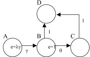
Figure 2. A Q-learning example. The values for

actions from A-B, B-D and C-D (γ, 1 and 1

respectively) have been previously learned for D as the goal location (reward 1). The value for action B-C is currently 0. The actions A-B and B-B-C have just

been performed giving eligibility traces of λγ and 1

respectively.

Watkins’ Q(λ) cuts off eligibility traces when a non-optimal action is chosen, for example when an

exploratory move is made. This is because it can not be guaranteed that the error for such an action is applicable to previous action choices as shown in Figure 2.

The error for action B-C in Figure 2 is γ, and the value of action B-C will correctly be trained towards this value. However, if an eligibility trace update were made for action A-B the value of this action would be trained too high. To avoid this problem, the eligibility traces for all state-action pairs, excluding the current state-action, to zero when a non-optimal action is taken. However, in our case non-optimal actions, with respect to each state, will be chosen very frequently and Watkins’ Q(λ) will perform little better than Q(0).

γ2

0

γ

e=1 e=λγ

1

A

B

C

[image:3.612.67.240.488.598.2]

D

Figure 3. A Q-learning example. The values for

actions from A-B, B-C and C-D (γ2, γ and 1) have

been previously learned for D as the goal location (reward 1). The value for action B-D is currently 0. The actions A-B and B-D have just been performed giving eligibility traces of λγ and 1 respectively.

To avoid this we make use of the triangular inequality to perform additional updates for all state-action pairs not updated using Watkins’ Q(λ). The error for action B-D in Figure 3 is 1 and using Watkins’ Q(λ) the value for this action will be trained towards this value. But since a non-optimal action has been chosen (0<γ) the value for action A-B will not be updated, and indeed the calculated error is too high for this action, the true error is γ-γ2_. Equation 3, the Q-value equivalent of the “triangular” inequality, correctly identifies this case.

QsC (sA,aA) ≥γ × Q sB (sA,aA) × Q sC (sB, aB) (3)

This equation can only be used to train the value

QsC(sA,aA) in the positive direction. However, if

q-values are initialised with some low value, and if the environment is reasonably deterministic, this is not a severe limitation and performance should be considerably better than Watkins’ Q(λ) alone.

time step as though the inverse action had just been performed from the current state to the previous state. This is particularly important for CQL since actions will frequently be moving away from the location for which values are being updated. The enhanced algorithm, including the “triangular” inequality and inverse updates is shown below:

Initialise Qs*(s,a) and es*(s,a)=0 for all s*,s,a

Initialise s, a Repeat:

Take action a, observe s′

Choose action a’ from s’ For all possible states s*: es*(s,a)Å1

δÅ rs* + γmaxa′Qs*(s′,a′) - Qs*(s,a)

for all state-action pairs s″, a″: if es*(s″,a″)>0

Q(λ) Update

Qs*(s″,a″) Å Qs*(s″,a″) +αδes*(s″,a″)

else

Triangular Inequality Update

δ″ÅγQs(s″,a″)[rs*+γmaxa Qs*(s′,a)]-Qs*(s″,a″) if δ″>0

Qs*(s″,a″) Å Qs*(s″,a″) + αδ″ Now update traces

if a′ = arg maxa Qs*(s,a) and s′≠s*

es*(s″,a″)Åγλes*(s″,a″) else

es*(s″,a″)Å0 Inverse Action Update

δ′ Å r′s* +γmaxa Qs*(s,a) - Qs*(s′,a-1)

Qs*(s′,a-1)Å Qs*(s′,a-1) +αδ′ sÅs′; aÅa′

where a-1 _{is the inverse of action a, e}

s*is the eligibility trace for s*, δ″ is the error resulting from “triangular” inequality updates and δ′ is the error resulting from inverse action updates. The reward for inverse actions,

r′s*, with respect to s* is 1 if s=s* and 0 otherwise. The value Qs*(s*,a) is defined to be 0 for all a.

Note that the CQL algorithm effectively learns a model of the environment and could be used for “planning” updates as described in Sutton and Barto[2]. Indeed, careful application of the “triangular” inequality could be used to devise more update rules for training and planning in both the forward and reverse directions. An additional refinement would be to replace the eligibility trace in Watkins’ Q(λ) updates with the Q-value from the location being considered to the current location.

2.1. Choosing an Action

Having learnt a ‘map’ of the environment, all that remains is to choose an appropriate action. That is, a state must be chosen as an ultimate goal.

To do this each location is assigned a value, V, initially set to Veq. At each time step, the value for the current location is updated to the experienced reward (in the maze task the reward will be 1 if the platform is reached and 0 otherwise). The value for all other locations decays back towards Veq.

The state with the highest expected reward, R, as calculated in equation 3, is chosen as the current goal. Once a goal location is chosen the ε-greedy action with respect to the goal is selected.

Rs* = Vs* × maxa Qs*(s,a) (3)

This technique gives a good balance between exploration and maximising reward, and could be applied to many reinforcement learning problems in conjunction with CQL.

The time complexity of the CQL algorithm is O(|S|2 _|A|). While this may be a limitation of the algorithm, Wierling and Schmidhuber have proposed a method of “Fast Online Q(λ)”[17] which has complexity O(|A|). If adapted to CQL this would reduce the complexity of the algorithm to O(|S||A|).

3.

The Simulation

[image:4.612.370.503.491.623.2]

The CQL method was tested for its ability to solve the RMW and DMP tasks as described in Steele and Morris [4]. Input to the learning system was via 400 simulated place cells, which is comparable to the number of place cells in Foster et al[3]. Unlike Foster and colleagues, the environment was discretised into 400 corresponding locations in a square 20×20 square grid (note that some locations are not reachable). Movement was restricted to the eight adjacent locations, with the action being performed in one time step.

The platform was the same size as a single place field making it proportionately the same size as in Steele and Morris[4]. Platform locations were chosen to minimize the possibility of straight-line movement between platform and start locations.

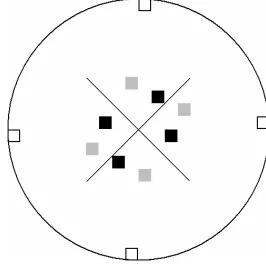
The system was also tested on the RMW and DMP tasks for a watermaze with a centrally located, cross-shaped obstacle as shown in Figure 4.

To improve the efficiency of searching when the platform location is unknown the system was given a slight preference for travelling in the same direction as chosen at the previous time step. This is similar to Foster and colleagues’ decision to add momentum to their system. In addition, non-greedy actions were limited to the two directions adjacent to the greedy action.

4.

Results

Tests were first carried out to compare the performance of non-concurrent Q(λ) and the CQL algorithm on the RMW task with no central barrier (Figure 5).

a)

0 50 100 150 200 250 300 350

1 2 3 4 5 6 7 8 9

Day

T

ime S

teps

Q CQL

b)

0 50 100 150 200 250 300 350

1 2 3 4 5 6 7 8 9

Day

T

ime S

teps

[image:5.612.59.283.340.712.2]

CQL-I CQL-TI

Figure 5. Performance of Watkin’s Q(λ) and

concurrent Q-learning on the RMW task (no

barrier). Q(λ) (labeled Q) and the basic CQL

algorithm (CQL) are shown in (a). CQL with inverse action updates (CQL-I), and CQL with inverse action and “triangular” inequality updates (CQL-TI) are shown in (b). λ=.95, γ=.90 in all cases.

Three versions of CQL were compared, the basic CQL algorithm (CQL), CQL with inverse action updates (CQL-I) and CQL with inverse action and “triangular inequality” updates (CQL-TI).

Like the actor-critic architecture in Foster et al[3], Q(λ) is able to learn the initial goal location quite quickly, but it still suffers the same limitations when the goal location changes, as expected. Any improved performance over actor-critic would be due to the inclusion of eligibility traces.

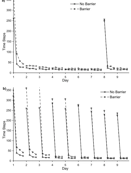
[image:5.612.324.547.367.662.2]

All versions of the CQL algorithm performed better than Q(λ) when the platform was moved, and also performed as well or better during the initial training. CQL-TI performed significantly better than CQL and CQL-I. It is also worth noting that, although a direct comparison is impossible, all CQL versions appear to perform better than the rat. This would suggest that it may take some time for place fields to stabilise in a new environment. Because place cells are idealised in this experiment, the CQL model has an advantage over the biological system. Figure 6 compares the performance of CQL-TI in the watermaze tasks for mazes with and without the central barrier.

a)

0 50 100 150 200 250 300 350

1 2 3 4 5 6 7 8 9

Day

T

ime S

teps

No Barrier Barrier

b)

0 50 100 150 200 250 300 350

1 2 3 4 5 6 7 8 9

Day

T

ime S

teps

No Barrier Barrier

Performance on the watermaze task is poorer when a barrier is included, but this is to be expected since optimal path lengths are longer. Despite the barrier the CQL algorithm is still able to achieve “one-trial” learning.

5.

Conclusion

The RL technique presented performed better than Watkins’ Q(λ) in a simulated Morris watermaze. Furthermore, unlike goal-dependant RL techniques, when the goal location was moved in the RMW and DMP tasks, no interference was evident, and “one-trial” learning was observed. This demonstrates that the observed behaviour of rats in these tasks does not require a coordinate mapping technique such as that proposed by Foster and colleagues. In addition, it was demonstrated that CQL is not unduly effected by the presence of barriers.

While CQL has been presented as a tool for autonomous mapping and navigation, the algorithm could be applied to any RL problem, especially problems where it is desirable or necessary for reward conditions to change. Not only does CQL experience no interference from previously learned goals, but is also able to apply all previous knowledge to the new problem.

Further work will examine the performance of the system under conditions requiring novelty detection and detour behaviour. The system will also be coupled with a learnt, continuous place cell system and further “triangular inequality” updates will be investigated for use in both training and planning.

Acknowledgements

We would like to thank Richard Dazeley for valuable discussions.

References

[1] R. S. Sutton, Learning to predict by the methods of temporal differences, Machine Learning, Vol. 3, pp. 9-44, 1988

[2] R. S. Sutton and A. G. Barto, Reinforcement Learning: An Introduction, MIT Press, 1998

[3] D. J. Foster, R. G. M. Morris and P. Dayan, A model of hippocampally dependent navigation, using the temporal difference learning rule, Hippocampus, Vol. 10, pp. 1-16, 2000

[4] R. J. Steele and R. G. M. Morris, Delay-dependent impairment of a matching-to-place task with chronic and intrahippocampal infusion of the NMDA-Antagonist D- AP5, Hippocampus, Vol. 9, pp. 118-136, 1999

[5] R. G. M. Morris, Spatial localization does not require the presence of local cues, Learning and Motivation, Vol. 12, pp. 239-260, 1981

[6] J. O'Keefe and J. Dostrovsky, The hippocampus as a spatial map. Preliminary evidence from the unit activity in the freely-moving rat., Brain Research, Vol. 34, pp. 171-175, 1971

[7] J. O'Keefe, Place units in the hippocampus of the freely moving rat, Experimental Neurology, Vol. 51, pp. 78-109, 1976

[8] R. U. Muller and J. L. Kubie, The firing of hippocampal place cells predicts the future position of freely moving rats, The Journal of Neuroscience, Vol. 9, pp. 4101-4110, 1989

[9] D. Joel, Y. Niv and E. Ruppin, Actor-critic models of the basal ganglia: new anatomical and computational perspectives, Neural Networks, Vol. 15, pp. 535-547, 2002

[10] W. Schultz, L. Tremblay and J. R. Hollerman, Reward processing in primate orbitofrontal cortex and basal ganglia, Cerebral Cortex, Vol. 10, pp. 272-283, 2000

[11] W. Schultz and A. Dickinson, Neuronal Coding of Prediction Errors, Annual Review of Neuroscience, Vol. 23, pp. 473-500, 2000

[12] A. G. Barto, R. S. Sutton and C. W. Anderson, Neuronlike adaptive elements that can solve difficult learning control problems, IEEE Transactions on Systems, Man, and Cybernetics, Vol. SMC-13, pp. 834-846, 1983

[13] G. A. Rummery and M. Niranjan, On-line q-learning using connectionist systems, Technical Report CUED/F-INFENG/TR 166, Cambridge University Engineering Department, 1994

[14] S. P. Singh and R. S. Sutton, Reinforcement learning with replacing eligibility traces, Machine Learning, Vol. 22, pp. 123-158, 1996

[15] C. Watkins and P. Dayan, Q-Learning, Machine Learning, Vol. 8, pp. 279-292, 1992

[16] J. Peng and R. J. Williams, Incremental multi-step Q-learning, Machine Learning, Vol. 22, pp. 283-290, 1996