A Unifying E2-Quasi Exactly Solvable Model

City, University of London Institutional Repository

Citation

: Fring, A. (2016). A Unifying E2-Quasi Exactly Solvable Model. Springer

Proceedings in Physics, pp. 235-248. doi: 10.1007/978-3-319-31356-6_15

This is the accepted version of the paper.

This version of the publication may differ from the final published

version.

Permanent repository link:

Link to published version

: http://dx.doi.org/10.1007/978-3-319-31356-6_15

Copyright and reuse:

City Research Online aims to make research

outputs of City, University of London available to a wider audience.

Copyright and Moral Rights remain with the author(s) and/or copyright

holders. URLs from City Research Online may be freely distributed and

linked to.

City Research Online: http://openaccess.city.ac.uk/ [email protected]

arXiv:1507.00611v1 [quant-ph] 2 Jul 2015

A unifying E2-quasi exactly solvable model

Andreas Fring

Department of Mathematics, City University London, Northampton Square, London EC1V 0HB, UK E-mail: [email protected]

Abstract: _{A new non-Hermitian E2-quasi-exactly solvable model is constructed}

con-taining two previously known models of this type as limits in one of its three parameters. We identify the optimal finite approximation to the double scaling limit to the complex Mathieu Hamiltonian. A detailed analysis of the vicinity of the exceptional points in the parameter space is provided by discussing the branch cut structures responsible for the chirality when exceptional points are surrounded and the structure of the corresponding energy eigenvalue loops stretching over several Riemann sheets. We compute the Stielt-jes measure and momentum functionals for the coefficient functions that are univariate weakly orthogonal polynomials in the energy obeying three-term recurrence relations.

1. Introduction

In addition to the interesting mathematical aspect of enlarging the set of sl2(C) [1, 2] to

E2-quasi-exactly solvable models [3], the latter type also constitutes the natural framework for various physical applications in optics where the formal analogy between the Helmholtz equation and the Schr¨odinger equation is exploited [4, 5, 6, 7, 8, 9, 10, 11, 12, 13]. Fur-thermore, a special case of these systems with a specific representation corresponds to the complex Mathieu equation that finds an interesting application in nonequilibrium statisti-cal mechanics, where it corresponds to the eigenvalue equation for the collision operator in a two-dimensional classical Lorentz gas [14, 15].

to obtain interesting information about the complex Mathieu system. On the other hand, for some applications it may also be sufficient to study an approximate behaviour for some finite values of the coupling constants. For that purpose we identify the parameter for which the general model is the optimal approximation for the complex Mathieu system.

Our manuscript is organized as follows: In section 2 we introduce the general unifying model involving three parameters. We determine the eigenfunctions by solving the stan-dard three-term recurrence relations for the coefficient functions and determine the energy eigenfunction from the requirement that the three-term recurrence relations reduce to a two-term relation. We devote section three to the study of the exceptional points and their vicinities in the parameter space. The explicit branch cut structure is provided that ex-plains the so-called energy eigenvalue loops. In section 4 we compute the central properties of the weakly orthogonal polynomials entering as coefficient functions in the Ansatz for the eigenfunctions, i.e. their norms, the corresponding Stieltjes measure and the momentum functionals. We state our conclusions in section 5.

2. A unifying E2-quasi-exactly solvable model

The general notion [1, 2] underlying solvable Hamiltonian systems is that its Hamiltonian operators H acting on some graded spaceVn as H:Vn 7→ Vn preserves the flag structure

V0 ⊂V1 ⊂ V2 ⊂. . .⊂Vn ⊂. . . A distinction is usually made between exactly and

quasi-exactly solvable, depending on whether the structure preservation holds for an infinite or a finite flag, respectively. Here we are concerned with the latter. Lie algebraic versions of Hamiltonians in this context are usually taken to be of sl2(C)-type [1, 2], but as recently proposed [3, 24], they may also be taken to be of a Euclidean Lie algebraic type, thus giving rise to qualitatively new structures.

At present two different types ofE2-quasi-exactly solvable models were identified

H(1)_E2 =J2+ζ2(u2−v2)2+ 2iζN(u2−v2), ζ, N ∈R_{, (2.1)}

H(0)_E2 =J2+ζuvJ + 2iζN(u2−v2), (2.2) in [3] and [24], respectively. Both Hamiltonians are expressed in terms of the E2-basis operatorsu,v and J that obey the commutation relations

[u, J] =iv, [v, J] =−iu, [u, v] = 0. (2.3)

Except for H(0)_E2 at N = 1/4, both Hamiltonians are non-Hermitian, but respect the anti-linear symmetry [25] PT3 : J → J, u → v, v → u, i → −i as defined in [10]. For the particular representation J := −i∂θ, u := sinθ v := cosθ the PT3-symmetry is simply

PT3:θ→π/2−θ,i→ −i, such that the invariant vector spaces over Rwere defined as

V_ns(φ₀) : = span

φ₀

sin(2θ), isin(4θ), . . . , in+1sin(2nθ)

θ∈R,PT₃(φ₀) =φ₀ ∈L ,(2.4)

V_nc(φ₀) : = span{φ₀[1, icos(2θ), . . . , incos(2nθ)]|θ∈R_{,PT3(φ0) =φ0∈L}. (2.5)}

more detail in [3]. The behaviour found allowed to identify the Hamiltonians H_E(1)₂ and

H(0)_E

2 in (2.1) and (2.2) as quasi-exactly solvable. The general structure suggests that there

might be a master Hamiltonian that unifies the above Hamiltonians into one preserving the quasi-exact solvability. We demonstrate here that this is possible and study the properties of that model.

Thus we introduce the new Hamiltonian

H(N, ζ, λ) =J2+ 2(1−λ)ζuvJ +λζ2(u2−v2)2+ 2iζN(u2−v2), λ, ζ, N ∈R_{, (2.6)}

and demonstrate explicitly that it is indeed E2-quasi-exactly solvable. First we observe thatH(N, ζ, λ) interpolates between the two models in (2.1) and (2.2) by varying λ, since

lim

λ→1H(N, ζ, λ) =H (1)

E2 and lim

λ→0H(2N, ζ/2, λ) =H (0)

E2. (2.7)

Furthermore,H(N, ζ, λ) reduces to the complex Mathieu Hamiltonian in the double scaling limit limN→∞,ζ→0H(N, ζ, λ) =HMat =J2+ 2ig(u2−v2) for g:=N ζ <∞. We also note thatH†_{(N, ζ, λ) =H(1−λ−N, ζ, λ), which implies thatH(N, ζ, λ) is non-Hermitian unless}

2N = 1−λ, with free coupling constant ζ ∈R_.

Given the structure for the vector spaces in (2.4) and (2.5) we now make the follow-ing Ans¨atze for the two fundamental solutions of the corresponding Schr¨odinger equation

HNψN =EψN

ψc_N(θ) =φ₀

∞

X

n=0

incnPn(E) cos(2nθ), and ψsN(θ) =φ0

∞

X

n=0

in+1cnQn(E) sin(2nθ), (2.8)

where the PT3-symmetric ground state is taken to be φ0 = e

i

2ζcos(2θ) and the constant

cn is cn = 1/ζn(N+λ)(1 +λ)n−1[(1 +N + 2λ)/(1 +λ)]n−1 with (a)n := Γ (a+n)/Γ (a)

denoting the Pochhammer symbol. The constants are chosen conveniently in order to ensure the simplicity of the to be determinedn-th and (n−1)-th order polynomialsPn(E),

Qn(E) in the energiesE, respectively. Upon substitution into the Schr¨odinger equation we

obtain the three-term recurrence relations

P2 = (E−λζ2−4)P1+2ζ2[N−1] [N+λ]P0, (2.9)

Pn+1 = (E−λζ2−4n2)Pn+ζ2[N +nλ+ (n−1)] [N −(n−1)λ−n]Pn−1, (2.10)

Q2 = (E−4−λζ2)Q1, (2.11)

Qm+1 = (E−λζ2−4m2)Qm+ζ2[N+mλ+ (m−1)] [N−(m−1)λ−m]Qm−1,(2.12)

for n = 0,2, . . . and for m = 2,3,4, . . . Note that a more generic Ansatz for the unifying model involving two independent coupling constantsµ,λin the termsµζuvJ+λζ2(u2−v2)2 leads to a four term recurrence relation in which the highest term is always proportional to

we obtain

P1 = E−λζ2, (2.13)

P2 = λ2ζ4+ 2ζ2[λ−λE+N(λ+N−1)] + (E−4)E,

P3 = −λ3ζ6+λζ4 λ(2λ+ 3E−13)−3N2−3(λ−1)N + 2

+ (E−16)(E−4)E

−ζ2

3λE2+E 2λ2−3N2−3λ(N+ 11) + 3N+ 2

+ 32(λ+N(λ+N −1))

,

and likewise withQ1 = 1 we compute

Q2 = E−4−λζ2, (2.14)

Q3 = λ2ζ4+ζ2

λ(15−2λ−2E) +N2+ (λ−1)N −2

+ (E−16)(E−4),

Q4 = −λ3ζ6+λζ4

8 +λ(8λ+ 3E−38)−2N2−2(λ−1)N

+ (E−36)(E−16)(E−4)

+ζ2

−8 −12λ2+ 69λ+ 5λN+ 5(N −1)N −12

+ζ2

−3λE2+ 2E (47−4λ)λ+N2+ (λ−1)N −4

.

In both cases we observe the typical feature for quasi-exactly solvable systems that the three term relation can be reset to a two-term relation at a certain level. This is due to the fact that in (2.10) and (2.12) the last term vanishes whenm=n= ˆn=−(1 +N)/(1 +λ) or m=n= ˜n= (λ+N)/(1 +λ). Thus when taking N = ˜n+ (˜n−1)λwe find the typical factorization

Pn˜+ℓ=Pn˜Rℓ and Q˜n+ℓ =Qn˜Rℓ. (2.15)

The first solutions for the factor Rℓ are easily found from (2.10) and (2.12) to

R1 = E−4˜n2−λζ2, (2.16)

R2 = (E−4˜n2−λζ2)(E−4(˜n+ 1)2−λζ2)−2˜n(1 +λ)2ζ2. (2.17)

Next we compute the energy eigenvalues En˜ from the constraints P˜n(E) = 0 and

Qn˜(E) = 0 for the lowest values of N. For the solutions related to the even fundamental solution in (2.8) we find

N = 1 : E₁c =λζ2, (2.18)

N = 2 +λ: E₂c,±= 2 +λζ2±2

q

1−(1 +λ)2_ζ2_{, (2.19)}

N = 3 + 2λ: E₃c,ℓ= 20 3 +λζ

2₊4 ˆΩ 3 e

iπℓ

3 +1

3

52−12(1 +λ)2ζ2

e−iπℓ3 Ωˆ−1, (2.20)

with ˆΩ3 _{:= 35 + 18(λ+ 1)}2_ζ2₊q

3(λ+ 1)2_ζ2₋₁₃3

+

18(λ+ 1)2_ζ2_{+ 35}2

,ℓ= 0,±2. For the solutions related to the odd fundamental solution in (2.8) we obtain

N = 2 +λ: E₂s= 4 +λζ2, (2.21)

N = 3 + 2λ: E₃s,±= 10 +ζ2λ±2

q

9−(λ+ 1)2_ζ2_{, (2.22)}

N = 4 + 3λ: E₄s,ℓ= 56 3 +λζ

2₊4Ω 3 e

iπℓ

3 +1

3

196−12(1 +λ)2ζ2

e−iπℓ3 Ω−1, (2.23)

with Ω3:= 143 + 18ζ2(λ+ 1)2+

q

3ζ2(λ+ 1)2₋₄₉3

+ 18ζ2(λ+ 1)2_{+ 143}2

3. Exceptional points and their vicinities

The special point in parameter space where two real energy eigenvalues viewed as functions of the coupling constants merge and subsequently split into a complex conjugate pair is usually referred to as exceptional point [26, 27, 28, 29]. In our system these points can be computed in an explicit simple and straightforward manner. Using that by definition the discriminant ∆ equals the product of the squares of the differences of all energy eigenvalues

Ei for 1≤ i ≤n, i.e. ∆ = Q_1≤i<j≤n(Ei −Ej)2 one obtains the exceptional points from

the real zeros of ∆(E). For practical purposes one may also exploit the fact [3], that the discriminant equals the determinant of the Sylvester matrix. This viewpoint has the advantage that it does not require the computation of all the eigenvalues and is more efficient when the sole purpose is to find the exceptional points. Thus in our case we have to find the real zeros of the discriminants ∆c

˜

nand ∆sn˜for the polynomialsP˜n(E) andQn˜(E), respectively. Extracting overall constant factors κ as ∆ =κ∆, that do not contribute to˜ the zeros, we obtain for the lowest values of ˜n

˜

∆c₂ = ˆζ2−1, (3.1)

˜

∆s₃ = ˆζ2−9,

˜

∆c₃ = ˆζ6−ˆζ4+ 103ˆζ2−36,

˜ ∆s

4 = ˆζ 6

−37ˆζ4+ 991ˆζ2−3600,

˜

∆c₄ = ˆζ12+ 2ˆζ10+ 385ˆζ8−33120ˆζ6+ 16128ˆζ4−732276ˆζ2+ 129600,

˜

∆s₅ = ˆζ12−94ˆζ10+ 7041ˆζ8−381600ˆζ6+ 6645600ˆζ4−78318900ˆζ2+ 158760000,

where we abbreviated ˆζ :=ζ(1 +λ).

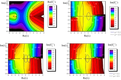
There exist many detailed studies about the structures in the coupling constant space in the vicinity of the exceptional points [30, 31, 32, 33, 34]. It is evident that when tracing a complex energy eigenvalue E as functions of the coupling constants, λ or ζ in our case, the corresponding path in the energy plane will inevitably pass through various Riemann sheets due to the branch cut structure. As a consequence one naturally generates eigenvalue loops that stretch over several Riemann sheets. This phenomenon is well studied for a large number of models and we demonstrate here that it also occurs in quasi-exactly solvable models. The basic principle can be demonstrated with the square root singularity occurring in E₂c,± with branch cuts from (−∞,−1−1/ζ) and (1/ζ −1,∞). The energy loops are generated by computing E₂c,±(λ = ˜λ+ρeiπφ_{, ζ) for some fixed values of ζ, center ˜λ and}

the radiusρ in the λ-plane as functions ofφas illustrated in figure 1(a) and (b). In panel (a) we simply trace the energy around a point in parameter space that leads to two real eigenvalues. For a small radius ones reaches the starting point by encircling ˜λjust once. However, when the radius is increased one needs to surround ˜λtwice to reach the starting point and when the radius is increased even further one only needs to surround ˜λ once switching, however, between both energy eigenvalues.

-4 -2 0 2 4 6 8 -8 -6 -4 -2 0 2 4 6 8 2 2 1 1 0 0 4 3 2 1 0 2 0 2 0 (a) +, -, +, -, +, -, Im(E) Re(E)

-6 -4 -2 0 2 4 6 8 10 12 -12 -8 -4 0 4 8 12 2 3 2 1 1 1 (b) +, -, +, -, +, -, Im(E) Re(E) 2 0 2 0 4 0 4 0

Figure 1: Energy eigenvalue loopsE2c,±(˜λ+ρe

iπφ_{, ζ) around two real eigenvalues panel (a) and}

around an exceptional point panel (b) as functions ofφ, indicated by the numbers on the loops, for fixed value ofζ = 1/2 at ˜λ= 1/10 in (a) and ˜λ= 1 in (b). The energy eigenvalues forρ= 0 are distinct in panel (a) asE2c,−= 0.35,E

c,+

2 = 3.70 and coalesce to an exceptional point in panel (b) asE2c,−=E

c,+ 2 = 9/4.

-1.0 0.0 1.0 2.0 0.0 -1.0 1.0

-5 -4 -3 -2 -1 0 1 2 3 4 5 -2.0 -1.5 -1.0 -0.5 0.0 0.5 1.0 1.5 2.0 Re(E c,-2 ) C2 Re( ) Im( ) -1.0 -0.50 0.0 0.50 1.0 1.5 2.0 2.5 3.0

3.02.01.0

-1.0 1.0 0.0 0.0 -2.0 2.0 -3.0 3.0 -1.0 -4.0 -2.0 -5.0 5.0 -3.0

-5 -4 -3 -2 -1 0 1 2 3 4 5 -2.0 -1.5 -1.0 -0.5 0.0 0.5 1.0 1.5 2.0 = 0.5 = 2.5 Im(E c,-2 ) Re( ) Im( ) -5.0 -4.0 -3.0 -2.0 -1.0 0.0 1.0 2.0 3.0 4.0 5.0 -3.0 -2.0 -1.0 0.0 0.0 0.0 1.0 -1.0 2.0 -2.0 1.0 3.0 -3.0 2.0 4.0 -4.0 3.0 -5.0

-5 -4 -3 -2 -1 0 1 2 3 4 5 -2.0 -1.5 -1.0 -0.5 0.0 0.5 1.0 1.5 2.0 Im(E c,+ 2 ) Re( ) Im( ) -5.0 -4.0 -3.0 -2.0 -1.0 0.0 1.0 2.0 3.0 4.0 5.0 -3.0 -2.0 -1.0 0.0 0.0 0.0 1.0 -1.0 2.0 -2.0 1.0 3.0 -3.0 2.0 4.0 -4.0 3.0 -5.0

-5 -4 -3 -2 -1 0 1 2 3 4 5 -2.0 -1.5 -1.0 -0.5 0.0 0.5 1.0 1.5 2.0 = 0.5 = 2.5 Im(E c,+ 2 ) Re( ) Im( ) -5.0 -4.0 -3.0 -2.0 -1.0 0.0 1.0 2.0 3.0 4.0 5.0

Figure 2: Energy levels and branch cut structure forE2c,±for fixedζ= 1/2 as functions ofλ. The branch cuts extend to the left and right from the exceptional points (−∞,−3) and (1,∞).

This structure is the same for intermediate radii. For large radii we cross the first cut already at a half circle turn, such that one returns back to the original value already after one complete turn.

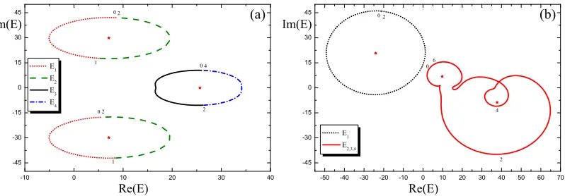
When more eigenvalues are present the structure will be more intricate. Considering for instance a scenario with four eigenvalues in the form of two complex conjugate eigenvalues and an exceptional point, see figure 3(a), we need to perform again at least two turns in theλ-plane in order to return to the initial position for the energy loops when surrounding an exceptional point. The two complex conjugate eigenvalues may be enclosed with just one turn, albeit we require again different energy eigenvalues for this. When enlarging the radius the loops will eventually merge as depicted in figure 3(b) for a situation with a degenerate complex eigenvalue and two complex eigenvalues. We observe that for the given values we have to surround the chosen point at least three times to obtain a closed energy loop surrounding the indicated centers.

-10 0 10 20 30 40 -45

-30 -15 0 15 30 45

4 2

2

2

1 1

0

0 0

(a)

E 1 E 2 E 3 E 4

Im(E)

Re(E)

-50 -40 -30 -20 -10 0 10 20 30 40 50 60 70 -45

-30 -15 0 15 30 45

2 6

0 2

4 0

(b)

E 1 E 2,3,4

Im(E)

Re(E)

Figure 3: Energy eigenvaluesEc

4(˜λ+ρeiπφ, ζ) as functions ofφ, indicated by the numbers on the loops, for fixed value ζ = 1/2 at ˜λ= 9.5284 in (a) and ˜λ= 5.2562 +i9.9526 in (b). The energy eigenvalues forρ= 0 in panel (a) are E4c,1 =E

c,2

4 = 25.6613, E c,3 4 = (E

c,4 4 )

∗

= 7.1029 +i29.8106 andE4c,1=E

c,2

4 = 37.7449−i8.7611,E c,3

4 = 9.8103 +i6.7668,E c,4

4 =−24.0439 +i20.7081 in panel (b). The radii areρ= 4.0 andρ= 8.5 in panel (a) and (b), respectively.

In the same manner as for the simpler scenario one may understand the nature of these loops from an analysis of the branch cut structure of the energy as seen in figure 4. Tracing the indicated radii at ρ= 4.0 andρ= 8.5 in figure 4 produces the energy loops in figure 3 when properly taking care of the analytic continuation at the branch cuts.

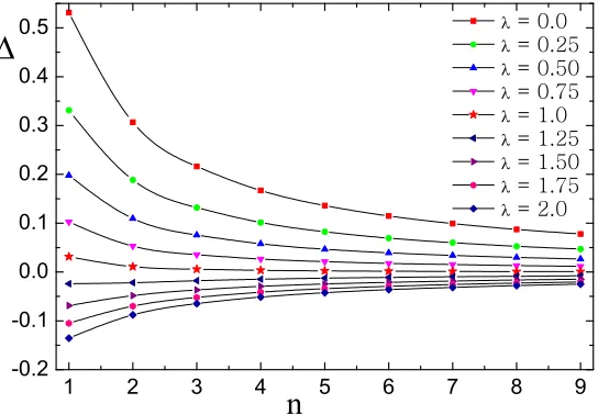
Comparing the rate of the approach for different values ofλwe conclude thatH(N, ζ, λ= 1) is the best approximation to the complex Mathieu system for some finite values of N.

-25 -20 -15 -10 -5.0 -5.0 -10 -15 0.0 -20 0.0 5.0 -25

-15 -10 -5 0 5 10 15 -10 -8 -6 -4 -2 0 2 4 6 8 10 Re(E c,1 4 ) Re( ) Im( ) -25 -20 -15 -10 -5.0 0.0 5.0 10 35 30 25 20 15 10 5.0 0.0 5.0 0.0 -5.0 10 -5.0 -10 15 -10 -15 20 -20 -15 25 -25 -20 30 -30 -25 35 -35 -30 -40 -35 -45

-15 -10 -5 0 5 10 15 -10 -8 -6 -4 -2 0 2 4 6 8 10 Im(E c,1 4 ) Re( ) Im( ) -50 -45 -40 -35 -30 -25 -20 -15 -10 -5.0 0.0 5.0 10 15 20 25 30 35 40 45 50 30 25 20 15 10 10 10 15 15 10 20 20 25 25 15 5.0 30 30 20 25 35 35 30 35 35

-15 -10 -5 0 5 10 15 -10 -8 -6 -4 -2 0 2 4 6 8 10 Re(E c,2 4 ) Re( ) Im( ) 5.0 10 15 20 25 30 35 40 10 -15 -20 15 -25 -15 20 -30 -20 -25 -35 -30 -40 -35 -40

-15 -10 -5 0 5 10 15 -10 -8 -6 -4 -2 0 2 4 6 8 10 Im(E c,2 4 ) Re( ) Im( ) -40 -35 -30 -25 -20 -15 -10 -5.0 0.0 5.0 10 15 20 25 30 35 40 10 15 20 20 20 25 25 15 15 10 15 25 30 30 30 30 20

-15 -10 -5 0 5 10 15 -10 -8 -6 -4 -2 0 2 4 6 8 10 Re(E c,3 4 ) Re( ) Im( ) 5.0 10 15 20 25 30 35 5.0 0.0 0.0 5.0 -5.0 0.0 0.0 -5.0 10 -10 5.0 -5.0 5.0 -5.0 -10 10 -10 10 15 -15 -15 15

-15 -10 -5 0 5 10 15 -10 -8 -6 -4 -2 0 2 4 6 8 10 Im(E c,3 4 ) Re( ) Im( ) -15 -10 -5.0 0.0 5.0 10 15 20 35 35 30 30 25 40 40 30 30 25 25 25 25 20 20 20 20 20 15 15 35 35 30 30

-15 -10 -5 0 5 10 15 -10 -8 -6 -4 -2 0 2 4 6 8 10 Re(E c,4 4 ) Re( ) Im( ) 15 20 25 30 35 40 45 -35 -30 -25 -20 -15 15 -15 20 -20 -25 -30 -40 -15 -25

-15 -10 -5 0 5 10 15 -10 -8 -6 -4 -2 0 2 4 6 8 10 Im(E c,4 4 ) Re( ) Im( ) -40 -35 -30 -25 -20 -15 -10 -5.0 0.0 5.0 10 15 20 25 30 35 40

If one is exclusively interested in the computation of the exceptional point it is most efficient to carry out the double scaling limit already for the three-term relation (2.10) and (2.12) as explained in [3, 24].

1 2 3 4 5 6 7 8 9

-0.2 -0.1 0.0 0.1 0.2 0.3 0.4 0.5

= 0.0

= 0.25

= 0.50

= 0.75

= 1.0

= 1.25

= 1.50

= 1.75

= 2.0

n

Figure 5: Double scaling limit of limN→∞,ζ→0H(N, ζ, λ) =HMatto the smallest exceptional point atζM = 1.46877 with ∆(n) =ζ0N(n)−ζM,N(n) = (n+ 1) +nλforn= 1,2,3, . . ..

4. Weakly orthogonal polynomials

It is well known from Favard’s theorem [35, 36] that polynomials Φn(E) constructed from

three-term relations in the way mentioned above possess a normNΦ

n

L(ΦnΦm) =NnΦδnm. (4.1)

defined by the action of a linear functional L acting on arbitrary polynomialsp inE as

L(p) =

Z ∞

−∞

p(E)ω(E)dE, L(1) = 1. (4.2)

This norm may be computed in two alternative ways. The simplest way is to multiply the three-term relation by Φn−1 and act subsequently on the resulting equation with L. Using the property N_nΦ = L(Φ2_n) = L(EΦn−1Φn) together with (4.1) then simply yields

N_nΦ = Qn

k=1bk, where the bk are the negative coefficients in front of Φn−1. Whereas the first method simply assumes that the functional exist the second method goes further and actually provides an explicit expressions for the measure. As argued in [37] the concrete formulae forω(E) may be computed from

ω(E) =

ℓ

X

k=1

where the energies Ek are theℓ roots of the polynomial Φ(E). Theℓ constantsωk can be

determined by theℓ equations

ℓ

X

k=1

ωkΦn(Ek) =δn0, forn∈N0. (4.4)

In our case the integer ℓ are determined fromN =ℓ+ (ℓ−1)λand N = (ℓ+ 1) +ℓλ for thePℓ(E) and Qℓ+1(E), respectively.

Using the first method we obtain

N_nP = 2ζ2n(1 +λ)2n

1−N

1 +λ

n

λ+N

1 +λ

n

, n= 1,2,3, ... (4.5)

NQ

n =

1

2(N +λ)(1−N)N

P

n, n= 2,3,4, ... (4.6)

withNP

0 =N

Q

1 = 1. Due to the non-Hermitian nature of the Hamiltonian this norm is in general not positive definite. For instance for N = 4 + 3λwe have

N₀P = 1, N₁P =−24ζ2(1 +λ)2, N₂P = 240ζ4(1 +λ)4, N₃P =−1440ζ6(1 +λ)6. (4.7)

The exception is the class of models where the Hamiltonian becomes Hermitian, i.e. when

λ= 1−2N holds. For this value of λ the expressions in (4.5) and (4.6) become positive definite

N_nP = 21+2nζ2n(N −1)2n

1 2

2

n

= 2ζ2(N−1)2N_nQ. (4.8)

Let us now consider the second method and compute explicitly the measure for a few examples. For N = 2 +λ and N = 3 + 2λ we solve (4.4) for the even and odd solutions, respectively, to

ωc_± = 1 2±

1

2

q

1−(1 +λ)2_ζ2, and ω

s ±=

1 2 ±

3

2

q

9−(1 +λ)2_ζ2. (4.9)

Computing now (4.1) with (4.2) agrees with (4.5) and (4.6)

NP

0 = L(P02) =ωc++ωc−= 1 (4.10)

NP

1 = L(P12) =ωc+

E₂c,+−λζ22+ωc −

E₂c,−−λζ22=−4ˆζ2, (4.11)

N₂Q = L(Q2₂) =ωs₊E₃s,+−4−λζ22+ωs₋E₃s,−−4−λζ22 =−4ˆζ2. (4.12)

Similarly we compute forN = 3 + 2λ

ωc₁ = 1 3 −

260−60ˆζ2Ω +3ˆζ2+ 4Ω2+ 20Ω3

12

13−3ˆζ22+13−3ˆζ2Ω2_{+ Ω}4

, ω

c

2 =χ−2, ωc3=χ2, (4.13)

χ_ℓ = 1 3 +

3ˆζ2−20Ω + 4 1 + 2eiπℓ3

36(3ˆζ2+ Ω2₋₁₃₎ +

4 + 3ˆζ2−20eiπℓ3 Ω

121 + 2eiπℓ3 3ˆζ

2

−13+1−eiπℓ3

and confirm that

N₀P = L(P₀2) =ω₁c +ωc₂+ωc₃ = 1, (4.14)

N₁P = L(P₁2) =ω₁cP₁2(E₃c,0) +ωc₂P₁2(E₃c,−2) +ωc₃P₁2(E₃c,2) =−12ˆζ2,

N₂P = L(P₂2) =ωc₁P₂2(E₃c,0) +ω₂cP₂2(E₃c,−2) +ω₃cP₂2(E₃c,2) = 48ˆζ4

L(P1P2) = ωc1P1(E3c,0)P2(E3c,0) +ωc2P1(E3c,−2)P2(E3c,−2) +ωc3P1(E3c,2)P2(E3c,2) = 0.

Note that the last relation in (4.14) does not follow from the first method.

As the final quantity we also compute the moment functionals defined in [35, 36] as

µ_n:=L(En) =

ℓ

X

k=1

ωkEkn= n−1

X

k=0

ν(_kn)µ_k, (4.15)

Once again also these quantities can be obtained in two alternative ways, that is either from the computation of the integrals or directly from the original polynomialsPnandQn

without the knowledge of the constants ωk. In the last equation the coefficients ν(_kn) are

defined through the expansionPn(E) = 2n−1En−Pn−k=01ν (n)

k Ek andQn(E) = 2n−1En−1−

Pn−2

k=0ν (n)

k Ek for our even and odd solutions, respectively. For the even solutions with

N = 2 +λwe obtain

µP₀ = 1, (4.16)

µP₁ =λζ2, (4.17)

µP

2 =λ2ζ4−4ˆζ 2

, (4.18)

µP₃ =λ3ζ6−12λζ2ˆζ2−16ˆζ2, (4.19)

µP₄ =λ4ζ8−24λ2ζ4ˆζ2+ 16 ζ2−12

ζ4−64ˆζ2, (4.20)

and similarly for the odd solutions with N = 3 + 2λwe compute for instance

µQ₀ = 1, (4.21)

µQ₁ = 4 +λζ2, (4.22)

µQ₂ = 16−4ˆζ2+λ2ζ4, (4.23)

µQ₃ =λ3ζ6−12 λ3+λ2+λ

ζ4−48(2λ2+ 3λ+ 2)ζ2+ 64. (4.24)

ThusH(N, ζ, λ) possesses indeed all the standard features of a quasi-exactly solvable model ofE2-type.

5. Conclusions

the complex Mathieu equation, we found that for λ = 1, i.e. H(1)_E2, finite values for N

best approximate the complex Mathieu system and mimic its qualitative behaviour. We provided a detailed discussion of the determination of the exceptional points and the en-ergy branch cut structure responsible for the intricate enen-ergy loop structure stretching over several Riemann sheets. The coefficient functions are shown to possess the standard properties of weakly orthogonal polynomials.

Acknowledgments: I am grateful to Kazuki Kanki for making reference [15] available to me.

References

[1] A. V. Turbiner, Quasi-Exactly-Solvable problems and sl(2) Algebra, Commun. Math. Phys. 118, 467–474 (1988).

[2] A. Turbiner, Lie algebras and linear operators with invariant subspaces, Lie Algebras, Cohomologies and New Findings in Quantum Mechanics, Contemp. Math. AMS, (eds N. Kamran and P.J. Olver)160, 263–310 (1994).

[3] A. Fring, E2-quasi-exact solvability for non-Hermitian models, J. Phys. A48, 145301(19) (2015).

[4] Z. H. Musslimani, K. G. Makris, R. El-Ganainy, and D. N. Christodoulides, Optical Solitons in PT Periodic Potentials, Phys. Rev. Lett.100, 030402 (2008).

[5] K. G. Makris, R. El-Ganainy, D. N. Christodoulides, and Z. H. Musslimani, PT-symmetric optical lattices, Phys. Rev.A81, 063807(10) (2010).

[6] A. Guo, G. J. Salamo, D. Duchesne, R. Morandotti, M. Volatier-Ravat, V. Aimez, G. A. Siviloglou, and D. Christodoulides, Observation of PT-Symmetry Breaking in Complex Optical Potentials, Phys. Rev. Lett. 103, 093902(4) (2009).

[7] B. Midya, B. Roy, and R. Roychoudhury, A note on the PT invariant potential 4cos2_{x+ 4iV}

0sin2x, Phys. Lett.A374, 2605–2607 (2010).

[8] H. Jones, Use of equivalent Hermitian Hamiltonian for PT-symmetric sinusoidal optical lattices, J. Phys. A44, 345302 (2011).

[9] E. Graefe and H. Jones, PT-symmetric sinusoidal optical lattices at the symmetry-breaking threshold, Phys. Rev. A84, 013818(8) (2011).

[10] S. Dey, A. Fring, and T. Mathanaranjan, Non-Hermitian systems of Euclidean Lie algebraic type with real eigenvalue spectra, Annals of Physics346, 28–41 (2014).

[11] S. Dey, A. Fring, and T. Mathanaranjan, Spontaneous PT-symmetry breaking for systems of noncommutative Euclidean Lie algebraic type, arXiv:1407.8097, to appear in Int. J. Theor. Phys.

[12] S. Longhi and G. Della Valle, Invisible defects in complex crystals, Annals of Physics334, 35–46 (2013).

[14] K. Kanki, Spontaneous breaking of a PT-symmetry in the Liouvillian dynamics at a nonhermitian degeneracy point, talk at the 15th International Workshop on

Pseudo-Hermitian Hamiltonians in Quantum Physics, May 18-23, University of Palermo, Italy (2015).

[15] Z. Zhang, Irreversibility and extended formulation of classical and quantum nonintegrable dynamics, PhD Thesis, The University of Texas at Austin (1995).

[16] A. Khare and B. P. Mandal, A PT-invariant potential with complex QES eigenvalues, Phys. Lett. A272, 53–56 (2000).

[17] B. Bagchi, S. Mallik, C. Quesne, and R. Roychoudhury, A PT-symmetric QES partner to the Khare–Mandal potential with real eigenvalues, Phys. Lett. A289, 34–38 (2001).

[18] C. M. Bender and M. Monou, New quasi-exactly solvable sextic polynomial potentials, J. Phys. A 38, 2179–2187 (2005).

[19] B. Bagchi, C. Quesne, and R. Roychoudhury, A complex periodic QES potential and exceptional points, J. Phys. A 41, 022001 (2008).

[20] F. G. Scholtz, H. B. Geyer, and F. Hahne, Quasi-Hermitian Operators in Quantum Mechanics and the Variational Principle, Ann. Phys.213, 74–101 (1992).

[21] C. M. Bender and S. Boettcher, Real Spectra in Non-Hermitian Hamiltonians Having PT Symmetry, Phys. Rev. Lett. 80, 5243–5246 (1998).

[22] C. M. Bender, Making sense of non-Hermitian Hamiltonians, Rept. Prog. Phys.70, 947–1018 (2007).

[23] A. Mostafazadeh, Pseudo-Hermitian Representation of Quantum Mechanics, Int. J. Geom. Meth. Mod. Phys.7, 1191–1306 (2010).

[24] A. Fring, A new non-Hermitian E2-quasi-exactly solvable model, Phys. Lett.379, 873–876 (2015).

[25] E. Wigner, Normal form of antiunitary operators, J. Math. Phys.1, 409–413 (1960).

[26] T. Kato, Perturbation Theory for Linear Operators, (Springer, Berlin) (1966).

[27] W. D. Heiss, Repulsion of resonance states and exceptional points, Phys. Rev. E61, 929–932 (2000).

[28] I. Rotter, Exceptional points and double poles of theS matrix, Phys. Rev. E67, 026204 (2003).

[29] U. G¨unther, I. Rotter, and B. F. Samsonov, Projective Hilbert space structures at exceptional points, Journal of Physics A: Mathematical and Theoretical 40, 8815 (2007).

[30] W. D. Heiss and H. Harney, The chirality of exceptional points, The European Physical Journal D - Atomic, Molecular, Optical and Plasma Physics17, 149–151 (2001).

[31] H. Mehri-Dehnavi and A. Mostafazadeh, Geometric phase for non-Hermitian Hamiltonians and its holonomy interpretation, Journal of Mathematical Physics49, 082105 (2008).

[32] I. Rotter, A non-Hermitian Hamilton operator and the physics of open quantum systems, Journal of Physics A: Mathematical and Theoretical 42, 153001 (2009).

[34] W. D. Heiss and G. Wunner, Fano-Feshbach resonances in two-channel scattering around exceptional points, The European Physical Journal D68(2014) 284.

[35] J. Favard, Sur les polynomes de Tchebicheff., C. R. Acad. Sci., Paris200, 2052–2053 (1935).

[36] F. Finkel, A. Gonzalez-Lopez, and M. A. Rodriguez, Quasiexactly solvable potentials on the line and orthogonal polynomials, J. Math. Phys. 37, 3954–3972 (1996).