An Optimization-based approach for vaccine prioritization

(1)

Rochester Institute of Technology

RIT Scholar Works

Theses Thesis/Dissertation Collections

8-19-2013

An Optimization-based approach for vaccine

prioritization

Timothy Schmoke

Follow this and additional works at:http://scholarworks.rit.edu/theses

This Thesis is brought to you for free and open access by the Thesis/Dissertation Collections at RIT Scholar Works. It has been accepted for inclusion in Theses by an authorized administrator of RIT Scholar Works. For more information, please [email protected].

Recommended Citation

(2)

R

.

I

.

T

An Optimization-Based Approach for Vaccine

Prioritization

by

Timothy J. Schmoke

A Thesis Submitted in Partial Fulfillment of the Requirements for the Degree of Master of Science in Industrial Engineering

Department of Industrial and Systems Engineering Kate Gleason College of Engineering

Rochester Institute of Technology

Rochester, NY

(3)

An Optimization-Based Approach for Vaccine Prioritization

Thesis

Advisor: Dr. Rubén A. Proaño

By: Timothy J. Schmoke (2013)

Committee Members:

Dr. Rubén A. Proaño

Assistant Professor, Industrial and Systems Engineering

Dr. Brian K. Thorn

Associate Professor, Industrial and Systems Engineering

Approved By:

(4)

1

Abstract

An effective vaccine prioritization process is essential to prevent the many issues that currently weaken global vaccination efforts. Identifying challenges associated with vaccine development is important when considering which initiatives will provide immunization that is effective, affordable, and easy to administer. The process of establishing priorities for vaccine development is complicated, though, by the conflicting interests of multiple stakeholders

involved in the vaccine market. Additionally, uncertainties exist regarding: (1) the resources and time required for vaccine development, (2) the expected benefits of development, and (3) the anticipated demand for vaccination, further complicating the prioritization process.

This study proposes a decision-support tool for prioritizing vaccine initiatives through the use of mathematical optimization models. The tool will allow a panel of decision makers to assess vaccine candidates over multiple criteria with information that is both quantitative and qualitative. This assessment will be the result of a methodology that integrates Data

Envelopment Analysis and the Analytic Hierarchy Process. Ultimately, the decision-support tool will allow researchers and funding agencies to determine which vaccine initiatives should be: more effective, affordable, profitable, reliable, easier to use and store, and more suitable to the needs of multiple populations from diverse locations and having multiple logistic needs.

1. Introduction

(5)

2

strategies for new vaccine development is timely and critical. This is evident in the 2010 National Vaccine Plan, a report by the U.S. government with goals for enhancing all aspects of vaccines and vaccination. In the report, strategies are listed to guide disease prevention and improve vaccination, including: “develop and implement a process for prioritizing and evaluating new vaccine targets of domestic and global public health importance” [1]. The Institute of Medicine (IOM) has also targeted vaccine prioritization as an integral part in the design of a national and global vaccine development strategy. Despite a few efforts by the IOM to address the vaccine prioritization problem, to date, no universally accepted method or model exists to guide these important decisions [2].

Prioritizing vaccine initiatives can provide a framework for organizations or stakeholders

in the vaccine market to discuss investment alternatives and converge toward solutions that

satisfy most parties. Additionally, allocating proper resources to a vaccine initiative can reduce

the time it spends in development, allowing it to provide immunization to the public sooner.

Increased interests, efforts, and collaborations related to vaccine-preventable diseases are adding

to the need for vaccine prioritization. Figure 1 shows the market attractiveness of vaccine

investments over the last 30 years. A renewed interest in vaccine development is evident, with a

(6)

3

Figure 1: Historical attractiveness of vaccine investments. SOURCE: Institute of Medicine, 2012 [2].

For any organization choosing to invest in the development of a vaccine initiative, there are a number of factors that make the decision to select one project over another challenging. Varying public health environments, social and economic infrastructures, political conditions, and climates, for example, can have a significant impact on the effectiveness and profitability of an initiative. These circumstances can vary significantly around the world and can heavily influence a vaccine initiative’s likelihood of success. Additionally, decision makers can face uncertainty regarding: the expected length of time for the vaccine to become licensed for use, the vaccine initiative’s financial viability, and the logistic challenges associated with vaccine

(7)

4

potential to cause epidemics and pandemics, whether the vaccine has characteristics that are

attractive for use in developing countries, and the cost-effectiveness of the vaccine [3].

Key stakeholders of the vaccine market assess the importance of vaccine criteria

differently, and while organizations’ internal mechanisms to set priorities are not well known or

publicized, information has been gathered about the varying priorities of the public sector,

private sector, and non-governmental groups. Manufacturers, for example, favor the

development of vaccines that promise high returns and involve the use of currently available

technologies. Non-governmental organizations such as UNICEF, GAVI, and PAHO, on the

other hand, are interested in expanding immunization in developing countries and developing

vaccines that are inexpensive, easy to distribute, and do not require the use of expensive cold

chains. Furthermore, different governments (from developing and industrialized nations) are

interested in the development of vaccines that target diseases specific to their regions.

An effective vaccine prioritization process will bring together government agencies,

vaccine manufacturers, humanitarian groups, and other organizations invested in the

development of vaccines, allowing them to collectively identify vaccine priorities that best

represent everyone’s interests or provide the least level of conflict. In this thesis, the

development of an optimization based heuristic is proposed that considers the interests of

multiple stakeholders to prioritize vaccine candidates that are at different developmental stages

and target different diseases. Moreover, a heterogeneous group of decision makers is assumed

with different interests and levels of expertise. Therefore, vaccine prioritization is addressed as a

multiple criteria decision making (MCDM) problem, involving multiple decision makers who

(8)

5

2. Previous Vaccine Prioritization Efforts

The Institute of Medicine, aware of the difficulty associated with vaccine prioritization, established three committees over the last 30 years to address the vaccine prioritization problem. In 1985, the Institute of Medicine (IOM) published its first report on vaccine prioritization: “New Vaccine Development: Establishing Priorities: Volume 1, Diseases of Importance in the United States” [4]. Part one of a two-part study, this report aimed to help the National Institute of Allergy and Infectious Diseases (NIAID) establish priorities for accelerated vaccine

development. The committee behind the report was charged with developing a decision-making framework to prioritize vaccine candidates for the US population. In addition, the committee was asked to evaluate the model’s ability to set priorities for vaccines needed by technologically less developed nations, and modify the model to rank potential vaccines for international use. The committee’s findings relative to the international aspects of vaccine development appeared in part two of the study: “New Vaccine Development: Establishing Priorities: Volume 2, Diseases of Importance in Developing Countries” [5].

The method used by the committee to rank vaccine initiatives was based on a quantitative model in which vaccine candidates were ranked according to two criteria: (1) expected health benefits measured by the reduction of morbidity and mortality, and (2) expected net savings of health care resources. A measurement system based on infant mortality equivalents (IMEs)1 was used to compare the health impacts of a disease versus the potential benefits of a vaccine. Estimates and judgments by experts were also used when information was incomplete. The

(9)

6

committee adopted a flexible format so that new candidate vaccines could be assessed similarly or current candidate vaccines could be reassessed with new data.

Since the time the report was published, analytical techniques have advanced and other metrics have proven to be better measures of health valuation. In addition, the epidemiological data used to compare diseases was variable in quality and in some cases, completely absent. This created a serious impediment to the development of a comprehensive prioritization scheme, leading the IOM to create a second committee in 2000 to address the same problem.

The 2000 report, “Vaccines for the 21st Century” [6], used an efficiency measure for deriving its priorities based on the incremental cost per incremental quality adjusted life year gained by vaccination ($/QALY). Using this measure, initiatives were grouped into one of four categories. The highest priority, Level I, was designated for vaccine programs projected to save money and increase the number of QALYs. Vaccine programs that did not save money were grouped into the remaining three categories based on the efficiency of the investment. Level II included candidates whose $/QALY was less than $10,000, Level III included candidates for which $/QALY ranged between $10,000 and $100,000, and Level IV was for candidates whose $/QALY was greater than $100,000.

(10)

7

The IOM’s most recent attempt at addressing the vaccine prioritization problem is currently in development and is the focus of the report: “Ranking Vaccines: A Prioritization Framework: Phase I: Demonstration of Concept and a Software Blueprint” [2]. For this recent modeling strategy, the committee limited its scope to models that consider multiple attributes; the committee recognized that the narrow range of attributes used to prioritize vaccines in the previous IOM studies significantly limited their value and applications. The three multi-attribute approaches that the committee reviewed were: mathematical programming, multi-attribute utility theory, and the analytic hierarchy process. These approaches were evaluated against four criteria: transparency, axiomatic foundation, priority scaling, and sensitivity analysis. Ultimately, multi-attribute utility theory was chosen for the foundation of the committee's work because it provides weights and data that are available for all users to see and use, independence from irrelevant alternatives (IIA), scaling that can be used for an ordinal ranking, and the ability to conduct sensitivity analyses on results [2].

The current committee's model improves upon the previous two by including multiple attributes that address the varied interests of the public sector, private sector, and

(11)

8

them. The prioritization model, in accompaniment with stakeholder input, should be able to generate a vaccine ranking that best addresses the conflicting interests of all stakeholders. This is the focus of the model proposed in the following section.

3. Methodology

3.1 Overview

The overall goal of this project is to develop a mathematical optimization model that

derives a vaccine priority ranking using quantitative and qualitative criteria and the preferences

of multiple stakeholders. The model is designed to complement the IOM’s current prioritization

effort. The proposed algorithmic methodology integrates Data Envelopment Analysis (DEA)

with the Analytic Hierarchy Process (AHP). This method has each individual in a panel of

decision makers compare: the qualifications of their peers for assessing vaccine initiatives, how

well each criteria satisfies the goal, and how well each initiative performs with respect to each

criteria. Pairwise comparison matrices for the decision makers, criteria of evaluation, and

initiatives with respect to each criterion are derived using the AHP framework. DEA is then used

to calculate the optimal weight of each decision maker, the optimal weight of each criteria of

evaluation, and the optimal weight of each initiative with respect to each criteria of evaluation.

The optimal weights are then used to calculate the relative priority of each initiative.

3.2 AHP

(12)

9

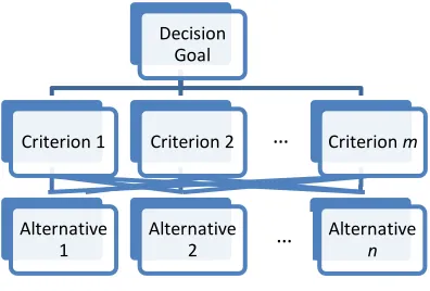
[image:12.612.204.402.72.206.2]

Figure 2: AHP hierarchical structure

The AHP provides a comprehensive and rational framework for representing and quantifying the elements of decision problems, relating those elements to overall goals, and evaluating alternative solutions. Applying the AHP to a decision problem involves four steps: 1) structuring the problem into a hierarchical model, 2) comparing elements of the problem to one another to generate pairwise comparison matrices, 3) calculating the weight or priority of each element in the hierarchy, and 4) aggregating the weights across various levels to obtain the final weights of the alternatives. (See [8].)

Pairwise comparison matrices are an integral part of the AHP, indicating how much more important one objective might be than another. Let

A = = [

] (1)

be a pairwise comparison matrix for a single decision maker. The entry in row i and column j of A indicates how much more important objective i is than objective j, with = 1 for all i and =

1/ for j ≠ i. How to calculate priorities from a pairwise comparison matrix has been the focus

of several studies, with techniques aimed at deriving a priority vector including: the eigenvector method [9], the weighted least-square method (WLSM) [10], the logarithmic least square method (LLSM) [11], and the fuzzy programming method [12].

Decision Goal Criterion 1 Alternative 1 Criterion 2 Alternative 2

Criterion m

Alternative

n …

(13)

10

3.3 DEAHP

In 2006, Ramanathan [13] developed a method that uses data envelopment analysis (DEA) for generating local weights of alternatives from pairwise comparison matrices in the AHP. DEA is a linear programming based approach used to determine the productive efficiency of a system or decision-making-unit (DMU) (e.g., a university, hospital, or restaurant) by comparing how well the DMU converts inputs into outputs. The DMU that produces the largest amount of outputs by consuming the least amount of inputs is considered to have an efficiency score of one. The efficiencies of the other DMUs are obtained relative to the efficient DMU, and are assigned efficiency scores between zero and one [8]. Ramanathan’s method, referred to as DEAHP, considers each criterion or alternative in a pairwise comparison matrix as a DMU. The row elements of the pairwise comparison matrix are viewed as the outputs of the DMUs, and a dummy input with a value of one is used to build a model that calculates the efficiency score for each DMU. The efficiency scores are then used as the local priorities of the DMUs, whether they are decision criteria or alternatives.

The DEAHP method succeeds in producing true weights for perfectly consistent pairwise comparison matrices, but was criticized by Wang et al [14] for not being able to produce rational weights for inconsistent pairwise comparison matrices. In addition, Wang et al [14] proved that the DEAHP may also produce illogical results for pairwise comparison matrices with satisfactory consistency. As a result, Wang and Chin [15] introduced a new DEA methodology in 2009.

3.4 DEA Methodology for Priority Determination in the Group AHP

(14)

11

from a group of pairwise comparison matrices, regardless of whether they are perfectly consistent or inconsistent.

Let

= = [

] (2)

be a pairwise comparison matrix provided by the kth decision maker (DMk) (k = 1,…, m),

where is the kth decision maker’s assessment of how important objective i is relative to

objective j, and m is the number of decision makers. In addition, let hk > 0 be the decision

maker’s relative importance weight satisfying ∑ , and ,…, be the decision variables. The following model is solved for each wi (i = 1,…,n) to obtain the best relative local

priorities of the n criteria or alternatives under group decision making. Subscript zero represents the decision criterion or alternative under evaluation, namely DMU0:

Maximize = ∑ ∑ (3)

Subject to{

∑ ∑∑ ∑ ∑

After the best local priorities for both criteria and alternatives have been derived by the DEA methodology, the final weight of each decision alternative can be computed using the simple additive weighting (SAW) method [9]. Let , …, be the best local priorities of the m decision criteria and , …, be the best local priorities of the n decision alternatives with

(15)

12

Final weight of Alternative = ∑ (4)

The above methodology is effective in assessing the value of different alternatives, given the assignment of the decision maker weights is correct. Decision maker weights are a)

determined by an outside decision maker, or b) agreed upon by the decision makers involved in the decision making process. For certain group decision making problems, though, there might not be any individuals outside of the problem who are qualified to assign decision maker weights, or if a group decision making problem is highly classified, having an outside decision maker assign decision maker weights is not an option. When decision makers must work together to identify their weights, they must discuss their qualifications for making the decision with each other. This can be an impractical and even inconvenient conversation to have,

especially when members of the group have to identify who among them is least qualified to address the problem. A method for calculating decision maker weights using the members of the group in an anonymous manner is essential to preserving the integrity of the group decision making process.

We propose to adapt the DEA methodology proposed by Wang and Chin [15] to address the vaccine prioritization problem. To do this, we will expand Wang and Chin’s model for group decision making to calculate not only the local priorities of the criteria and alternatives, but also the weights of the decision makers, whose inputs will be used to provide feedback about stakeholder preferences and priorities. The following section reviews the proposed methodology.

3.5 Comprehensive DEA Methodology for Priority Determination in the Group AHP

(16)

13

Let

= = [

] (5)

be a pairwise comparison matrix provided by the kth decision maker ) (k = 1,…, d), where

_{is the kth decision maker’s assessment of how qualified decision maker}_i_{is relative to}

decision maker j for assessing the given problem. The linear programming model in (6) is solved for each (i = 1,…,d) to obtain the weights of the d decision makers involved in group decision making:

Subject to{

∑ ∑∑ ∑ ∑

For the model (6), is the relative weight or score for decision maker i and is the score of decision maker j with respect to decision maker i. In addition, h is the initial weight of each decision maker and is equal to 1/d. The first constraint requires the sum of the output values with respect to each decision maker to equal one. The second constraint is a product of Saaty’s eigenvector method [9].

Next, let

= = [

] (7)

(17)

14

goal. The linear programming model in (8) is solved for each CRi (i = 1,…,c) to obtain the

weights of the c criteria related to the given problem:

Subject to{

∑ ∑∑ ∑ ∑

For the model (8), is the relative weight or score for criterion i and is the score of criterion j with respect to criterion i. In addition, is the weight of each decision maker as calculated by model (6). The first constraint requires the sum of the output values with respect to each criterion to equal one. The second constraint is a product of Saaty’s eigenvector method [9].

Now, let

= = [

] (9)

be a pairwise comparison matrix provided by the kth decision maker where is the kth decision maker’s assessment of how project i compares to project j with respect to criteria l. The linear programming model in (10) is solved for each PCRil (i = 1,…,p. l = 1,…,c.) to obtain the

weight of each project with respect to the each criteria:

Maximize = ∑ ∑ , (10)

Subject to{

∑ ∑ ∑

∑ ∑

(18)

15

For the model (10), is the relative weight or score for project i with respect to

criterion l and is the score of project j with respect to criterion l with respect to the

project-criterion being evaluated (project i with respect to criterion l). In addition, is the weight of each decision maker as calculated by model (6). The first constraint requires the sum of the output values with respect to each project-criterion to equal one. The second constraint is a product of Saaty’s eigenvector method [9].

Lastly, the final weight of each initiative can be computed using the simple additive weighting (SAW) method [9]. Let , …, be the best local priorities of the c decision criteria and , …, be the best local priorities of the i decision alternatives with respect

to the lth criterion (l = 1,…, c). Equation (4) can be used to calculate the final weight of each decision alternative.

Final weight of Alternative = ∑ (11)

3.6 Arrow’s Impossibility Theorem

According to Arrow’s impossibility theorem [16], when voters have three or more distinct alternatives, no rank order voting system can convert the ranked preferences of individuals into a community-wide ranking while also meeting the following criteria:

- If every voter prefers alternative A to alternative B, then the group prefers A to B.

(19)

16

- There are no dictators; no single voter possesses the power to always determine the group’s preference.

The Comprehensive DEA Methodology for Priority Determination in the Group AHP (CDEAGAHP) is a rank-order system that was designed to satisfy the first two criteria while allowing decision makers to have different weights of influence over the decision-making process. If every voter prefers alternative A to alternative B, then the group ranking will have alternative A ranked above alternative B. If an alternative is eliminated from consideration, then the new ordering for the remaining alternatives will be equivalent to the original ordering minus the eliminated alternative (IIA). Lastly, the CDEAGAHP allows a decision maker to have more weight than other decision makers by applying the AHP and DEA to derive weights based on peer evaluations.

An illustrative example that demonstrates an application of the Comprehensive DEA Methodology for Priority Determination in the Group AHP (CDEAGAHP) is explained in Appendix A. The following section applies the methodology to a vaccine prioritization problem.

4. Vaccine Prioritization Using the Comprehensive DEA Methodology for

Priority Determination in the Group AHP

Data was gathered to apply the Comprehensive DEA Methodology for Priority

(20)

17

represent the interests of the private sector, and one was chosen to represent the interests of non-governmental organizations. These decision makers are listed in Table 10.

Table 10: Vaccine Example Decision Makers

Decision Maker Sector

Health Agency Representative Pubic Public Health Unit Representative Public Vaccine Industry Representative Private Biopharmaceutical Industry Representative Private

International Vaccine Initiative Representative Non-governmental Organization

Ten criteria were chosen for the experiment that are similar to some of the 29 criteria used in the 2012 IOM model. Criteria were chosen to capture the health, economic,

demographic, scientific, business, and programmatic considerations associated with vaccine development. The ten criteria are listed in Table 11.

Table 11: Vaccine Example Criteria

Criterion Definition

Target Population Vaccine targets a disease that affects a population of interest

Cost-Effectiveness $/QALY gained

Incident Cases Prevented Per Year Through Vaccination

The number of incident cases of disease prevented in one year

(21)

18

Potential to Improve Delivery Methods Vaccine development has the potential to improve delivery methods or stimulate novel

approaches to deliver vaccines Premature Deaths Averted Per Year Through

Vaccination

The number of deaths due to disease prevented in one year

QALYs Gained Net increase in QALYs gained in the population vaccinated

Reduces Challenges Relating to Cold Chain Requirements

Vaccine development has the potential to stimulate novel approaches to mitigate the challenges relating to cold-chain storage and

related packaging. Healthcare Cost Reduction Health care costs saved

Time to Licensure The estimated length of time until successful licensure

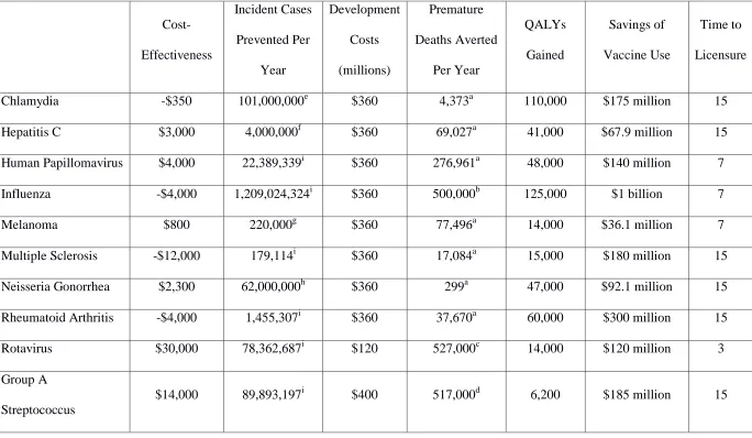
For the vaccine candidates, ten were chosen as a subset of the 26 vaccine candidates that were used for evaluation in “Vaccines for the 21st Century” [6]. The ten vaccine candidates are: ‘Chlamydia’, ‘Group A Streptococcus’, ‘Hepatitis C’, ‘Human Papillomavirus’, ‘Influenza’, ‘Melanoma’, ‘Multiple Sclerosis’, ‘Neisseria Gonorrhea’, ‘Rheumatoid Arthritis’, and ‘Rotavirus’.

(22)

19

him or herself, in order of ability to prioritize vaccine candidates. For the ranking, the first position would be for the decision maker with the most ability to prioritize vaccine candidates, while the last position would be for the decision maker with the least ability to prioritize vaccine candidates. If someone thought that two or more decision makers were equal in rank, they could rank them in the same position. Before these rankings would occur, though, each decision maker would have the opportunity to review the CV’s of the other decision makers to gain an

understanding of their experience with vaccine development.

After ranking the decision makers, each decision maker would then rank the criteria of evaluation in order of importance for prioritizing vaccine candidates. For the ranking, the first position would be for the criterion that the decision maker thinks is most important to consider when prioritizing vaccine candidates, while the last position would be for the criterion that the decision maker thinks is least important to consider when prioritizing vaccine candidates. If a decision maker considered two or more criteria to be equal in performance, they could rank them in the same position.

(23)

20

Given that this is a derived experiment, assumptions were made about how the decision makers might assess each other, the criteria, and the vaccine candidates with respect to the qualitative criteria. The rankings that were created for each decision maker were used to generate the pairwise comparison matrices for the model. The pairwise comparison matrices were created according to the following rules: 1) is an integer valued 1-10, 2) = 1/ , 3) = 1 for all i,

3) if the rank of option i, ( ), and the rank of option j, ( ), are equal, then elements and

equal one, 4) if > , then aij equals ( – + 1).

Typically, decision makers would create pairwise comparison matrices themselves rather than record rankings of the decision makers, criteria, and alternatives, but constructing pairwise comparison matrices is a cumbersome task for decision makers when more than a few criteria are considered. In the case where actual decision makers would be using this model, it was decided that it would be easier for decision makers to rank their preferences so pairwise comparison matrices could be generated from those rankings.

(24)

[image:24.792.71.755.97.495.2]

21

Table 12: Vaccine Example Quantitative Data

Cost-Effectiveness

Incident Cases Prevented Per

Year

Development Costs (millions)

Premature Deaths Averted

Per Year

QALYs Gained

Savings of Vaccine Use

Time to Licensure

Chlamydia -$350 101,000,000e $360 4,373a 110,000 $175 million 15 Hepatitis C $3,000 4,000,000f $360 69,027a 41,000 $67.9 million 15 Human Papillomavirus $4,000 22,389,339i $360 276,961a 48,000 $140 million 7 Influenza -$4,000 1,209,024,324i $360 500,000b 125,000 $1 billion 7

Melanoma $800 220,000g $360 77,496a 14,000 $36.1 million 7

Multiple Sclerosis -$12,000 179,114i $360 17,084a 15,000 $180 million 15 Neisseria Gonorrhea $2,300 62,000,000h $360 299a 47,000 $92.1 million 15 Rheumatoid Arthritis -$4,000 1,455,307i $360 37,670a 60,000 $300 million 15 Rotavirus $30,000 78,362,687i $120 527,000c 14,000 $120 million 3 Group A

Streptococcus

(25)

22

Note. Data for ‘Cost-Effectiveness’, ‘Development Costs’, ‘QALYs Gained’, ‘Savings of Vaccine Use’, and ‘Time to Licensure’ from “Vaccines for the 21st

Century” [6].

a. "Global Health Observatory Data Repository." Cause-specific Mortality, 2008: WHO Region by Country. N.p., n.d. Web. <http://apps.who.int/gho/data/node.main.887?lang=en>.

b. "Influenza (Seasonal)." WHO. N.p., n.d. Web. <http://www.who.int/mediacentre/factsheets/fs211/en/>.

c. Parashar, Umesh D., et al. "Global mortality associated with rotavirus disease among children in 2004." Journal of Infectious Diseases 200.Supplement 1 (2009): S9-S15.

d. Carapetis, Jonathan R. "The current evidence for the burden of group A streptococcal diseases." Geneva: World Health Organization (2004): 1-57.

e. "Prevalence and Incidence of Selected Sexually Transmitted Infections." WHO. N.p., n.d. Web. <http://whqlibdoc.who.int/publications/2011/9789241502450_eng.pdf>.

f. "Hepatitis C." WHO. N.p., n.d. Web. <http://www.who.int/mediacentre/factsheets/fs164/en/>.

g. "Global Health Observatory Data Repository." Incidence: WHO Region by Country. N.p., n.d. Web. <http://apps.who.int/gho/data/node.main.903?lang=en>.

h. "Sexually Transmitted Diseases." WHO. N.p., n.d. Web. <http://www.who.int/vaccine_research/diseases/soa_std/en/index2.html>.

(26)

23

[image:26.612.126.484.159.374.2]

Table 13 shows the weight assigned to each decision maker as determined by the linear programming model in (6).

Table 13: Vaccine Example Decision Maker Weights

Decision Maker Weight

Public Health Unit Representative

0.247393

Health Agency Representative 0.217927 Vaccine Industry Representative 0.1999291

International Vaccine Initiative Representative

0.19927

Biopharmaceutical Industry Representative

0.190454

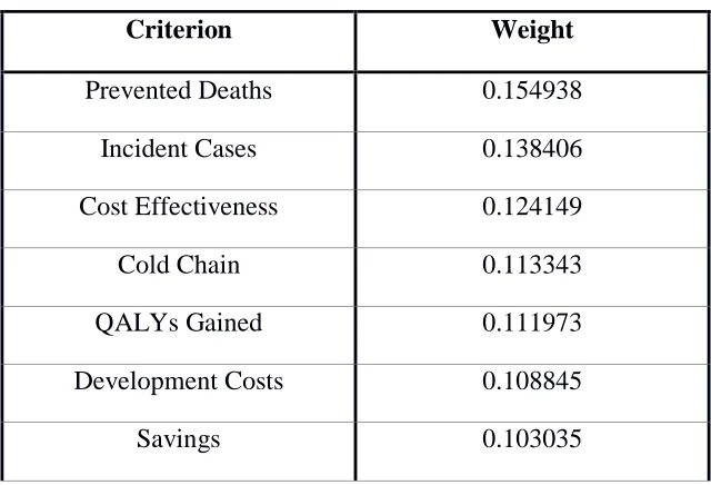
[image:26.612.128.482.162.373.2]

Table 14 shows the weight assigned to each criterion as determined by the linear programming model in (8).

Table 14: Vaccine Example Criterion Weights

Criterion Weight

Prevented Deaths 0.154938 Incident Cases 0.138406 Cost Effectiveness 0.124149

Cold Chain 0.113343

QALYs Gained 0.111973

Development Costs 0.108845

[image:26.612.146.466.484.702.2]

(27)

24

Time to Licensure 0.0862401 Delivery Methods 0.0726194 Priority Population 0.0552014

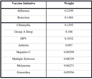
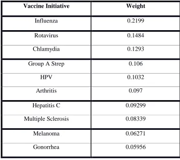
[image:27.612.129.482.279.576.2]

Table 15 shows the ranking of vaccine candidates produced by the linear programming model in (10).

Table 15: Model Vaccine Candidate Ranking

Vaccine Initiative Weight

Influenza 0.2199

Rotavirus 0.1484

Chlamydia 0.1293

Group A Strep 0.106

HPV 0.1032

Arthritis 0.097

Hepatitis C 0.09299

Multiple Sclerosis 0.08339

Melanoma 0.06271

Gonorrhea 0.05956

(28)

25

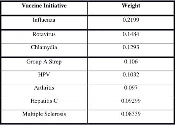
[image:28.612.128.482.216.521.2]

Lastly, the k-means clustering algorithm [17] was used to sort the vaccine candidates into clusters and identify which vaccine candidates are similar in overall performance with respect to the final ranking. Tables 16 through 19 show the clusters that result from applying the k-means algorithm with k = 2 to k = 5.

Table 16: Vaccine Example k-means Clustering: k=2

Influenza 0.2199

Rotavirus 0.1484

Chlamydia 0.1293

Group A Strep 0.106

HPV 0.1032

Arthritis 0.097

Hepatitis C 0.09299

Melanoma 0.06271

(29)

26

Influenza 0.2199

Rotavirus 0.1484

Chlamydia 0.1293

Group A Strep 0.106

HPV 0.1032

Arthritis 0.097

Hepatitis C 0.09299

Melanoma 0.06271

[image:29.612.130.482.450.702.2]

Gonorrhea 0.05956

Influenza 0.2199

Rotavirus 0.1484

Chlamydia 0.1293

Group A Strep 0.106

HPV 0.1032

Arthritis 0.097

Hepatitis C 0.09299

(30)

27

Melanoma 0.06271

[image:30.612.128.480.180.493.2]

Gonorrhea 0.05956

Table 19: Vaccine Example k-means clustering: k=5

Influenza 0.2199

Rotavirus 0.1484

Chlamydia 0.1293

Group A Strep 0.106

HPV 0.1032

Arthritis 0.097

Hepatitis C 0.09299

Melanoma 0.06271

Gonorrhea 0.05956

(31)

28

‘Rotavirus’, but there is a significant difference between the rankings of these two vaccine candidates and ‘Influenza’.

5. Sensitivity Analysis

The goal of sensitivity analysis is to understand how changes in a problem’s parameters affect the problem’s solution. In the case of the vaccine prioritization problem, it is important to understand how changes in the decision maker’s preferences might affect the final ranking of alternatives. Consider the objective function of model (6):

= ∑ ∑

For this problem, it is important to know how a decision maker’s assessment of his/her fellow decision makers can change without affecting the final ranking of alternatives. Using sensitivity analysis, the objective function coefficient ranges were determined; within these ranges, the current basis remains optimal. For this problem, that provides the range of∑ for each . This range must be divided by h to determine how the summation of the decision makers’ assessments (∑ ) can vary when comparing decision maker to decision maker .

(32)

29

Table 12: Objective Function Coefficient Ranges

Decision Makers

j = Health Agency j = Public Health j= Vaccine Industry

∑ Lower Bound ∑ Upper Bound ∑ Lower Bound ∑ Upper Bound ∑ Lower Bound ∑ Upper Bound

i = Health Agency 4.8725 5.78 -5.00E+100 4.624 6.675 21.195

i = Public Health 5.415 6.685 -5.00E+100 5.57 7.925 32.235

i = Vaccine Industry 4.631 31.815 4.347 35.01 -5.00E+100 5.77

i = BiopharmIndustry 3.6505 44.575 3.4355 52.25 4.4285 5.00E+100

i = InternationalVacInit 4.427 5.19 4.6505 26.7 6.605 24.77

Table 12: Objective Function Coefficient Ranges (cont.)

Decision Makers

j = BiopharmIndustry j = InternationalVacInit

∑ Lower Bound ∑ Upper Bound ∑ Lower Bound ∑ Upper Bound

i = Health Agency 7.415 21.555 5.67 23.9

i = Public Health 8.845 29.855 6.77 87.4

i = Vaccine Industry 5.64 8.19 5.11 45.865

i = BiopharmIndustry -5.00E+100 5.64 3.993 68.65

i = InternationalVacInit 7.365 21.33 -5.00E+100 5.625

(33)

30

coefficient can vary within the range shown in Table 12 and not affect the value of or the final ranking of alternatives. The ranges highlighted in Table 12 are associated with nonbasic

variables. For these ranges, the summation of the decision makers’ preferences can vary within this range and not change the value of or the final ranking of alternatives.

To understand how the final ranking of alternatives might also be affected by the weight of the decision makers, sensitivity analysis was performed to determine how a single decision maker’s weight can vary such that the ranking of a single vaccine candidate will remain the same. As an example, the weight of ‘Health Agency Representative’ was analyzed to see how it can vary such that the ranking of ‘Chlamydia’ will remain the same. A vaccine candidate’s ranking will remain the same if the weight associated with it is greater than the weight of the vaccine candidate ranked below it and less than the weight of the vaccine candidate ranked above it. In this case, the weight of ‘Chlamydia’ must be greater than or equal to 0.1061 and less than or equal to 0.1483 to remain the same.

To determine the range for which the weight of ‘Health Agency Representative’ can vary such that the ranking of ‘Chlamydia’ will remain the same, equations 12 and 13 were solved.

∑ ≤ (12)

∑ ≥ (13)

The functions for each criterion ( ) and for ‘Chlamydia’ with respect to each criterion ( ) were rewritten in terms of the values associated with those functions and

. Each equation was solvedfor which represents the value that can be

(34)

31

can be found in Appendix K. The results of the analysis suggest that the weight of ‘Health Agency Representative’ can vary between 0 and 0.321654 without affecting the final ranking of ‘Chlamydia’. A large range would suggest that ‘Health Agency Representative’ has little to no influence over the ranking of ‘Chlamydia’, while a small range would suggest that ‘Health Agency Representative’ has a significant influence over the ranking of ‘Chlamydia’. In this case, ‘Health Agency Representative’ has a small influence over the ranking of ‘Chlamydia’.

6. Conclusions

The Comprehensive DEA Methodology for Priority Determination in the Group AHP (CDEAGAHP) does an effective job of calculating decision maker weights, criterion weights, and weights for each project with respect to each criterion to come up with a final weight for each project. The CDEAGAHP provides a methodology for calculating decision maker weights using the members of the group in an anonymous manner which is essential to preserving the integrity of the group decision making process. The methodology can be applied to any multiple criteria decision making (MCDM) problem that involves multiple decision makers evaluating multiple alternatives and assessing them according to a variety of quantitative and qualitative criteria. Examples of MCDM problems the methodology can be applied to include choosing a new vehicle for a company to purchase or identifying which vaccine candidates should receive

increased attention and funding around the world. The rankings generated by the model are

frequently consistent with the data related to the projects and the rankings provided by the

(35)

32

Future work related to this problem includes evaluating alternative methods for incorporating quantitative data into the model. Presently, quantitative data is gathered about each project with respect to a particular criterion and the projects are ranked according to how they perform with respect to that criterion. That ranking is then used to generate the pairwise comparison matrix for all of the decision makers. Alternative methods could be used to incorporate this data.

(36)

33

References.

[1] U.S. Department of Health and Human Services. 2011. 2010 National Vaccine Plan. Washington, DC: U.S. Department of Health and Human Services.

[2] Institute of Medicine. 2012. Ranking Vaccines: A Prioritization Framework: Phase I:

Demonstration of Concept and a Software Blueprint. Washington, DC: National Academy Press. [3] World Health Organization. 2000. Assessing the global needs for vaccine research and development. Geneva, Switzerland.

[4] Institute of Medicine. 1985. New Vaccine Development: Establishing Priorities, Volume I. Diseases of Importance in the United States. Washington, DC: National Academy Press. [5] Institute of Medicine. 1986. New Vaccine Development: Establishing Priorities, Volume II. Diseases of Importance in Developing Countries. Washington, DC: National Academy Press. [6] Institute of Medicine. 2000. Vaccines for the 21st Century: A Tool for Decisionmaking. Washington, DC: National Academy Press.

[7] Saaty, Thomas L. The Analytic Hierarchy Process: Planning, Priority Setting, Resource Allocation. New York: McGraw-Hill, 1980.

[8] Winston, Wayne L. Operations Research: Applications and Algorithms. 4th ed. Belmont: Brooks/Cole, 2004.

[9] Saaty, Thomas L. Fundamentals of decision making and priority theory with the analytic hierarchy process. RWS Publications, 1994.

[10] Chu, A. T. W., R. E. Kalaba, and K. Spingarn. "A comparison of two methods for determining the weights of belonging to fuzzy sets." Journal of Optimization Theory and Applications 27.4 (1979): 531-538.

[11] Crawford, G. B. "The geometric mean procedure for estimating the scale of a judgement matrix." Mathematical Modelling 9.3 (1987): 327-334.

[12] Mikhailov, Ludmil. "A fuzzy programming method for deriving priorities in the analytic hierarchy process." Journal of the Operational Research Society 51.3 (2000): 341-349. [13] Ramanathan, Ramakrishnan. "Data envelopment analysis for weight derivation and

aggregation in the analytic hierarchy process." Computers & Operations Research 33.5 (2006): 1289-1307.

[14] Wang, Ying-Ming, Celik Parkan, and Ying Luo. "A linear programming method for generating the most favorable weights from a pairwise comparison matrix."Computers & Operations Research 35.12 (2008): 3918-3930.

[15] Wang, Ying-Ming, and Kwai-Sang Chin. "A new data envelopment analysis method for priority determination and group decision making in the analytic hierarchy process." European Journal of Operational Research 195.1 (2009): 239-250.

[16] Arrow, Kenneth J. "A difficulty in the concept of social welfare." The Journal of Political Economy 58.4 (1950): 328-346.

(37)

34 Appendix A: Vehicle Experiment

The purpose of this experiment was to ensure that the DEA methodology for priority determination in the group AHP can be extended to include the determination of decision maker weights. This experiment serves as an illustrative example of the proposed methodology and demonstrates how the methodology can be applied to other problems with multiple criteria and decision makers. The methodology explained in Section 3.4 is used to calculate the weights of the decision makers, criteria, and alternatives.

(38)

35

Table 1: Vehicle Characteristics

2009 Ford F150 XLT 2013 Chrysler Town & Country Limited 2012 Jeep Grand Cherokee Laredo 2012 Toyota Camry SE 2002 Nissan Altima 2.5 S

2006 Dodge Grand Caravan SE 2012 Chevrolet Silverado 1500 LT 2006 Honda CR-V SE

Price $17,994 $38,646 $25,991 $22,700 $5,995 $7,988 $27,869 $13,995

Mileage 49,832 mi.

12 mi. 29,288 mi.

7,658 mi. 97,176 mi.

60,500 mi.

7,225 mi. 85,000 mi.

Gas Mileage

14-15 mpg (city) / 18

-20 mpg (highway)

17 mpg (city) / 25

mpg (highway) 12-17 mpg (city) / 18-23 mpg (highway) 21-25 mpg (city) / 30-35 mpg (highway) 19-23 mpg (city) / 26-29 mpg (highway) 19-20 mpg (city) / 26

mpg (highway) 12-15 mpg (city) / 18-22 mpg (highway) 21-23 mpg (city) /

26-29 mpg (highway)

Body Style

Pickup Minivan SUV Sedan Sedan Minivan Pickup SUV

(39)

[image:39.612.137.477.87.293.2]

36

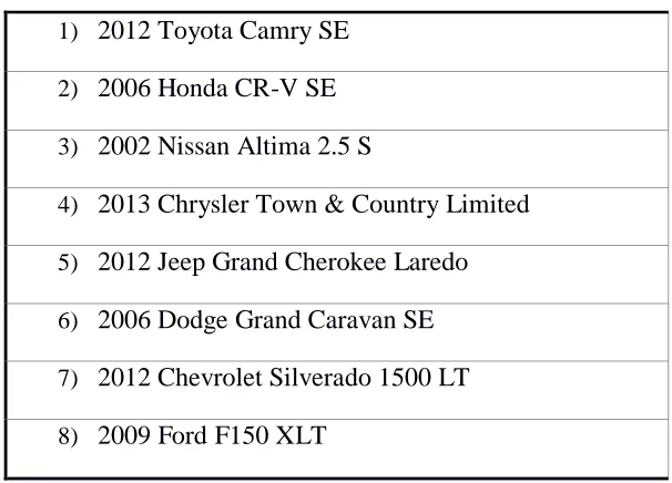
Table 2: Group 1 Vehicle Ranking

1) 2012 Toyota Camry SE

2) 2012 Jeep Grand Cherokee Laredo

3) 2006 Honda CR-V SE

4) 2002 Nissan Altima 2.5 S

5) 2006 Dodge Grand Caravan SE

6) 2013 Chrysler Town & Country Limited

7) 2012 Chevrolet Silverado 1500 LT, 2009 Ford F150 XLT

Following this activity, each member of the group was asked to independently fill out a packet that had them rank the decision makers, criteria of evaluation, and vehicles in comparison to the criteria. These rankings were requested to provide the information necessary to generate the pairwise comparison matrices for the model.

(40)

37

After ranking the decision makers, each person had to rank the criteria of evaluation in order of importance in choosing a vehicle for the company to purchase. The criteria of evaluation were: gas mileage, color, cost, body style, make, appearance, features, and mileage. For the ranking, the first position was for the criterion that was most important to consider when choosing a vehicle for the company to purchase, while the eighth position was for the criterion that was least important to consider when choosing a vehicle for the company to purchase. If two or more criteria were considered equal in importance, a decision maker could rank them in the same position.

Lastly, the decision makers were asked to rank the vehicles in order of preference for the qualitative criteria (color, body style, make, appearance, and features). For these rankings, the first position was for the vehicle that the decision maker thought best satisfied that criterion, while the eighth position was for the vehicle that the decision maker thought least satisfied that criterion. If two or more vehicles were considered equal in satisfying a certain criterion, a decision maker could rank them in the same position.

(41)

38

valued 1-9, 2) = 1/ , 3) = 1 for all i, 3) if the rank of option i, , and the rank of option j,

, were equal, then element and equaled one, 4) if > , then aij equaled ( – + 1).

[image:41.612.130.480.377.647.2]

For the quantitative criteria ‘cost’ and ‘mileage’, the vehicles were ranked in ascending order, and for the quantitative criteria ‘gas mileage’, the vehicles were ranked in descending order. The resulting rankings were then used to generate the appropriate pairwise comparison matrices using the method described above.

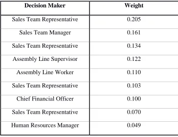
Table 3 shows the weight assigned to each decision maker for Group 1, as determined by the model and the rankings provided by all of the decision makers. The weights assigned to each decision maker for the rest of the groups can be found in Appendix C.

Table 3: Group 1 Decision Maker Weights

Sales Team Representative 0.205

Sales Team Manager 0.161

Sales Team Representative 0.134 Assembly Line Supervisor 0.122

Assembly Line Worker 0.110

Sales Team Representative 0.103 Chief Financial Officer 0.100 Sales Team Representative 0.070 Human Resources Manager 0.049

When the decision makers were ranking the decision makers in the group, they were

(42)

39

vehicles. This is evident by the resulting decision maker weights. In most cases, the individuals

with the most weight were a) part of the sales team, the group that would be using the new

vehicle, or b) the ones who seemed to have the most experience with vehicles based on the group

discussions. The individuals with the least weight seemed to have a lesser knowledge of vehicles

based on the group discussions, causing their peers to rank them low on their individual

assessments, regardless of their position in the company. This in turn resulted in them receiving

the least amount of influence in determining which vehicle the company should purchase.

Table 4 shows the weight assigned to each criterion for Group 1, as determined by the rankings provided by all of the decision makers. The weights assigned to each criterion for the rest of the groups can be found in Appendix D.

Table 4: Group 1 Criterion Weights

Gas Mileage 0.235

Cost 0.185

Mileage 0.173

Body Style 0.158

Make 0.112

Features 0.106

Appearance 0.075

(43)

40

For most of the groups, ‘gas mileage’, ‘cost’, and ‘mileage’ were given higher consideration to than the other criteria, while ‘color’, ‘features’, and ‘make’ were given less consideration to than the other criteria.

[image:43.612.154.457.251.469.2]

Table 5 shows the ranking of vehicles produced by the model for Group 1. The ranking of vehicles produced by the model for the rest of the groups can be found in Appendix E.

Table 5: Group 1 Model Vehicle Ranking

1) 2012 Toyota Camry SE

4) 2013 Chrysler Town & Country Limited

5) 2012 Jeep Grand Cherokee Laredo

7) 2012 Chevrolet Silverado 1500 LT

8) 2009 Ford F150 XLT

(44)

41

frequently moved up in rank between the group and model rankings. In these instances, the model was simply accounting for the criteria that the decision makers determined to be significant.

Lastly, the k-means clustering algorithm [16] was used to sort the vehicles into clusters and identify which vehicles were similar in overall performance according to the final ranking. Tables 6 through 9 show the clusters that result from applying the k-means algorithm to Group 1’s results with k = 2 to k = 5. The results of k-means clustering for the other groups can be found in Appendices F-J.

Table 6: Group 1 K-means clustering: k = 2 1) 2012 Toyota Camry SE

2) 2006 Honda CR-V SE 3) 2002 Nissan Altima 2.5 S

4) 2013 Chrysler Town & Country Limited 5) 2012 Jeep Grand Cherokee Laredo 6) 2006 Dodge Grand Caravan SE 7) 2012 Chevrolet Silverado 1500 LT 8) 2009 Ford F150 XLT

(45)

42

(46)

43 Appendix B: Vehicle Example Group Vehicle Rankings

Table B1: Group 2 Vehicle Ranking 1) 2012 Toyota Camry SE

2) 2012 Jeep Grand Cherokee Laredo 3) 2013 Chrysler Town & Country Limited

4) 2006 Honda CR-V SE, 2006 Dodge Grand Caravan SE 5) 2012 Chevrolet Silverado 1500 LT

6) 2002 Nissan Altima 2.5 S 7) 2009 Ford F150 XLT

4) 2013 Chrysler Town & Country Limited 5) 2012 Jeep Grand Cherokee Laredo 6) 2002 Nissan Altima 2.5 S

7) 2012 Chevrolet Silverado 1500 LT, 2009 Ford F150 XLT

2) 2012 Jeep Grand Cherokee Laredo 3) 2006 Honda CR-V SE

(47)

44

6) 2013 Chrysler Town & Country Limited 7) 2009 Ford F150 XLT

8) 2012 Chevrolet Silverado 1500 LT

2) 2012 Jeep Grand Cherokee Laredo 3) 2006 Honda CR-V SE

4) 2006 Dodge Grand Caravan SE 5) 2002 Nissan Altima 2.5 S

6) 2013 Chrysler Town & Country Limited 7) 2012 Chevrolet Silverado 1500 LT 8) 2009 Ford F150 XLT

2) 2012 Jeep Grand Cherokee Laredo 3) 2013 Chrysler Town & Country Limited 4) 2006 Honda CR-V SE

5) 2002 Nissan Altima 2.5 S 6) 2006 Dodge Grand Caravan SE

(48)

[image:48.612.142.468.124.392.2]

45 Appendix C: Vehicle Example Decision Maker Weights

Table C1: Group 2 Decision Maker Weights

Sales Team Representative 0.203857 Assembly Line Supervisor 0.178611 Sales Team Representative 0.147251 Sales Team Representative 0.139284 Human Resources Manager 0.137797 Sales Team Manager 0.105846 Sales Team Representative 0.0490293

Assembly Line Worker 0.0430622 Chief Financial Officer 0.0348999

[image:48.612.143.469.440.684.2]

(49)

[image:49.612.132.470.97.364.2]

46

[image:49.612.142.469.412.656.2]

Sales Team Manager 0.166367 Chief Financial Officer 0.164945 Human Resources Manager 0.160456 Sales Team Representative 0.13028 Sales Team Representative 0.12123 Sales Team Representative 0.118721 Sales Team Representative 0.113491 Assembly Line Supervisor 0.113004 Assembly Line Worker 0.0497484

Sales Team Manager 0.288403 Chief Financial Officer 0.192078 Human Resources Manager 0.150424 Sales Team Representative 0.134789 Sales Team Representative 0.121699 Sales Team Representative 0.107403 Assembly Line Supervisor 0.0461601

(50)

47

(51)

[image:51.612.145.467.124.366.2]

48 Appendix D: Vehicle Example Criterion Weights

Table D1: Group 2 Criterion Weights

Mileage 0.211369

Cost 0.206324

Appearance 0.16657

Gas Mileage 0.153486

Body Style 0.114927

Make 0.0996222

Features 0.0741825

Color 0.0687389

Cost 0.211628

Mileage 0.181939

Appearance 0.125923

Body Style 0.125665

Make 0.0947138

Features 0.0880294

[image:51.612.149.466.413.657.2]

(52)

[image:52.612.147.466.95.337.2]

49

Appearance 0.225753

Cost 0.214722

Mileage 0.176551

Body Style 0.157368

Features 0.0885038

Make 0.0627282

[image:52.612.149.466.399.642.2]

Color 0.0287769

Mileage 0.205662

Cost 0.203233

Appearance 0.154181

Body Style 0.0982986

Features 0.0919879

Make 0.057545

(53)

[image:53.612.149.466.95.339.2]

50

Body Style 0.261357

Mileage 0.202141

Appearance 0.173748

Cost 0.102853

Make 0.0711132

Color 0.0506744

(54)

[image:54.612.145.467.124.367.2]

51 Appendix E: Vehicle Example Model Vehicle Ranking

Table E1: Group 2 Model Vehicle Ranking

Vehicle Weight

1) Toyota 0.21226

2) Jeep 0.162489

3) Nissan 0.1478

4) Chrysler 0.145391

5) Honda 0.137473

6) Chevy 0.125838

7) Dodge 0.116254

8) Ford 0.0961831

1) Toyota 0.234231

2) Nissan 0.167109

3) Honda 0.159574

5) Dodge 0.138073

6) Jeep 0.117067

7) Chevy 0.102084

[image:54.612.149.466.415.659.2]

(55)

[image:55.612.148.467.95.338.2]

52

1) Toyota 0.233732

2) Nissan 0.176567

3) Jeep 0.16396

5) Honda 0.157053

6) Chevy 0.120783

7) Dodge 0.117781

8) Ford 0.0891504

1) Toyota 0.241221

2) Nissan 0.161906

3) Honda 0.149379

5) Jeep 0.126731

6) Dodge 0.114109

7) Chevy 0.110166

[image:55.612.150.466.386.630.2]

(56)

[image:56.612.149.466.95.339.2]

53

1) Toyota 0.220474

2) Nissan 0.152795

3) Jeep 0.148616

5) Honda 0.136383

6) Chevy 0.135783

7) Dodge 0.0940066

(57)

54 Appendix F: Vehicle Example Group 2 k-means Clustering

Table F1: Group 2 K-means clustering: k = 2 1) 2012 Toyota Camry SE

2) 2012 Jeep Grand Cherokee Laredo 3) 2002 Nissan Altima 2.5 S

4) 2013 Chrysler Town & Country Limited 5) 2006 Honda CR-V SE

6) 2012 Chevrolet Silverado 1500 LT 7) 2006 Dodge Grand Caravan SE 8) 2009 Ford F150 XLT

(58)

[image:58.612.155.461.93.230.2]

55

(59)

56 Appendix G: Vehicle Example Group 3 k-means Clustering

Table G1: Group 3 K-means clustering: k = 2 1) 2012 Toyota Camry SE

2) 2002 Nissan Altima 2.5 S 3) 2006 Honda CR-V SE

4) 2013 Chrysler Town & Country Limited 5) 2006 Dodge Grand Caravan SE

6) 2012 Jeep Grand Cherokee Laredo 7) 2012 Chevrolet Silverado 1500 LT 8) 2009 Ford F150 XLT

(60)

[image:60.612.155.460.93.230.2]

57

(61)

58 Appendix H: Vehicle Example Group 4 k-means Clustering

Table H1: Group 4 K-means clustering: k = 2 1) 2012 Toyota Camry SE

(62)

[image:62.612.155.459.93.230.2]

59

(63)

60 Appendix I: Vehicle Example Group 5 k-means Clustering

Table I1: Group 5 K-means clustering: k = 2 9) 2012 Toyota Camry SE

10)2002 Nissan Altima 2.5 S 11)2006 Honda CR-V SE

12)2013 Chrysler Town & Country Limited 13)2012 Jeep Grand Cherokee Laredo 14)2006 Dodge Grand Caravan SE 15)2012 Chevrolet Silverado 1500 LT 16)2009 Ford F150 XLT

(64)

[image:64.612.154.459.93.230.2]

61

(65)

62 Appendix J: Vehicle Example Group 6 k-means Clustering

Table J1: Group 6 K-means clustering: k = 2 17)2012 Toyota Camry SE

18)2002 Nissan Altima 2.5 S

19)2012 Jeep Grand Cherokee Laredo 20)2013 Chrysler Town & Country Limited 21)2006 Honda CR-V SE

22)2012 Chevrolet Silverado 1500 LT 23)2006 Dodge Grand Caravan SE 24)2009 Ford F150 XLT

Table J2: Group 6 K-means clustering: k = 3 1) 2012 Toyota Camry SE

(66)

63

(67)

64 Appendix K: Sensitivity Analysis Calculation

Final weight of Alternative = ∑ = 0.1293

0.1061 ≤ ≤ 0.1483

≥ ( ) +

( ) +

( ) + ( )

+ ( ) + ( ( ) +

( ) +

( + (

0.1483 ≥

(0.174248776 + (0.20745582))(0.094918693 + (0.08454348)) +

(0.100617054 + (0.120296914))(0.105894635 + (0.08376367)) +

(0.027392656 + (0.038151967))(0.052969646 + (0.09016668)) +

(0.17421749 + (0.20829227))(0.120315309 + (0.08301262)) +

(0.052596999 + (0.062884365))(0.076275375 + (0.04572506)) +

(0.075880705 + (0.0907221))(0.09001065 + (0.08642504)) +

(0.01607623 + (0.01922052))(0.136847309 + (0.08301262)) +

(0.052125907 + (0.054869718))(0.049243159 + (0.02734054)) +

(0.173912778 + (0.207928445))(0.093882309 + (0.08301262)) +

(68)

65 0.1483 ≥

0.0165394661 + (0.0147315979) + (0.0196914353) +

(0.017539037) 2 +

0.0106548062 + (0.0084280537) + (0.0127387978) +

(0.010076511) 2 +

0.0014509793 + (0.0024699048) + (0.0020208962) +

(0.0034400362) 2 +

0.0209610311 + (0.0144622503) + (0.0250607488) +

(0.0172908871 2 +

0.0040118558 + (0.0024050009) + (0.0047965285) +

(0.0028753914) 2 +

0.0068300716 + (0.006557993) + (0.0081659552) +

(0.0078406611) 2 +

0.0021999888 + (0.00133453) + (0.0026302764) +

(0.0015955457) 2 +

0.0025668443 + (0.0014251504) + (0.0027019582) +

(0.0015001677) 2 +

0.0163273332 + (0.0144369554) + (0.0195208025) +

(0.017260685) 2 +

0.0054109594 + (0.0056054798) + (0.0064692834) +

(0.0067018498) 2

0.1483 ≥ 0.0869533358 + (0.0718569162) + (0.1037966823) +

(0.086120772) 2

0.1483 ≥ 0.0869533358 + (0.1756535985) + (0.086120772) 2

(0.086120772) 2 + (0.1756535985) – 0.0613466642 ≤ 0

(69)

66 0.1061 ≤ 0.0869533358 + (0.1756535985) + (0.086120772) 2

(0.086120772) 2 + (0.1756535985) – 0.0191466642 ≥ 0

= -2.1433466462, 0.1037272324

= 0.217927

0.217927 – 2.34357 < xHA < 0.217927 + 0.103727