Exponential stability of the Euler-Maruyama method for neutral stochastic functional differential equations with jumps

.

.

SCIENCE CHINA

Information Sciences

Exponential stability of the Euler-Maruyama method

for neutral stochastic functional differential equations

with jumps

Haoyi MO

_{, Mengling LI}

_{, Feiqi DENG}

_{& Xuerong MAO}

1_{School of Applied Mathematics, Guangdong University of Technology, Guangzhou510006, China;} 2_{Systems Engineering Institute, South China University of Technology, Guangzhou510640, China;}

3_{Department of Mathematics and Statistics, University of Strathclyde, GlasgowG1 1XH, UK}

Received ; accepted

Abstract The exponential stability of trivial solution and the numerical solution for neutral stochastic func-tional differential equations (NSFDEs) with jumps is considered. The stability includes the almost sure expo-nential stability and the mean-square expoexpo-nential stability. New conditions for jumps are proposed by means of the Borel measurable function to ensure stability. It is shown that if the drift coefficient satisfies the linear growth condition, the Euler-Maruyama method can reproduce the corresponding exponential stability of the trivial solution. A numerical example is constructed to illustrate our theory.

Keywords neutral stochastic functional differential equations with jumps, almost sure exponential stability, mean-square exponential stability, Euler-Maruyama method

Citation Author A, Author B, Author C, et al. Title for citation. Sci China Inf Sci, 2016, 59(1): xxxxxx, doi: xxxxxxxxxxxxxx

1

Introduction

Neutral stochastic functional differential equations (NSFDEs) have received increasing attention, due to their wide applications in chemical engineering systems, aeroelasticity and automatic control, etc [1,2,4–6]. There are extensive literatures focusing on the stability and numerical analysis of NSFDEs, including their special cases such as neutral stochastic delay differential equations (NSDDEs) and stochastic delay differential equations (SDDEs) [3, 7–10, 12, 13].

With respect to the aforementioned stochastic systems, the white Gaussian noise is used as the only interference source to depict a random continuous and stable phenomena. In real world applications, however, the system may be affected by some sudden interference; for example, the sharp oscillation of the stock market triggered by the global financial crisis or the extinction of a species caused by factors such as climate warming, tsunami, earthquake, etc. From these phenomena, we can see that the system described by only one smooth interferential noise cannot meet the needs of reality. In order to build more realistic models, Poisson jumps, which describe thephenomenaof discontinuous random pulse excitation, have been incorporated into stochasticsystems.

NSFDEs with Poisson jumps are an important type of stochastic system model, and their stability analysis has attracted considerable attention in recent years. Since most stochastic systems cannot be solved explicitly, the research on stochastic analysis can be based on numerical solutions. Recently, Wu, Mao, and Szpruch [14], for the first time, obtained the almost sure exponential stability of the Euler-Maruyama (EM) method and the backward Euler-Euler-Maruyama (BEM) method using the semi-martingale convergence theorem for SDDEs. In addition, they investigated the stability of the EM method for SFDEs [16]. Zhou, Xie, and Fang [26] and Zhou [27] proposed new conditions for the almost sure exponential stability of numerical solutions for nonlinear (neutral) SFDEs. Later, Li and Gan [15] and Yu [11] generalized these equations to SDDEs with jumps and NSFDEs, respectively, by using this semi-martingale technique. With the local Lipschitz and linear growth conditions, the existence and uniqueness of the solutions was studied by Tan, Wang, and Guo [17] for NSFDEs with Poisson jumps. For NSDDEs with jumps, the asymptotic mean-square stability of the trivial solutions was proved by Liu, Yang, and Zhang [18] using the fixed points theory. Further, using the stochastic technique, Tan, Wang, Guo, and Zhu [19] considered the convergence of the EM method under the local Lipschitz condition. Mo, Zhao, and Deng [21] proved the exponential mean-square stability of the numerical solution of theθ-method. Researcheson the asymptotic stability of systems with other jumps can be found in [22, 23].

So far, to the best of our knowledge, there are few results on the stability of trivial and numerical solutions for NSFDEs with jumps, although various special cases of such equations have been analyzed. In fact, when a system is driven not only by Brownian motion but also by Poisson jumps, it is not easy to deal with its stability. One obvious characteristic is that the Brownian increment has a zero mean, while for Poisson jump, its increment has a nonzero mean. Therefore, more research needs to be done to achieve stronger stability, such as exponential stability, for a functional system with a neutral term and Poisson jumps.

This paper investigates the almost sure and mean-square exponential stability of the trivial solution of NSFDEs with jumps, and examines the conditions under which the explicit EM method can reproduce the corresponding stability of the underlying equation. As for the almost sure exponential stability, the continuous and discrete semi-martingale convergence theorems play important roles due to the fact that they produce the almost sure exponential stability directly rather than resorting to the Borel-Cantelli lemma and Chebyshev inequality. Therefore, we will use the semi-martingale convergence technique to deal with the almost sure stability of the trivial and numerical solutions. In addition, the mean-square exponential stability of the solutions is obtained.

The outline of the paper is as follows. In Section 2, we introduce some notations and the EM-method. Section 3 andSection4 are devoted to the exponential stability of the trivial solution and the numerical solution, respectively. The final section provides a numerical example.

2

Preliminaries

Throughout this paper, we let (Ω,F,P) be a complete probability space with a filtration{Ft}t>0satisfying the normal conditions, i.e., it is increasing and right continuous, withF0containing allP−null sets. W(t) is a scalar Brownian motion, and N(t) is a scalar Poisson process with intensity λ > 0, which are all on this probability space. They are independent of each other. C([−τ,0];Rn_{) denotes the family of all}

continuousRn_{-valued functions on [−τ,0]. LetC}b

F0(Ω;R

n_{) be the family of all F}

0-measurable bounded

C([−τ,0];Rn) valued random variablesξ={ξ(θ) :−τ6θ60}with the norm∥ξ∥= sup_−τ6t60|ξ(t)|. |·| is the Euclidean norm inRn. We denote the inner product ofx, yinRnas⟨x, y⟩orxTy. The abbreviation a.s. means almost sure. Let B([−τ,0];Rn_{) bethe family of all nonnegative Borel measurable functions}

η(θ), whicharedefined on [−τ,0] andsatisfy∫₋0_τη(θ)dθ= 1.

We consider the following Itˆo NSFDEs with jumps

with the initial datax0=ξ∈ Cb_F0([−τ,0];Rn). Here, τ is a positive constant. Fort>0,

xt=:xt(θ) ={x(t+θ) :−τ6θ60} ∈ C([−τ,0];Rn).

f, g, h : R+× C([−τ,0];Rn) → Rn, D : C([−τ,0];Rn) → Rn. For the purpose of stability analysis, we assume that f(t,0) = g(t,0) = h(t,0) = 0. D(xt) represents the neutral part with D(0) = 0. We introduce the following notation

e

N(t) =N(t)−λt.

Note thatNe(t) is actually a compensated Poisson process, which is a martingale. We now apply the EM-method to NSFDEs with jumps (1), and obtain the scheme

Xk+1−D(Y(k+1)∆) = Xk−D(Yk∆) +f(k∆, Yk∆)∆ +g(k∆, Yk∆)∆Wk+h(k∆, Yk∆)∆Nk,

Xk =ξ(k∆), k=−m,−m+ 1,· · ·0. (2)

Yk∆∈ C([−τ,0];Rn) is a stochastic process and is defined as follows:

Yk∆:=Yk∆(θ) = (1−

θ−i∆

∆ )Xk−1+i+ θ−i∆

∆ Xk+i, i∆6θ6(i+ 1)∆, (3)

i = −m,−m+ 1,· · ·,−1, where ∆ > 0 is the stepsize with τ = m∆ for an integer m. We let X₋m₋1=ξ(−m∆). In fact, Yk∆(·) is the linear interpolation of Xk₋m₋1, Xk₋m,· · · , Xk₋1. The

nu-merical solution Xk approximates to the trivial solution x(tk) for tk =k∆. The independent Gaussian random variable ∆Wk :=W(tk+1)−W(tk), and the independent Poisson distributed random variable

∆Nk :=N(tk+1)−N(tk).

Compared with some general NSFDEs, equation (1) and its EM scheme (2) become more complicated when the jumps’ term is introduced. Moreover, the characteristics of Poisson random variable is different from those of the Gaussian random variable, which makes it difficult to deal with it. For example, the expectation of ∆Wk is zero, whereas the expectation of the Poisson random variable ∆Nk isλ∆, which

means that it is not so easy to deal with it like ∆Wk. Therefore, we introduce the compensated Poisson

process and use the property of martingale to deal with it. In addition, based on the Borel measurable functions, we propose some conditions for the jumps and functional term, which make the stability can also be proved by the semi-martingale convergence theorem for NSFDEs with jumps.

To ensure the existence and uniqueness of the solution processes, the equation is assumed to satisfy the basic conditions, such as the local Lipschitz condition onf, g, hand the following condition.

Assumption 1. (Contractive mapping) There exists a positive constantδ∈(0,1) such that

|D(φ)−D(ϕ)|6δ∥φ−ϕ∥,∀φ, ϕ∈ C([−τ,0];Rn). (4)

In this paper, we will use the continuous semi-martingale convergence theorem and its discrete version to obtain the main results. For a detailed understanding of these theorems, please see [14, 16]. The definitions of the almost sure exponential stability and the mean-square exponential stability are the same as those in [12, 15]; therefore, we omit them here.

3

Exponential stability of the trivial solution

In this section, we will show the almost sure exponential stability and the mean-square exponential stability of the trivial solution for equation (1).

Theorem 1. Under Assumption 1, suppose that there are positive constants µ1, µ2, α, K, constants

β1, β2 andη, µ, v, ζ∈B([−τ,0];Rn)such that for any t>0, φ∈ C([−τ,0];Rn),

2(φ(0)−D(φ))Tf(t, φ) +|g(t, φ)|2 6 −µ1|φ(0)| 2

+µ2

∫ 0

−τ

2(φ(0)−D(φ))Th(t, φ)6 β1|φ(0)| 2

+β2

∫ 0

−τ

|φ(θ)|2µ(θ)dθ, (6)

|D(φ)|2 6 α ∫ 0

−τ

|φ(θ)|2v(θ)dθ, (7)

|h(t, φ)|2 6 K ∫ 0

−τ

|φ(θ)|2ζ(θ)dθ. (8)

Ifµ1 > µ2+λ(β1+β2+K) andµ2+λ(β2+K)>0 for any initial dataξ∈ C_Fb₀([−τ,0];Rn), then the trivial solution to equation (1) is almost surely and mean-square exponentially stable.

Proof. Part I. Denote ˜x(t) =x(t)−D(xt). For anyγ >0, applying Itˆo’s formula toeγt|x˜|

2 gives

eγt|x˜(t)|2 =|x˜(0)|2+

∫ t

0

γeγs|x˜(s)|2ds+

∫ t

0

eγs[2⟨˜x(s), f(s, xs)⟩+|g(s, xs)|2]ds

+2

∫ t

0

eγs⟨x˜(s), g(s, xs)⟩dW(s) + ∫ t

0

eγs(|x˜(s) +h(s, xs)|

2_{− |} ˜

x(s)|2)dN(s).

SinceNe(t) =N(t)−λt, we rewrite the above equality in the form

eγt|x˜(t)|2 = |x˜(0)|2+

∫ t

0

γeγs|x˜(s)|2ds+

∫ t

0

eγs[2⟨x˜(s), f(s, xs)⟩+|g(s, xs)|2]ds

+2

∫ t

0

eγs⟨x˜(s), g(s, xs)⟩dW(s) +λ ∫ t

0

eγs(|x˜(s) +h(s, xs)|2− |x˜(s)|2)ds

+

∫ t

0

eγs(|x˜(s) +h(s, xs)|

2

− |x˜(s)|2)dNe(s). (9)

Using conditions (5), (6), and (8), we obtain

eγt|x˜(t)|2 6 |x˜(0)|2+

∫ t

0

γeγs|x˜(s)|2ds+

∫ t

0

eγs[−µ1|x(s)| 2

+µ2

∫ 0

−τ

|x(s+θ)|2η(θ)dθ]ds

+λ ∫ t

0

eγs [

β1|x(s)| 2

+β2

∫ 0

−τ

|x(s+θ)|2µ(θ)dθ+K ∫ 0

−τ

|x(s+θ)|2ζ(θ)dθ ]

ds

+M(t, γ), (10)

whereM(t, γ) = 2∫₀teγs_{⟨x˜(s), g(s, x}

s)⟩dW(s) + ∫t

0e

γs_{(|x˜(s) +h(s, x} s)|

2_{− |} ˜

x(s)|2)dNe(s). Note that

∫ t

0

∫ 0

−τ

eγs|x(s+θ)|2η(θ)dθds

=

∫ t

0

∫ s

s−τ

eγs|x(l)|2η(l−s)dlds

=

∫ t

−τ

∫ (l+τ)∧t

l_∨0

eγsη(l−s)ds|x(l)|2dl

6 ∫ t

−τ ∫ l+τ

l

eγsη(l−s)ds|x(l)|2dl

6 ∫ t

−τ ∫ ₋τ

0

eγ(l−k)η(k)(−dk)|x(l)|2dl

6 ∫ t

−τ eγ(l+τ)

∫ 0

−τ

η(k)dk|x(l)|2dl

6 ∫ 0

−τ

eγ(l+τ)|x(l)|2dl+

∫ t

0

eγ(l+τ)|x(l)|2dl. (11)

Similarly,

∫ t

0

∫ 0

−τ

eγs|x(s+θ)|2µ(θ)dθds6 ∫ 0

−τ

eγ(l+τ)|x(l)|2dl+

∫ t

0

∫ t

0

∫ 0

−τ

eγs|x(s+θ)|2ζ(θ)dθds6 ∫ 0

−τ

eγ(l+τ)|x(l)|2dl+

∫ t

0

eγ(l+τ)|x(l)|2dl, (13)

∫ t

0

∫ 0

−τ

eγs|x(s+θ)|2v(θ)dθds6 ∫ 0

−τ

eγ(l+τ)|x(l)|2dl+

∫ t

0

eγ(l+τ)|x(l)|2dl. (14)

Substituting (11)-(13) into (10) yields

eγt|x˜(t)|2 6|x˜(0)|2+

∫ t

0

γeγs|x˜(s)|2ds+

∫ t

0

eγs(−µ1|x(s)|2)ds

+µ2[

∫ 0

−τ

eγ(l+τ)|x(l)|2dl+

∫ t

0

eγ(l+τ)|x(l)|2dl]

+λ(β2+K)[

∫ 0

−τ

eγ(l+τ)|x(l)|2dl+

∫ t

0

eγ(l+τ)|x(l)|2dl]

+λ ∫ t

0

eγsβ1|x(s)|2ds+M(t, γ). (15)

Since

∫ t

0

γeγs|x˜(s)|2ds =

∫ t

0

γeγs|x(s)−D(xs)|

2 ds

6 ∫ t

0

γeγs(2|x(s)|2 + 2|D(xs)|

2 )ds

6 2

∫ t

0

γeγs|x(s)|2ds+ 2

∫ t

0

γeγs ∫ 0

−τ

α|x(s+θ)|2v(θ)dθds, (16)

by (14), (15) becomes

eγt|x˜(t)|2 6|˜x(0)|2+ 2αγ ∫ 0

−τ

eγ(l+τ)|x(l)|2dl+µ2

∫ 0

−τ

eγ(l+τ)|x(l)|2dl

+λ(β2+K)

∫ 0

−τ

eγ(l+τ)|x(l)|2dl+M(t, γ)

+[2γ+ 2αγeγτ −µ1+λβ1+µ2eγτ +λ(β2+K)eγτ]

∫ t

0

eγs|x(s)|2ds. (17)

We introduce the function

J(γ) = 2γ+ 2αγeγτ −µ1+λβ1+µ2eγτ +λ(β2+K)eγτ,

then

J′(γ) = 2 + 2α(eγτ +γτ eγτ) +µ2τ eγτ +λ(β2+K)τ eγτ.

Ifµ1> µ2+λ(β1+β2+K) andµ2+λ(β2+K)>0, we haveJ(0)<0 andJ′(γ)>0 forγ >0. Then, for the functionJ(γ), there must exist a uniqueγ0 >0 that satisfiesJ(γ0) = 0. Therefore for any γ < γ0, (17) may be rewritten as

eγt|x˜(t)|2 6 |x˜(0)|2+ 2αγ ∫ 0

−τ

eγ(l+τ)|x(l)|2dl+µ2

∫ 0

−τ

eγ(l+τ)|x(l)|2dl

+λ(β2+K)

∫ 0

−τ

eγ(l+τ)|x(l)|2dl+M(t, γ). (18)

Applying the continuous semi-martingale convergence theorem [14], we have

σ= lim sup

t→∞

Then for anyε >0, there exists aT1(ε, σ)>0 such that for t>T1, γ < γ0,

eγt|x˜(t)|26σ+ε.

Recalling the inequality|a+b|p6(1 +ε)p−1_(|a|p

+ε1−p_|b|p

)(ε >0, p >1) withε=δ/(1−δ) gives

|x(t)|p=|x(t)−D(xt) +D(xt)|p6(1−δ)1−p|x(t)−D(xt)|p+δ1−p|D(xt)|p. (19)

Note that ˜x(t) =x(t)−D(xt). Lettingp= 2 yields

eγt|x(t)|2 6(1−δ)−1eγt|x(t)−D(xt)|2+δ−1eγt|D(xt)|2

6(1−δ)−1(σ+ε) +δeγt sup −τ6θ60

|x(t+θ)|2

6(1−δ)−1(σ+ε) +δeγτ sup

t−τ6s6t

eγs|x(s)|2. (20)

For anyT2> T1, we have

sup

T16t6T2

eγt|x(t)|26(1−δ)−1(σ+ε) +δeγτ sup

T1−τ6s6T1

eγs|x(s)|2+δeγτ sup

T16s6T2

eγs|x(s)|2. (21)

Forγ∈(0,(_τ1log_δ1)∧γ0) andT2> T1, we get

sup

T16t6T2

eγt|x(t)|26(1−δeγτ)−1[(1−δ)−1(σ+ε) +δeγτ sup

T1−τ6s6T1

eγs|x(s)|2]. (22)

LettingT2→ ∞in the above inequality yields

lim sup

t→∞

eγt|x(t)|2<∞ a.s.

Therefore,

lim sup

t→∞

log|x(t)|

t 6− γ

2 <0, a.s.

The trivial solution is almost surely exponentially stable.

Part II.To deal with the local martingale M(t, γ) in (18), for each positive number n, we define the stopping timeνn= inf{t>0 :|x(t)|>n}. Throughout this paper, we set inf∅=∞(∅is the empty set).

Using the stopping time and takingexpectation on both the sides of equation (18), we get

Eeγ(t∧νn)|_x((t˜ ∧_ν n))|

2 ₆

E|x(0)˜ |2+ 2αγ ∫ 0

−τ

eγ(l+τ)E|x(l)|2dl+µ2

∫ 0

−τ

eγ(l+τ)E|x(l)|2dl

+λ(β2+K)

∫ 0

−τ

eγ(l+τ)E|x(l)|2dl+EM(t∧νn, γ). (23)

where M(t∧νn, γ) = 2

∫t∧νn

0 e

γs_{⟨˜x(s), g(s, x}

s)⟩dW(s) +

∫t∧νn

0 e

γs_{(|x(s) +˜ h(s, x} s)|

2

− |x(s)˜ |2)dN(s).e Recalling the inequality|a+b|p6(1 +ε)p−1(|a|p+ε1−p|b|p)(ε >0, p >1) withε=δ, p= 2, we get

E|x˜(0)|2 = E|x(0)−D(x0)| 2

6 (1 +δ)(E|x(0)|2+δ−1E|D(x0)| 2

)

6 (1 +δ)(E|x(0)|2+δE∥ξ∥2)

6 (1 +δ)2E∥ξ∥2. (24)

Lettingn→ ∞in (23) and applying the Fatou’s lemma, we obtain

Eeγt|x(t)˜ |2 6 E|x(0)˜ |2+ 2αγ ∫ 0

−τ

eγ(l+τ)E|x(l)|2dl+µ2

∫ 0

−τ

eγ(l+τ)E|x(l)|2dl

+λ(β2+K)

∫ 0

−τ

That is

eγtE|x˜(t)|26C1E∥ξ∥2, (26)

whereC1= (1 +δ)2+ [2α+1_γ(µ2+λ(β2+K))](eγτ−1). Since ˜x(t) =x(t)−D(xt), similar to (20), we

use the stopping time and take expectation, thus yielding

E(eγ(t∧νn)|x(t∧νn)|

2

)

6(1−δ)−1eγ(t∧νn)E|x(t∧νn)−D(xt_∧νn)|

2

+δ−1eγ(t∧νn)E|D(xt_∧νn)|

2

. (27)

Lettingn→ ∞in (27) and applying the Fatou’s lemma, we have

E(eγt|x(t)|2) 6 (1−δ)−1eγtE|x(t)−D(xt)|2+δ−1eγtE|D(xt)|2

6 (1−δ)−1C1E∥ξ∥ 2

+δeγτ sup

t−τ6s6t

eγ(t−τ)E|x(s)|2

6 (1−δ)−1C1E∥ξ∥ 2

+δeγτ sup

t₋τ₆s₆t

E(eγs|x(s)|2). (28)

For anyt>0,

sup 0₆s₆t

E(eγs|x(s)|2)6(1−δ)−1C1E∥ξ∥ 2

+δeγτ sup −τ₆s₆t

E(eγs|x(s)|2), (29)

which implies that

sup −τ6s6t

E(eγs|x(s)|2)6 sup −τ6s60

E(eγs|x(s)|2) + sup 06s6t

E(eγs|x(s)|2)

6 sup −τ6s60

E(eγs|x(s)|2) + (1−δ)−1C1E∥ξ∥ 2

+δeγτ sup −τ6s6t

E(eγs|x(s)|2).

Forγ∈(0,(_τ1log1_δ)∧γ0), we have

sup −τ₆s₆t

E(eγs|x(s)|2) 6 (1−δeγτ)−1[ sup −τ₆s₆0

eγsE|x(s)|2+ (1−δ)−1C1E∥ξ∥ 2

]

6 (1−δeγτ)−1[1 + (1−δ)−1C1]E∥ξ∥2

6 C2E∥ξ∥ 2

, (30)

whereC2= (1−δeγτ)−1[1 + (1−δ)−1C1]. Therefore,

E(eγt|x(t)|2)6C2E∥ξ∥ 2

.

That is,

E|x(t)|26C2E∥ξ∥2e−γt.

The trivial solution is mean-square exponentially stable.

4

Exponential stability of the EM numerical solution

This section shows that the almost sure and mean-square exponential stability of the trivial solution can be reproduced by the EM-method under a strengthened condition.

Theorem 2. Suppose all the conditions in Theorem 1 hold. If there exist a positive constantL and

φ∈B([−τ,0];Rn_{)such that}

|f(t, ϕ)|6L ∫ 0

−τ

|ϕ(θ)|φ(θ)dθ (31)

for allt>0 andϕ∈ C([−τ,0];Rn), then the numerical solution produced by the EM method (2) is almost surely and mean-square exponentially stable for every stepsize ∆<∆∗, where ∆∗= µ1−µ2−λ(β1+β2+K)

(1+λ)(L2_+λK) ∧

1+δ µ1−λβ1.

Proof. Part I. We denoteZk = Xk−D(Yk∆) for simplicity, then

Zk+1 =Zk+ ∆f(k∆, Yk∆) +g(k∆, Yk∆)∆Wk+h(k∆, Yk∆)∆Nk. (32)

We can compute

|Zk+1| 2

= |Zk|

2

+|∆f(k∆, Yk∆)| 2

+|g(k∆, Yk∆)∆Wk|

2

+|h(k∆, Yk∆)∆Nk|

2

+2⟨Zk,∆f(k∆, Yk∆)⟩+ 2⟨Zk+ ∆f(k∆, Yk∆), g(k∆, Yk∆)∆Wk⟩

+2⟨Zk+ ∆f(k∆, Yk∆), h(k∆, Yk∆)∆Nk⟩

+2⟨g(k∆, Yk∆)∆Wk, h(k∆, Yk∆)∆Nk⟩. (33)

This equality can be rewritten as

|Zk+1|2 =|Zk|2+|∆f(k∆, Yk∆)|2+|g(k∆, Yk∆)|2∆ +|h(k∆, Yk∆)|2λ∆(1 +λ∆)

+2⟨Zk,∆f(k∆, Yk∆)⟩+ 2⟨Zk+ ∆f(k∆, Yk∆), h(k∆, Yk∆)⟩λ∆ +mk, (34)

where

mk =|g(k∆, Yk∆)| 2

(∆W_k2−∆) +|h(k∆, Yk∆)| 2

[∆N_k2−λ∆(1 +λ∆)]

+2⟨Zk+ ∆f(k∆, Yk∆), g(k∆, Yk∆)⟩∆Wk+ 2⟨Zk+ ∆f(k∆, Yk∆), h(k∆, Yk∆)⟩(∆Nk−λ∆)

+2⟨g(k∆, Yk∆)∆Wk, h(k∆, Yk∆)∆Nk⟩. (35)

Applying conditions (5), (6), (8), and (31) to (34) gives

|Zk+1| 2

6 |Zk|2+L2∆2

∫ 0

−τ

|Yk∆(θ)| 2

φ(θ)dθ−µ1∆|Xk| 2

+µ2∆

∫ 0

−τ

|Yk∆(θ)| 2

η(θ)dθ

+λ∆(1 +λ∆)K ∫ 0

−τ

|Yk∆(θ)|2ζ(θ)dθ+λ∆[β1|Xk|2+β2

∫ 0

−τ

|Yk∆(θ)|2µ(θ)dθ]

+2λ∆2⟨f(k∆, Yk∆), h(k∆, Yk∆)⟩+mk. (36)

That is

|Zk+1|2 6 |Zk|2+ (−µ1+λβ1)∆|Xk|2+L2∆2(1 +λ)

∫ 0

−τ

|Yk∆(θ)|2φ(θ)dθ

+µ2∆

∫ 0

−τ

|Yk∆(θ)| 2

η(θ)dθ+λK∆(1 +λ∆ + ∆)

∫ 0

−τ

|Yk∆(θ)| 2

ζ(θ)dθ

+λ∆β2

∫ 0

−τ

|Yk∆(θ)| 2

µ(θ)dθ+mk. (37)

We denote q(λ, µ2, β2,∆, L, K) = (1 +λ)L2∆ +µ2+λK(1 +λ∆ + ∆) +λβ2, and use qfor the sake of simplicity in the following process. We define Φ∈B([−τ,0];Rn)as follows:

Φ(θ) = (1 +λ)L

2_{∆φ(θ) +µ}

2η(θ) +λK(1 +λ∆ + ∆)ζ(θ) +λβ2µ(θ) (1 +λ)L2_{∆ +µ}

2+λK(1 +λ∆ + ∆) +λβ2

Then, inequality (37) becomes

|Zk+1| 2

6|Zk|2+ (−µ1+λβ1)∆|Xk| 2

+q∆

∫ 0

−τ

|Yk∆(θ)| 2

Φ(θ)dθ+mk. (39)

For anyC >1, we have

C(k+1)∆|Zk+1| 2

−Ck∆|Zk|

2

6 C(k+1)∆(1−C−∆)|Zk|

2

+ (−µ1+λβ1)∆C(k+1)∆|Xk|

2

+q∆C(k+1)∆ ∫ 0

−τ

|Yk∆(θ)| 2

Φ(θ)dθ+C(k+1)∆mk, (40)

which implies

Ck∆|Zk|

2

6 |Z0| 2

+ (1−C−∆)

k−1

∑

i=0

C(i+1)∆|Zi|

2

+ (−µ1+λβ1)∆

k−1

∑

i=0

C(i+1)∆|Xi|

2

+q∆

k₋1

∑

i=0

C(i+1)∆ ∫ 0

−τ

|Yk∆(θ)|2Φ(θ)dθ+

k₋1

∑

i=0

C(i+1)∆mi. (41)

Note thatNe(t) =N(t)−λt; therefore, we can see that

k∑−1

i=0

C(i+1)∆mi is a martingale from [15]. On the

other hand, recalling the inequality|εx+ (1−ε)y|26ε|x|2+ (1−ε)|y|2, ε∈[0,1], we have

∫ 0

−τ

|Yi∆(θ)|2Φ(θ)dθ = −1

∑

j=−m

∫ (j+1)h

jh θ−j∆

∆ Xi+j+

(j+ 1)∆−θ

∆ )Xi+j−1

2 Φ(θ)dθ

6 −

1

∑

j=−m

∫ (j+1)h

jh [

θ−j∆ ∆ |Xi+j|

2

+(j+ 1)∆−θ

∆ |Xi+j−1| 2

]

Φ(θ)dθ. (42)

Thus, we have

k−1

∑

i=0

C(i+1)∆ ∫ 0

−τ

|Yi∆(θ)| 2

Φ(θ)dθ

6

−1

∑

j=₋m

∫ (j+1)∆

j∆

[ θ−j∆

∆

k−1

∑

i=0

C(i+1)∆|Xi+j|

2

+(j+ 1)∆−θ ∆

k−1

∑

i=0

C(i+1)∆|Xi+j−1| 2

]

Φ(θ)dθ.

Noting thatj+m>0, j=−m,−m+ 1,· · ·,−1, we obtain

k_∑−1

i=0

C(i+1)∆ ∫ 0

−τ

|Yi∆(θ)| 2

Φ(θ)dθ

6

−1

∑

j=−m

∫ (j+1)∆

j∆

[ θ−j∆

∆

k−1

∑

i=0

C(i+1+m+j+1)∆|Xi+j|

2

+(j+ 1)∆−θ ∆

k_∑−1

i=0

C(i+1+m+j)∆|Xi+j₋1|2 ]

Φ(θ)dθ

6

−1

∑

j=₋m

∫ (j+1)∆

j∆

[ θ−j∆

∆ C

(m+2)∆

k−2 ∑

i=₋m

Ci∆|Xi|

2

+(j+ 1)∆−θ

∆ C

(m+2)∆

k₋3 ∑

i=−m−1

Ci∆|Xi|2 ]

Φ(θ)dθ

6C(m+2)∆

k₋2

∑

i=−m−1

Ci∆|Xi|2

−1

∑

j=−m

∫ (j+1)∆

j∆

=C(m+2)∆

k−2

∑

i=₋m₋1

Ci∆|Xi|2 ∫ 0

−τ

Φ(θ)dθ

=C(m+2)∆

k−2

∑

i=−m−1

Ci∆|Xi|

2

=C(m+2)∆

−1

∑

i=−m−1

Ci∆|Xi|2+C(m+2)∆

k−2

∑

i=0

Ci∆|Xi|2. (43)

Since

|Zi|

2

=|Xi−D(Yi∆)| 2₆

(1 +δ)|Xi|

2

+ (1 +δ−1)|D(Yi∆)| 2

6(1 +δ)|Xi|

2

+ (1 +δ−1)α ∫ 0

−τ

|Yi∆(θ)| 2

v(θ)dθ, (44)

similar to (43), we have

k_∑−1

i=0

C(i+1)∆ ∫ 0

−τ

|Yi∆(θ)|2v(θ)dθ6C(m+2)∆

−1

∑

i=−m−1

Ci∆|Xi|2+C(m+2)∆

k_∑−2

i=0

Ci∆|Xi|2. (45)

Then

k∑−1

i=0

C(i+1)∆|Zi|

2

6 (1 +δ)

k−1

∑

i=0

C(i+1)∆|Xi|

2

+ (1 +δ−1)αC(m+2)∆

−1

∑

i=₋m₋1

Ci∆|Xi|

2

+(1 +δ−1)αC(m+2)∆

k−2

∑

i=0

Ci∆|Xi|

2

. (46)

Substituting (43) and (46) into (41) yields

Ck∆|Zk|2 6 |Z0| 2

+ (1−C−∆)(1 +δ−1)αC(m+2)∆

−1

∑

i=₋m₋1

Ci∆|Xi|2

+q∆C(m+2)∆

−1

∑

i=−m−1

Ci∆|Xi|2+[(−µ1+λβ1)∆C∆+ (1−C−∆)(1 +δ)C∆

+(1−C−∆)(1 +δ−1)αC(m+2)∆+q∆C(m+2)∆

]k_∑−1

i=0

Ci∆|Xi|2+Mk(C), (47)

whereMk(C) =

k∑−1

i=0

C(i+1)∆_{mi. We introduce the function}

H(C)=(−µ1+λβ1)∆C∆+ (1−C−∆)[(1 +δ)C∆+ (1 +δ−1)αC(m+2)∆] +q∆C(m+2)∆

=q∆C(m+2)∆+ [(1 +δ) + (−µ1+λβ1)∆]C∆+ (1 +δ−1)αC(m+1)∆(C∆−1)−(1 +δ), (48)

whereq= (1 +λ)L2_{∆ +µ}

2+λK(1 +λ∆ + ∆) +λβ2. It is easy to see that

H(1) =q∆ + (−µ1+λβ1)∆

= ∆[−µ1+λβ1+ (1 +λ)L2∆ +µ2+λK(1 +λ∆ + ∆) +λβ2]. (49)

If µ1 > µ2+λ(β1+β2+K), when ∆ <

µ1−µ2−λ(β1+β2+K)

(1+λ)(L2_+λK) = ∆∗1, H(1) < 0. On the other hand, if

µ2+λ(β2+K)>0, we know thatµ1−λβ1>0. Then there exists a ∆∗2= 1+δ

µ1−λβ1, when ∆<∆

∗

2, H′(C)> 0.Therefore, when ∆<∆∗₁∧∆∗₂,there exists a unique constant ¯C∆>1 such thatH( ¯C∆) = 0. Choosing

C_∆∗ ∈(1,C¯∆),H(C∆∗)<0, and (47) becomes

−H(C_∆∗)

k₋1

∑

i=0

C_∆∗i∆|Xi|26C_∆∗k∆|Zk|2−H(C_∆∗)

k₋1

∑

i=0

where

¯

Xk=|Z0| 2

+ [(1−C_∆∗(−∆))(1 +δ−1)α+q∆]C_∆∗(m+2)∆

−1

∑

i=₋m₋1

C∆∗i∆|Xi| 2

+Mk(C∆∗). (51)

By the discrete semi-martingale convergence theorem [14], we have lim

k→∞

¯

Xk<∞. Then

lim sup

k→∞

[−H(C_∆∗)]

k−1

∑

i=0

C_∆∗i∆|Xi|

2

<∞ a.s. (52)

Obviously,

lim sup

k→∞

[−H(C_∆∗)]C_∆∗k∆|Xk|

2

<∞ a.s. (53)

DenotingC_∆∗ =es_yields

lim sup

k→∞

[−H(C_∆∗)]esk∆|Xk|2<∞ a.s. (54)

which implies

lim sup

k_→∞

1

k∆log|Xk|6−

s

2 <0 a.s.

The numerical solution is almost surely exponentially stable.

Part II. For each positive number n, let ϑn = inf{i : |Xi| > n} be the stopping time. Using the

stopping time and taking expectation in (50), we have

−H(C_∆∗)

k−1

∑

i=0

C_∆∗i∆E|Xi∧ϑn|

2

6E|Z0∧ϑn|

2

+ [(1−C_∆∗(−∆))(1 +δ−1)α+q∆]C_∆∗(m+1)∆

−1

∑

i=₋m

C_∆∗i∆E|Xi∧ϑn|

2

+E(

k−1

∑

i=0

C∗(i+1)∆mi∧ϑn). (55)

Noting that

E|Z0∧ϑn|

2

6(1 +δ)E|X0∧ϑn|

2

+ (1 +δ−1)E|D(Y0∧ϑn)|

2

6(1 +δ)E|X0_∧ϑn|

2

+ (1 +δ−1)δ2 sup

−τ6θ60

E|Y0_∧ϑn(θ)|

2

, (56)

lettingn→ ∞in (55) and applying Fatou’ lemma, we get

−H(C_∆∗)

k₋1

∑

i=0

C_∆∗i∆E|Xi|

2

6 (1 +δ)E|X0| 2

+ (δ2+δ) sup

−τ6θ60

E|Y0(θ)| 2

+[(1 +δ−1)α+q∆]C_∆∗(m+1)∆

−1

∑

i=−m

C_∆∗i∆E|Xi|

2

6 [(1 +δ)2+ ((1 +δ−1)α+q∆)mC_∆∗m∆]E∥ξ∥2. (57)

It is easy to see that

C_∆∗k∆E|Xk|26M E∥ξ∥2, (58)

whereM = [(1 +δ)2+ ((1 +δ−1)α+q∆)mC_∆∗m∆]/(−H(C_∆∗)).We denoteC_∆∗ =es, then

esk∆E|Xk|

2

6M E∥ξ∥2.

That is

E|Xk|26M E∥ξ∥2e−sk∆.

Remark 2. From [14, 15, 24], we can see that the EM method reproduces the stability of the trivial solution of the underlying equationwhen the drift coefficient satisfiesan additional linear growth condi-tion. In the above theorem, condition (31) is somewhat similar to the linear growth condition in ensuring the stability of the numerical solutions for NSFDEs with jumps. Since such a system covers the (neutral) SDDEs or the NSFDEs, the obtained results generalize the results of [11, 14, 25].

5

Illustrating example

Now, we construct a numerical example to illustrate the effectiveness of our theory.

Example 1. We consider the following equation,

d

[

x(t)−1 2

∫ 0

−1

x(t+θ)dθ ]

=

(

−8x(t) +

∫ 0

−1

x(t+θ)dθ )

dt+

∫ 0

−1

x(t+θ)dθdW(t)

+

(

−x(t) +

∫ 0

−1

x(t+θ)dθ )

dN(t), t>0,

x(t) = t+ 1, −16t60. (59)

We will test the coefficients that satisfy the conditions (5)-(8), so that the trivial solution of (1) is almost surely and mean-square exponentially stable. It is easy to see that

2

(

x(t)−1 2

∫ 0

−1

x(t+θ)dθ ) (

−8x(t) +

∫ 0

−1

x(t+θ)dθ )

+

∫ 0

−1

x(t+θ)dθ

2

6−16|x(t)|2+ 5|x(t)|2+ 5

∫ 0

−1

x(t+θ)dθ

2

6−11|x(t)|2+ 5

∫ 0

−1

|x(t+θ)|2dθ.

Condition (5) holds withµ1= 11, µ2= 5. Similarly,

2

(

x(t)−1 2

∫ 0

−1

x(t+θ)dθ ) (

−x(t) +

∫ 0

−1

x(t+θ)dθ )

6−2|x(t)|2+3 2

[

|x(t)|2+

∫ 0

−1

x(t+θ)dθ

2]

−

∫ 0

−1

x(t+θ)dθ

2

6−1

2|x(t)| 2

+1 2

∫ 0

−1

|x(t+θ)|2dθ,

which meansβ1=−1₂ andβ2= 1₂ in condition (6).

|h(t, φ)| = −φ(0) +

∫ 0

−1

φ(θ)dθ6 ∫ 0

−1

|φ(θ)|δ(θ)dθ+

∫ 0

−1

|φ(θ)|dθ

6 2

∫ 0

−1

|φ(θ)|Ψ(θ)dθ,

whereδ(θ) =

{

0, θ̸= 0

∞, θ= 0 is a Dirac function, and Ψ(θ) =

δ(θ)+1

2 ∈B([−τ,0];R

n_{). Condition (8) is}

|h(t, φ)|2=−φ(0) +

∫ 0

−1

φ(θ)dθ

2

64

∫ 0

−1

|φ(θ)|2Ψ(θ)dθ.

We haveK= 4. In addition, we deduce that

|f(t, φ)| = −8φ(0) +

∫ 0

−1

φ(θ)dθ68

∫ 0

−1

|φ(θ)|δ(θ)dθ+

∫ 0

−1

6 9

∫ 0

−1

|φ(θ)|P(θ)dθ,

whereP(θ) =8δ(θ₉)+1 ∈B([−τ,0];Rn_{), L= 9. If we fixλ= 1, we can see thatthe conditions of Theorem}

2 hold. The EM method can reproduce the almost sure and mean-square exponential stability of the trivial solution.

The following figures show the trajectories and mean-square stability of the EM numerical solution of equation (59) with different stepsizes ∆. The figures are formed by the mean-square data coming from 500 trajectories, that is,

|Xn|2≈ 1

500 500

∑

i=1

X_n(i)

2

.

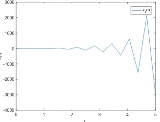
Figure 1 shows the behavior of the trajectories and their mean-square curve (green color) when ∆ = 0.004. Figure 2 shows one trajectory in this case. Figure 3 and Figure 4 illustrate that the numerical solution is mean-square stable when ∆ = 0.01 and ∆ = 0.001, respectively. In these figures, the stepsize ∆ is less than the constrained stepsize ∆∗= 0.01176. However, when ∆ = 0.3>∆∗, Figure 5 shows that the mean-square curve does not tend to zero, as shown in Figure 5, and the trajectory is unstable, as shown in Figure 6. Based on the simulations, we can see that the numerical solution is mean-square stable under the constrained stepsize proposed by Theorem 2.

Figure 1. Mean square stability of EM numerical solutionXkwith ∆ = 0.004.

0 1 2 3 4 5

t_n -0.1

0 0.1 0.2 0.3 0.4 0.5 0.6 0.7 0.8 0.9

x(t)

x

1(t)

Figure 3. Mean square stability of EM numerical solutionXk with ∆ = 0.01.

Figure 4. Mean square stability of EM numerical solutionXkwith ∆ = 0.001.

6

Conclusion

We investigated the almost sure exponential stability and the mean-square exponential stability of the trivial solution and the numerical solution for NSFDEs with jumps. By using the stochastic inequality and the semi-martingale convergence theorem, we proved that the numerical solution of the EM method can reproduce the corresponding stability of the trivial solution when the drift coefficient satisfies an additional condition. We generalized the existing stability results of the numerical solution to NSFDEs with jumps.

Acknowledgements This work was supported by the National Natural Science Foundation of China under Grants 61573156, 61503142, and the Key Youth Research Fund of Guangdong University of Technology under Grant 17ZK0010.

Conflict of interest The authors declare that they have no conflict of interest.

References

1 Kolmanovsky V B, Nosov V R. Stability of neutral-type functional differential equations. Nonlinear Anal-Theor, 1982, 6(9): 873–910

2 Mao X R. Exponential stability in mean square of neutral stochastic differential functional equations. Sys Control Lett, 1995, 26(4): 245–251

3 Mao X R. Razumikhin-type theorems on exponential stability of neutral stochastic differential equations. SIAM J Math Anal, 1997, 28(2): 389–401

4 Hu R. Asymptotic properties of several types of neutral stochastic functional differential equations. Ph.D. thesis, Huazhong University of Science & Technology, Wuhan, China, 2009

0 1 2 3 4 5 t_n

-1 0 1 2 3 4 5 6 7

x(t)

×106

E(|x(t)|2₎

Figure 5. Mean square stability of EM numerical solutionXkwith ∆ = 0.3.

0 1 2 3 4 5

t_n -4000

-3000 -2000 -1000 0 1000 2000 3000

x(t)

x

1(t)

Figure 6. A sample path of EM numerical solutionXkwith ∆ = 0.3.

6 Jankovi´c, S., Jovanovi´c, M. Thepth moment exponential stability of neutral stochastic functional differential equations. Filomat, 2006, 20(1): 59–72

7 Luo Q, Mao X R, Shen Y. New criteria on exponential stability of neutral stochastic differential delay equations. Sys Control Lett, 2006, 55(10): 826–834

8 Mao X R. Asymptotic properties of neutral stochastic differential delay equations. Stochastics: An International Journal of Probability and Stochastic Processes, 2000, 68(3-4): 273–295

9 Jiang F, Shen Y, Wu F K. A note on order of convergence of numerical method for neutral stochastic functional differential equations. Commun Nonlinear Sci, 2012, 17(3): 1194–1200

10 Yu Z H. The improved stability analysis of the backward Euler method for neutral stochastic delay differential equations. Int J Comput Math, 2013, 90(7): 1489–1494

11 Yu Z H. Almost sure and mean square exponential stability of numerical solutions for neutral stochastic functional differential equations. Int J Comput Math, 2015, 92(1): 132–150

12 Zong X F, Wu F K, Huang C M. Exponential mean square stability of the theta approximations for neutral stochastic differential delay equations. J Comput Appl Math, 2015, 286: 172–185

13 Wu F K, Mao X R. Numerical solutions of neutral stochastic functional differential equations. SIAM J Numer Anal, 2008, 46(4): 1821–1841

14 Wu F K, Mao X R, Szpruch L. Almost sure exponential stability of numerical solutions for stochastic delay differential equations. Numer Math, 2010, 115(4): 681–697

15 Li Q Y, Gan S. Almost sure exponential stability of numerical solutions for stochastic delay differential equations with jumps. J Appl Mathe Comput, 2011, 37(1-2): 541–557

16 Wu F K, Mao X R, Kloeden P E. Almost sure exponential stability of the Euler-Maruyama approximations for stochastic functional differential equations. Random Operators and Stochastic Equations, 2011, 19(2): 165–186 17 Tan J G, Wang H L, Guo Y F. Existence and uniqueness of solutions to neutral stochastic functional differential

equations with Poisson jumps. Abstr Appl Anal, 2012, vol. 2012, Article ID 371239

18 Liu D Z, Yang G Y, Zhang W. The stability of neutral stochastic delay differential equations with Poisson jumps by fixed points. J Comput Appl Math, 2011, 235(10): 3115–3120

19 Tan J G, Wang H L, Guo Y F, et al. Numerical solutions to neutral stochastic delay differential equations with Poisson jumps under local Lipschitz condition. Math Probl Eng, 2014, vol. 2014, Article ID 976183

21 Mo H Y, Zhao X Y, Deng F Q. Exponential mean-square stability of the θ-method for neutral stochastic delay differential equations with jumps. Int J Syst Sci, 2017, 48(3): 462–470

22 Zhu Q X. Asymptotic stability in thepth moment for stochastic differential equations with L´evy noise. J Math Anal Appl, 2014, 416(1): 126–142

23 Mao W, You S R, Mao X R. On the asymptotic stability and numerical analysis of solutions to nonlinear stochastic differential equations with jumps. J Comput Appl Math, 2016, 301: 1–15

24 Higham D, Mao X R, Yuan C G. Almost sure and moment exponential stability in the numerical simulation of stochastic differential equations. SIAM J Numer Anal, 2007, 45(2): 592–609

25 Tan J G, Wang H L. Mean-square stability of the Euler-Maruyama method for stochastic differential delay equations with jumps. Int J Comput Math, 2011, 88(2): 421–429

26 Zhou S B, Xie S F, Fang Z. Almost sure exponential stability of the backward Euler-Maruyama discretization for highly nonlinear stochastic functional differential equation. Appl Math Comput, 2014, 236: 150-160