A finite element approach to modelling fractal ultrasonic transducers

doi: 10.1093/imamat/dri017

A Finite Element Approach to Modelling Fractal Ultrasonic Transducers

EBRAHEMA. ALGEHYNE ANDANTHONYJ. MULHOLLAND

Department of Mathematics and Statistics, University of Strathclyde, 26 Richmond Street, Glasgow, G1 1XH, UK.

[Received on 22 April 2014]

Piezoelectric ultrasonic transducers usually employ composite structures to improve their transmission and reception sensitivities. The geometry of the composite is regular with one dominant length scale and, since these are resonant devices, this dictates the central operating frequency of the device. In order to construct a wide bandwidth device it would seem natural therefore to utilize resonators that span a range of length scales. In this article we derive a mathematical model to predict the dynamics of a fractal ultrasound transducer; the fractal in this case being the Sierpinski gasket. Expressions for the electrical and mechanical fields that are contained within this structure are expressed in terms of a finite element basis. The propagation of an ultrasonic wave in this transducer is then analyzed and used to derive expressions for the non-dimensionalised electrical impedance and the transmission and reception sensitivities as a function of the driving frequency. Comparing these key performance measures to an equivalent standard (Euclidean) design shows some benefits of these fractal designs.

Keywords: finite element method, fractal, ultrasound, transducer, renormalisation

1 Introduction

Ultrasonic transducers are devices that convert electrical energy into mechanical vibration and con-versely can convert mechanical energy into an electrical signal ( Yang (2006); Hayward et al. (1984); Mulholland & Walker (2011)). These devices can be used to interrogate a medium by emitting a wave (electrical to mechanical) and then listening to the same wave after it has traversed the medium (mechan-ical to electr(mechan-ical). Piezoelectric ultrasonic transducers typ(mechan-ically employ composite structures to improve their transmission and reception sensitivities ( Hayward (1984); Orr et al. (2007)) and many biological species produce and receive ultrasound such as moths, bats, dolphins and cockroaches. The manmade transducers tend to have very regular geometry on a single scale whereas the natural systems exhibit a wide variety of intricate geometries often with resonators over a range of length scales ( M¨uller et al. (2006); M¨uller (2004); Miles & Hoy (2006); Chiselev et al. (2009); Eberl et al. (2000); Nadrowski et

al. (2008); Robert & G¨opfert (2002); Montero de Espinosa et al. (2005)). This allows these transducers

to operate over a wider frequency range and hence results in reception and transmission sensitivities with exceptional bandwidths. To assess the benefits of having transducers with such structures it would be useful to build mathematical models of them. One structure whose geometrical components consist of a range of length scales is a fractal. There have been a number of mathematical approaches which describe wave propagation in fractal media ( Kigami (2001); Falconer (2003); Giona (1996); Abdulbake & Mulholland (2003); Abdulbake et al. (2004)). This paper constructs a model of a fractal ultrasound transducer and then uses this model to compare its operational qualities with that of a standard (Eu-clidean) design. Previously this topic was examined using a finite differences approach ( Mulholland & Walker (2011)). Previously this topic was examined using a finite differences approach ( Mulholland & Walker (2011)) whereby each edge in the fractal lattice was modelled as a one dimensional piezoelectric

c

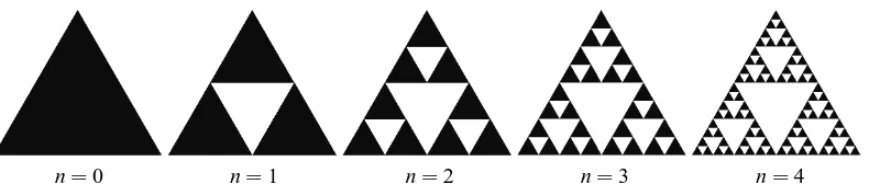
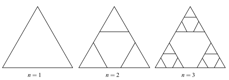
bar whose only degree of freedom was in the plane of the lattice. This model did not therefore allow for other types of motion of the lattice, or directions of the electric field, and was essentially a local de-scription of the dynamics of each edge that when joined to the other edges to form the lattice, led to the global dynamics of the device. This paper will derive the governing equations from the general tensor equations for the whole lattice so that the three dimensional world that the device is embedded within is accounted for. This framework allows different parameterisations to be deployed and in this paper we will examine the case where the displacement acts out of the plane of the lattice whereas the electric field operates within the plane of the lattice. This will allow us to consider the transverse modes of the device. In addition, this paper will be the first to use a finite element methodology as the basis for the renormalisation approach and it is precisely this global approach to modelling the device that permits this type of analysis. This renormalisation approach will be used in this paper to derive expressions for the key operational characteristics of the device. Of course, from a manufacturing respective only the pre-fractal (finite fractal generation level) gaskets can be feasibly constructed and so an investigation into the dependency of the device characteristics at a low fractal generation level is undertaken here. The fractal that will be used in this article to simulate this self-similar transducer is the Sierpinski gasket ( Falconer & Hu (2001)). Such an ultrasonic transducer would start with an equilateral triangle of piezo-electric crystal, and the next generation(n=1)would be obtained by replacing this by three copies of itself, each of which being half the size of the original triangle. This process is then repeated for several generations (see Figure 1). The Sierpinski gasket lattice of degree 3, SG(n)(3), is the lattice counterpart of the Sierpinski gasket ( Schwalm (1988)) (see Figure 2). This lattice is constructed by a process which starts from the Sierpinski gasket of order n=1 (which consists of three piezoelectric triangles), assigns a vertex to the centre of each of these triangles and, by connecting these vertices together with edges, the lattice at generation level n=1 (SG(1)_{(3)) is constructed. The lattice has side length L units which} remains constant as the generation level n increases. Therefore, as n increases, the length of the edge between adjacent vertices tends to zero and in this limit the lattice will perfectly match the space filling properties of the original Sierpinski gasket ( Mulholland (2008)). The total number of vertices is N=3n and h(n)=L/(2n₋1)is the edge length of the fractal lattice. The vertex degree is 3 apart from the boundary vertices (input/output vertices) which have degree 2 and M=3(3n₋1)/2 denotes the total number of edges. These boundary vertices will be used to interact with external loads (both electrical and mechanical) and so we introduce fictitious vertices A,B and C to accommodate these interfacial

boundary conditions (see Figures 3 and 4). Let us denote byΩ the set of points lying on the edges and vertices of SG(n)(3)and denote the region’s boundary by∂Ω.

n=0 n=1 n=2 n=3 n=4

n=1 n=2 n=3 FIG. 2. The first few generations of the Sierpinski gasket lattice SG(3).

2 Model Derivation

The lattice represents the vibrations of a piezoelectric material (the focus here is on PZT-5H Auld (1973)) that has been manufactured to form a Sierpinski gasket. The interplay between the electrical and mechanical behaviour of the lattice vertices is therefore described by the piezoelectric constitutive equations ( Yang (2006))

Ti j = ci jklSkl−eki jEk, (2.1)

Di = eiklSkl+εikEk, (2.2)

where Ti jis the stress tensor, ci jklis the stiffness tensor, Sklis the strain tensor, eki jis the piezoelectric tensor, Di is the electrical displacement tensor andεik is the permittivity tensor (where the Einstein summation convention is adopted). The strain tensor is related to the displacement gradients ui,j by Si j= (ui,j+uj,i)/2. The dynamics of the piezoelectric material is then governed by

ρTu¨i=Tji,j, (2.3)

subject to Gauss’ law

Di,i=0 (2.4)

whereρT is the density and uiis the component of displacement in the direction of the ithbasis vector. So, combining equations (2.3) and (2.1) gives

ρTu¨i=cjiklSkl,j−ek jiEk,j, (2.5) and combining equations (2.4) and (2.2) gives

Di,i=eiklSkl,i+εikEk,i=0. (2.6) In this paper attention is restricted to the out of plane displacement only (a horizontal shear wave) by stipulating that u= 0,0,u3(x1,x2,t)

of the vector elastodynamical equations. Now if E= E1(x1,x2),E2(x1,x2),0

then, for PZT-5H Auld (1973), equation (2.5) becomes

ρTu¨3=c44(u3,11+u3,22)−e24(E1,1+E2,2), (2.7) where the Voigt notation has been used to express these tensors as matrices. For example, c44≡c2323 and e24≡e223. Equation (2.6) gives

E1,1+E2,2=−

e24 ε11

(u3,11+u3,22), (2.8)

whereε22=ε11for PZT-5H. Combining these two equations gives ¨

u3=c2T∇2u3 (2.9)

where∇2= (∂2_/∂_x2

1+∂2/∂x22), cT = p

µT/ρT is the (piezoelectrically stiffened) wave velocity and µT =c44(1+e2₂₄/(ε11c44))is the piezoelectrically stiffened shear modulus, subject to the initial condi-tions u3(x,0) =u˙3(x,0) =0 and the boundary conditions of continuity of displacement and force at∂Ω. By introducing the non-dimensionalised variableθ=cTt/h, dropping the subscript on u, and applying the Laplace transformL :θ_→q gives

q2u=h2∇2u. (2.10)

Now seek a weak solution u_∈H1(Ω)where on the boundary u=u_{∂Ω ∈}H1(∂Ω).Multiplying by a test function w_∈H_B1(Ω), where H_B1(Ω):={w_∈H1(Ω): w=0 on∂Ω_},integrating over the regionΩ, and using Green’s first identity gives

Z

Ω(q

2_{u w+h}2_{∇u.∇w)dx=0. (2.11)}

3 Galerkin discretisation

Using a standard Galerkin method we replace H1(Ω)and H_B1(Ω)by the finite dimensional subspaces

S and SB=S∩HB1(Ω). Let UB∈S be a function that approximates u∂Ω on∂Ω, then the discretised problem involves finding U_∈S such that

Z

Ω(q

2_{U W+h}2_{∇U.∇W)dx=0, (3.1)}

where W is the test function expressed in this finite dimensional space. Let_{φ1,φ2,···,φN}form a basis of SBand set W =φj, then

Z

Ω(q

2_Uφ

j+h2∇U.∇φj)dx=0. (3.2)

Furthermore, letφI, I={N+1,N+2,N+3}form a basis for the boundary nodes and let

U= N

∑

Uiφi+

∑

UBiφi. (3.3)

Hence, equation (3.2) can be written as

where

b(_jn)=−

∑

Z

Ω(q

2_φ

iφj+h2∇φi.∇φj)dx

UBi, (3.5)

A(_jin)=q2H_ji(n)+h2K(_jin), (3.6)

K(_jin)= Z

Ω(∇φj.∇φi)dx, (3.7)

and

H(_jin)= Z

Ω(φjφi)dx. (3.8)

The lattice basis function at vertex x_jis chosen to be

φj(x,y) = (

a+bx+cy+d(x2_+y2_{) j∈ {1,···,N}}

a+d(x2_+y2_{) j∈I.} (3.9)

where(x,y)∈Ω and a,b,c,d_∈Rare coefficients to be determined. Futhermore, theφjare defined as localised basis functions such that

φj(x,y) = (

1 if(x,y) = (xj,yj)

0 if(x,y) =coordinates of vertices adjacent to vertex j, (3.10)

andφj(x,y) =0 at all points which do not lie in the edges adjacent to vertex j. For each generation level of the SG(n)(3) lattice the coordinates of the vertices are known. Using equation (3.10) the coefficients in equation (3.9) can be determined. For a particular element lying between vertex i and vertex j the isoparametric representation, given byx(s),y(s)=(xj−xi)s+xi,(yj−yi)s+yi

is employed, where

s1=0 and s2=1 and dx=hds. Substituting this into equation (3.7) gives for each element (edge) e where e=1,···,M

e_K(n)

ji = 4 h        R1

0s2ds =13 if j=i=p

R1

0s(s−1)ds =−16 if(j=p and i=q)or(j=q and i=p)

R1

0(s−1)2ds =13 if j=i=q

0 otherwise

(3.11)

where element e connects node p to node q. For the boundary elements e_{∈ {}M+1,M+2,M+3_} e_K(n)

ji = ₄

3h if j=i=q

0 otherwise , (3.12)

where q is the corner node of the SG(3)lattice connected to element e (for n=1, q_{∈ {}1,2,3_}, and for n=2, q_{∈ {}1,5,9_}). Equations (3.11) and (3.12) can then be used to assemble the full matrix in equation (3.7). Similarly, foreH(_jin)where e_{∈ {}1,···,M_}, equation (3.8) leads to

e_H(n)

ji =h        R1

0(s2−1)2ds =158 if j=i=p

R1

0(s2−1)(s−2)s ds =1130 if(j=p and i=q)or(j=q and i=p)

R1

0(s−2)2s2ds =158 if j=i=q

0 otherwise

1 2 3

A B

C

(0,0) (h,0)

(h/2,√3h/2)

(−h,0) (2h,0)

(h,√3h)

1

2

4

6

FIG. 3. The Sierpinski Gasket lattice SG(3)at generation level n=1. Nodes 1,2 and 3 are the input/output nodes, and nodes A,B and C are fictitious nodes used to accommodate the boundary conditions. The lattice has 6 elements (circled numbers), with two vertices adjacent to each element.

where element e connects node p to node q, and for the boundary elements e_{∈ {}M+1,M+2,M+3_}

e_H(n)

ji =h R1

0(s2−1)2ds =158 if j=i=q

0 otherwise (3.14)

where q is the corner node of the SG(3)lattice connected to element e. Combining equations (3.11),(3.12),(3.13) and (3.14) gives equation (3.6) as A(_ji1)=hα if j=i and hβ otherwise whereα=4+ (8q2/5),and β = (−2/3) +11q2_{/30.In general A}(n)

ji =A¯

(n−1)

ji +βV

(n)

ji , where ¯A

(n−1)

ji is a block diagonal matrix con-sisting of 3 copies of A(_jin−1)and V_ji(n)is the adjacency matrix for the subgraph of SG(n)(3) consisting of the edges that connect each of the three SG(n−1)(3) graphs. A similar treatment can be given to equation (3.5) to give (where m= (N+1)/2)

b(_jn)=

     

    

−(R eM+1(q

2φ

N+1φj+h2∇φN+1.∇φj)dx)UA, j=1 −(R

eM+2(q

2φ

N+2φj+h2∇φN+2.∇φj)dx)UB, j=m −(R

eM+3(q

2_φ

N+3φj+h2∇φN+3.∇φj)dx)UC, j=N

0 otherwise

1 2 3 4 5 6 7 8 9 A B C replacements

(0,0) (h,0) (h/2,√3h/2)

(2h,0) (3h,0) (5h/2,√3h/2) (h,√3h) (2h,√3h)

(3h/2,3√3h/2)

(−h,0) (4h,0)

(2h,2√3h)

1 2 3 4 5 6 7 8 9 10 11 12 13 14 15

FIG. 4. The Sierpinski Gasket lattice SG(3)at generation level n=2. Nodes A,B and C are fictitious nodes used to accommodate the boundary conditions. The lattice has 15 elements (circled numbers), with two vertices adjacent to each element.

Using the isoparametric representation given above

b(_jn)=

          

hη(_jn)UA, j=1 hη(_jn)UB, j=m hη(_jn)UC, j=N

0 otherwise

(3.16)

where

η(n)

j =

(₄ 3−

2 15q

2_{, j=1}

1+ 1

3(2n+1₋₁₎+

(11−15×2n₎ 30(2n+1₋₁₎q

2_{, j=m or N.} (3.17)

3.1 Application of the Mechanical boundary conditions

Mechanical and electrical loads are now introduced to the transducer at its boundaries. It can be shown that ( Algehyne & Mulholland (2014))

Ui=G(_jin)δ¯j

(n)

, (3.18)

Here ˆA=A/h,

ˆ

B(_jin)=

( ˆ γ(n)

j , j=i

0 otherwise, (3.19)

ˆ γ(n)

j =η

(n)

j γjand ˆδ

(n)

j =η

(n)

j δj, where

γj=   

 

(1₋qZB ZT)

−1_{, j=1}

(1₋qZL ZT)

−1_{, j=m or N}

0 otherwise

(3.20)

and

δj=         

−_µζ_TQ_ξ1₋qZB ZT

−1

, j=1

1₋qZL

ZT −1_ζ

Q

µTξ −2ALq ZL ZT

, j=m or N

0 otherwise,

(3.21)

where the mechanical impedance of the load is ZL=ρLcLAr, and of the backing material is ZB=ρBcBAr, and of the transducer is ZT=ρTcTAr, whereρL(ρB) is the density and cL(cB) is the wave velocity in the load (backing material). Alsoζ=e24/ε11, and Q is the electrical charge applied at one of the transducer-electrical load interfaces. At each generation level of the Sierpinski gasket transducer the ratio of the cross-sectional area of each edge to its length is denoted byξ =Ar/h. The overall extent of the lattice (L)is fixed and so the length of the edges will steadily decrease and, by fixingξ, the cross-sectional area will also decrease as the fractal generation level increases (in fact Ar=ξL/(2n−1)).

4 Renormalisation

From equation (3.18) the desired weightings at each vertex inΩ is given by

U_j(n)=G(_j1n)δˆ₁(n)+G(_jmn)δˆm(n)+G(jNn)δˆ

(n)

N . (4.1)

It will transpire later that only U₁(n),Um(n)and UN(n)are required and so only the pivotal Green’s functions G(_{i j}n), i,j_{∈ {}1,m,N_}need to be calculated. Temporarily ignoring matrix ˆB (this matrix originates from

consideration of the boundary conditions) then, due to the symmetries of the SG(3)lattice (and hence in matrix A(n)_{), ˆG}(n)

ii =Gˆ

(n)

j j =xˆ, say, where i,j∈ {1,m,N} (that is, corner-to-same-corner), and ˆ

G(_jkn)=Gˆ_hk(n)=yˆ, say, where j,k,h_{∈ {}1,m,N_}, j₆=k₆=h (that is, corner-to-other-corner), where

ˆ

G(n)= (_Aˆ(n)₎−1_{. (4.2)}

At level n+1, we denote, ˆX =_Gˆ(n+1)

ii and ˆY =Gˆ

(n+1)

1

b

e

m

d

q

r

z

N

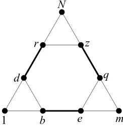
FIG. 5. Three Sierpinski Gasket lattices of generation level n−1 (SG(n−1)(3)) are connected by the edges in bold (d,r),(b,e) and(q,z)

to create the Sierpinski Gasket lattice at generation level n (SG(n)_(3)).

one must ensure that the frequency is scaled appropriately (by(cT/h(n))−1) when re-dimensionalising. An iterative procedure can be developed from equation (3.6) to give ( Algehyne & Mulholland (2014))

G(n)=_Gˆ(n)_+Gˆ(n)_Bˆ(n)_G(n)_{. (4.3)} The system of linear equation will create the renormalisation recursion relationships for the pivotal Green’s functions. Since the subgraphs of Figure 5 only connect to each other at the corners, it will transpire that the recursions in equation (4.3) only involve two pivotal Green’s functions, namely, corner-to-corner and corner-to-same-corner; the so called input/output nodes. Solving these (for ˆy₆=0,β 6=0) gives

ˆ

X=x+ˆ 2β

2_yˆ2_(xˆ+βˆx2_−βyˆ2₎

(1+βˆx+βy)(ˆ 1₋β2_xˆ2₋β_yˆ+β2_yˆ2₎, (4.4) and

ˆ

Y= −βyˆ

2₍₁₊β_ˆx−β_y)ˆ

(1+βˆx+βˆy)(1₋β2_xˆ2₋β_yˆ+β2_yˆ2₎. (4.5) The boundary conditions can now be re-introduced and lead to

x=xˆ+2 ˆy ˆγmy

1₋ˆx ˆγ1

, (4.6)

y= yˆ

1₋ˆx ˆγ1 1−γˆm(xˆ+y)ˆ−2 ˆy2γˆ1γˆm

, (4.7)

z=xˆ+ˆy ˆγ1y+ˆy ˆγmr

1₋ˆx ˆγm

, (4.8)

and

r= y 1ˆ +γˆ1y(1+γˆm(yˆ−x))ˆ

(x ˆˆγm−1+ˆy ˆγm)(x ˆˆγm−1−ˆy ˆγm)

, (4.9)

5 Electrical Impedance and Transmission and Reception Sensitivity

The derivation of the operating characterstics of the device follows similar lines as presented in (Mulhol-land & Walker (2011)) and so is omitted (a full derivation is given in (Algehyne & Mulhol(Mulhol-land (2014))). The non-dimensionalised electrical impedance is given by

ˆ

ZE(f ; n) =ZE/Z0=

Z_T

C0qµTξZ0

1+ζ

2_C 0 µTξ

(σ1+σ2)

(5.1)

whereσ1= 1−q(ZB/ZT) −1

η(n) 1 (G

(n)

N1−G

(n)

11)andσ2= 1−q(ZL/ZT) −1

η(n)

m (−G(Nmn)−G

(n)

NN+2G

(n) 1N) and Z0is the series electrical load. The non-dimensionalised transmission sensitivityψ is given by

ψ(f ; n) =F V

/ζC0=

aZL (ZE+b)µTξC0

K(n), (5.2)

where

K(n)=1₋qZL ZT

−1

−η1(n)

1₋qZB ZT

−1

G(_m1n)+ηm(n)

1₋qZL ZT

−1

(G(mmn)+G(_mNn)) +1

. (5.3)

The non-dimensionalised reception sensitivityφis

φ(f ; n) = V F

(e24L)

= 2ζe24Lσ2 ξ µT

1₋ζ

2_aZ

T(σ1+σ2)

(ZE+b)qµT2ξ2

−_(Z aZT E+b)qµTξC0

−1

. (5.4)

Having derived expressions for the main operating characteristics of this new device it is instructive to compare these with a model of a standard device ( Hayward (1984); Hayward et al. (1984)) to assess any practical benefits arising from this novel design.

6 Numerical Results For Pre-Fractal Ultrasound Transducers

From a practical perspective, these fractal transducers will only be able to be manufactured at low gen-eration levels. Indeed some preliminary work to manufacture this fractal design at gengen-eration level

assessment can be made at an earlier stage by connecting the transducer to an electrical circuit and mea-suring its electrical impedance over a range of frequencies. A typical profile of this electrical impedance spectrum (magnitude) given by equation (5.1) is shown in Figure 6 (dashed line); it is compared to the equivalent profile given by a model of the traditional design (full line) (Hayward et al. (1984)). The overall trend of the curve is that of a capacitor (1/f profile) with a series of resonances. The important

2 4 6 8 10 30

35 40 45

f (MHz) |ZE(f ; n)|(dB)

FIG. 6. Non-dimensionalised electrical impedance (equation (5.1)) versus frequency for the SG(3)lattice transducer at fractal generation level n=3 (dashed line). The non-dimensionalised electrical impedance of the standard (Euclidean) transducer is plotted for comparison (full line). Parameter values are given in (Auld (1973)) for PZT-5H.

2 4 6 8 10

-20 -10

10 20 30 40

f (MHz) |ψ(f ; n)|(dB)

2 4 6 8 10

-30 -20 -10

10 20

f (MHz) |φ(f ; n)|(dB)

FIG. 8. Non-dimensionalised reception sensitivity (equation (5.4)) versus frequency for the SG(3)lattice transducer at fractal generation level n=3 (dashed line). The non-dimensionalised reception sensitivity of the standard (Euclidean) transducer is plotted for comparison (full line). Parameter values are given in (Auld (1973)) for PZT-5H.

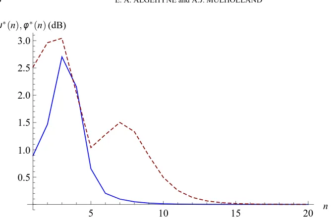
The convergence of the device’s operating characteristics as the fractal generation level increases can be examined. To do this the norm of the difference between the energy in the power spectrum at succes-sive generation levels, integrated with respect to frequency, is calculated for the transmission/reception sensitivities, as follows

m

∑

|ψ(fi; n)−ψ(fi; n+1)|=ψ∗(n), (6.1)

and

m

∑

|φ(fi; n)−φ(fi; n+1)|=φ∗(n). (6.2)

5 10 15 20 0.5

1.0 1.5 2.0 2.5 3.0

n ψ∗_(n),φ∗_(n)(dB)

FIG. 9. The convergence of the transmission and reception sensitivities is examined by plotting the differences in the energies in successive spectra as the fractal generation level increases. Non-dimensionalised transmission sensitivity(ψ∗(n))(equation (6.1)) (full line) and non-dimensionalised reception sensitivity (φ∗(n)) (equation (6.2)) (dashed line) versus the fractal generation level. The transmission sensitivity converges by generation level n=10 and the reception sensitivity by generation level n=16, over this frequency range where fi∈[0.1,10]MHz.

Design Parameter Symbol Magnitude Dimensions

Parallel electrical impedance load ZP 1000 Ohms

Series electrical impedance load Z0 50 Ohms

Length of transducer L 1 mm

Mechanical impedance of the front load ZL 1.5 MRayls

Mechanical impedance of the backing layer ZB 2 MRayls

Wave speed in the front load cL 1500 ms−1

Wave speed in the backing layer cB 1666 ms−1

Density of the front load ρL 1000 kgm−3

Density of the backing layer ρB 1200 kgm−3

Table 1. Parameter Values for the Sierpinski Gasket Transducer ( Mulholland et al. (2007); Mulholland & Walker (2011)). For PZT-5H parameters see (Auld (1973))

.

7 Conclusions

Acknowledgements

The authors gratefully acknowledge the support given by the Ministry of Higher Education, University of Tabuk in Saudi Arabia and the Royal Embassy of Saudi Arabia in UK.

References

ABDULBAKE, J., MULHOLLAND, A. J. & GOMATAM, J. (2004) Existence and Stability of Reaction-Diffusion Waves on a Fractal Lattice, Chaos, Solitons and Fractals, 20(4), 799–814.

ABDULBAKE, J., MULHOLLAND, A. J.& GOMATAM, J. (2003) A Renormalization Approach To Reaction-Diffusion Processes On Fractals, Fractals, 11(4), 315–330.

ALGEHYNE, E. A. & MULHOLLAND, A. J. (2014) A Finite Element Approach to Modelling Fractal Ultrasonic Transducers, Department of Mathematics and Statistics, University of Strathclyde,

Depat-mental report, 35(1).

AULD, B. A. (1973) Acoustic Fields and Waves in Solids, New York, John Wiley and Sons, 1. BARLOW, M. T. (1998) Diffusion on fractals, Lectures on Probability Theory and Statistics, Berlin: Springer, ed P Bernard, (Lecture Notes in Mathematics vol (1690)), 1–121.

CHISELEV, A. M., MORARU, L. & GOGU, A. (2009) Localization of an object using a bat model inspired from biology, Romanian, J. Biophys, 19(4), 251–258.

DERFEL, G., GRABNER, P. J. & VOGL, F. (2012) Laplace operators on fractals and related functional equations, J. Phys. A: Math. Theor., 45(463001), doi:10.1088/1751-8113/45/46/463001. EBERL, D. F., HARDY, R. W. & KERNAN, M. J. (2000) Genetically similar transduction mechanisms for touch and hearing in Drosophila, J. Neurosci, 20(16), 5981–5988.

FALCONER, K. (2003) Fractal Geometry: Mathematical Foundations and Applications, Chichester, England John Wiley and Sons Ltd,.

FALCONER, K. & HU, J. (2001) Nonlinear Diffusion Equations on Unbounded Fractal Domains, J

Math Anal App, 256, 606–624.

GIONA, M. (1996) Transport Phenomena in Fractal and Heterogeneous Media: Input/Output Renor-malization and Exact Results Chaos, Solitons and Fractas, 7(9), 1371–1396.

GIONA, M., SCHWALM, W.A., SCHWALM, M.K. & ADROVER, A. (1996) Exact solution of linear transport equations in fractal media – I. Renormalization analysis and general theory, Chem.

Eng. Sci, 51(20), 4717–4729.

HAYWARD, G. (1984) A systems feedback representation of piezoelectric transducer operational impedance, Ultrasonics, 22, 153–162.

HAYWARD, G., MCLEOD, C. J. & DURANNI, T. S. (1984) A systems model of the thickness mode piezoelectric transducer, JASA, 76(2), 369–382.

MILES, R. N.& HOY, R. R. (2006) The development of a biologically-inspired directional microphone for hearing aids, Audiol Neurootol, 11(2), 86-94.

MONTERO DEESPINOSA, F., MARTINEZ, O., SEGURA, L.E. & GOMEZ-ULLATE, L. (2005) Double frequency piezoelectric transducer design for harmonic imaging purposes in NDT, IEEE. TUFFC,

52(6), 980–986.

MULHOLLAND, A. J. (2008) Bounds on the Hausdorff dimension of a renormalisation map arising from an excitable reaction-diffusion system on a fractal lattice, Chaos, Solitons and Fractals, 35(2), 274–284.

MULHOLLAND, A. J. & WALKER, A. J. (2011) Piezoelectric Ultrasonic Transducers With Fractal Geometry, Fractals, 19(4), 469–479.

MULHOLLAND, A. J., RAMADAS, N., O’LEARY, L., PARR, A.C. S., TROGE, A., HAYWARD, G. & PETHRICK, R. A. (2007) A Theoretical Analysis of a Piezoelectric Ultrasound Device with an Active Matching Layer, Ultrasonics, 47(1), 102–110.

MULHOLLAND, A. J., WALKER, A. J., MACKERSIE, J. W., O’LEARY, R. L., GACHAGAN, A. & RAMADAS, N. (2011) The Use of Fractal Geometry in the Design of Piezoelectric Ultrasonic Trans-ducers, Ultrasonics Symposium (IUS), 2011 IEEE International, 1559–1562.

M ¨ULLER, R. (2004) A numerical study of the role of the tragus in the big brown bat, JASA, 116(6), 3701–3712.

M ¨ULLER, R., LU, H., ZHANG, S. & PEREMANS, H. (2006) A helical biosonar scanning pattern in the chinese noctule Nycatalus plancyi, JASA, 119(6), 4083–4092.

NADROWSKI, B., ALBERT, J. T. & G ¨OPFERT, M. C. (2008) Transducer-Based Force Generation Explains Active Process in Drosophilia Hearing, Curr. Biol, 18, 1365–1372.

ORR, L. A., MULHOLLAND, A. J., O’LEARY, R. L., PARR, A., PETHRICK, R. & HAYWARD, G. (2007) Theoretical modelling of frequency dependent elastic loss in composite piezoelectric transduc-ers, Ultrasonics, 47(1), 130–137.

ROBERT, D.& G ¨OPFERT, M. C. (2002) Novel schemes for hearing and orientation in insects, Curr.

Opin. Neurobiol, 12, 715–720.

SCHWALM, W. A. & SCHWALM, M. K. (1988) Extension theory for lattice Green functions,

Phys.Rev.B, 37(16), 9524–9542.

YANG, J. (2006) The Mechanics of Piezoelectric Structures, Singapore, World Scientific,. YANG, J. (2006) Analysis of Piezoelectric Devices, Singapore, World Scientific,.

Nomenclature

Notation Description

A,B,C The boundary vertices in the SG(n)(3)lattice

A(_jin) One of the matrices used to construct G(_jin)(see equation (3.6)) ¯

A(_jin−1) The block diagonal matrix consisting of 3 copies of A(_jin−1) ˆ

A(_jin) A(_jin)/h

Ar The cross-sectional area of each edge of the fractal lattice Ar=ξL/(2n−1) AL Amplitude of pressure wave incident on the transducer during reception mode a ZP/(Z0+ZP)

ˆ

B(_jin) One of the matrices used to create G(_jin)(see equation (3.19))

b Z0ZP/(Z0+ZP)

b(_jn) A vector arising from the boundary conditions (see equation (3.5))

C0 The capacitance of the transducer

ci jkl The stiffness tensor of the piezoelectric material

cT The (piezoelectrically stiffened) wave velocity in the SG(n)(3)lattice cL Wave speed in the front load

cB Wave speed in the backing layer Di The electrical displacement tensor Ei The electric field vector

eki j The piezoelectric tensor of the piezoelectric material e An element (edge) in SG(n)(3)

F The force on the boundary of the transducer ˆ

f(n) The non-dimensionalised natural frequency

G(_jin) The Green’s transfer matrix ˆ

G(n) Gˆ(n)= (_Aˆ(n)₎−1_{(see equation (4.2))}

h(n) _{The edge length of the fractal lattice L/(2}n₋₁₎

H1(Ω) Sobolev space of order 1 in domainΩ

H1(∂Ω) Sobolev space of order 1 at the boundary∂Ω

H_B1(Ω) Sobolev space of order 1 in domainΩ where the functions are zero on the boundary

H(_jin) A matrix used to construct A(_jin)(see equation (3.8))

I The set of vertices at the boundaries of SG(n)(3) K(_jin) A matrix used to construct A(_jin)(see equation (3.7))

L Length of transducer

M The total number of edges in the SG(n)(3)lattice

m The vertex labelled(N+1)/2

N=3n The total number of vertices in the SG(n)(3)lattice

n The fractal generation level

n The outward pointing unit normal from the edge element dr

Q The electrical charge applied to the boundary of the transducer

Notation Description

SG(n)(3) The Sierpinski gasket lattice of degree 3

Skl The strain tensor

S The finite dimensional subspace correspondury to H1(Ω) SB The finite dimensional subspace correspondury to HB1(Ω)

s The parameter used in the isoparametric description of each element

Ti j The stress tensor

t Time

ui,j The displacement gradients

ui The component of displacement in the direction of the ithbasis vector u_∂Ω The displacement in the boundary of SG(n)(3)

UB The function that approximates the displacement at the boundary U The approxmate displacement in regionΩ (see equation (3.3)

UBi The displacement at the boundary vertex Bi

UA,UB,UC The displacement of the boundary vertices{A,B,C}

V_ji(n) The adjacency matrix for the subgraph of SG(n)(3) consisting of the edges that connect each of the three SG(n−1)_{(3) graphs}

V The voltage applied to the transducer

W The test function in the finite dimensional space SB, W =φj w The test function in the infinite dimensional weak formulation

r r=G(_mNn)

ˆ

X Xˆ =_Gˆ(n+1)

ii where i∈ {1,m,N} x The spatial coordinates (cartesian)

x_j The spatial location of vertex j in the SG(n)_(3)lattice

x x=G(₁₁n)

ˆ

x xˆ=_Gˆ(n)

ii =Gˆ

(n)

j j where i,j∈ {1,m,N} ˆ

Y Yˆ =_Gˆ(n+1)

i j where i,j,∈ {1,m,N},i6=j y y=G(_1mn)=G(_1Nn)

ˆ

y yˆ=Gˆ_ik(n)=Gˆ(_hkn)where j,k,h_{∈ {}1,m,N_}, j₆=k₆=h ZB Mechanical impedance of backing layer

ZL Mechanical impedance of the front load ZT Mechanical impedance of the transducer ZP Parallel electrical impedance load Z0 Series electrical impedance load

ˆ

Notation Description

α Non-dimensionalised parameter given by equation (3.14) β Non-dimensionalised parameter given by equation (3.14) γj Non-dimensionalised parameter given by equation (3.20)

ˆ γ(n)

j η

(n)

j γj

δj Non-dimensionalised parameter given by equation (3.21) ˆ

δj

(n)

η(n)

j δj

εik The permittivity tensor ζ e24/ε11

η(n)

j Non-dimensionalised parameter given by equation (3.17) θ The non-dimensionalised temporal variable

µT The (piezoelectrically stiffened) shear modulus

ξ Ar/h

ρB Density of the backing layer ρL Density of the front load

ρT The density of the piezoelectric material φj The localised basis function at vertex j φ(f ; n) The non-dimensionalised reception sensitivity

φ∗_{(n) The reception sensitivity integrated over all frequencies}

ψ(f ; n) The non-dimensionalised transmission sensitivity

ψ∗_{(n) The transmission sensitivity integrated over all frequencies}

Ω The set of points lying on the edges and vertices of SG(n)(3)

∂Ω The region’s boundary

ˆ