Design optimization framework to estimate environmental impact of design decisions in consumer products

Rochester Institute of Technology

RIT Scholar Works

Theses Thesis/Dissertation Collections

2-2012

Design optimization framework to estimate

environmental impact of design decisions in

consumer products

Carlos M. Briceno

Follow this and additional works at:http://scholarworks.rit.edu/theses

This Thesis is brought to you for free and open access by the Thesis/Dissertation Collections at RIT Scholar Works. It has been accepted for inclusion in Theses by an authorized administrator of RIT Scholar Works. For more information, please [email protected].

Recommended Citation

Design optimization framework to estimate environmental

impact of design decisions in consumer products

by

Carlos M. Briceño

A thesis submitted to the graduate faculty of

Rochester Institute of Technology in partial

fulfillment of the requirements for the degree of

Master of Science

Industrial and Systems Engineering

Rochester, NY

March 2012

APPROVED BY

_______________________ __________________

Dr. Andres L. Carrano Dr. Brian K. Thorn

Industrial and Systems Engineering Industrial and Systems Engineering

Chair of Advisory Committee

_______________________ Dr. Marcos Esterman

1

Abstract

Most products have the potential to negatively impact the environment during all life-cycle stages. However, most environmental impact assessment methods focus on a single product life-cycle and on a specific lifecycle stage. In addition, consumer products can potentially amplify these impacts with their larger production volumes, wide dispersion, and miniaturization trends. The main objective of this project is to develop a design optimization framework that allows for estimating the environmental impact of design decisions (e.g. materials choice, etc.) across all life-cycle stages in consumer products. This work incorporates into one framework customer preferences (including preference for environmental friendliness), consumer adoption translated into utility for the producers, and environmental impact quantification of design options. The methodology relies on QFD, multi-attribute utility theory, non-linear mathematical programming, and Lifecycle Assessment tools to estimate the utility of the design options to the customer, the producer, and the environment. A function that depicts the utility of design perceived by the environment is introduced. Also a “Global Utility” equation is introduced. It incorporates the utilities of all three stakeholders and reflects the overall utility of the design alternatives.

2

Table of Content

Abstract ... 1

1. Background ... 6

2. Problem Statement ... 13

3. Literature Review ... 18

4. Methodology ... 23

4.1. Voice of customer and QFD ... 25

4.2. Design Utility Perceived by the Customer ... 29

4.3. Design Utility Perceived by the Producer ... 34

4.4. Design Utility Perceived by the Environment ... 38

4.5. Global Utility ... 43

5. Case Study ... 46

5.1. Voice of the Customer and Quality Function Deployment ... 46

5.2. Utility Perceived by Customer ... 56

5.3. Utility Perceived by Producer ... 67

5.4. Utility Perceived by the Environment ... 68

5.5. Global utility ... 80

5.6. Flexing the Model ... 81

5.7. Redesign of existing product ... 85

5.8. Sensibility analysis ... 94

6. Conclusions ... 97

7. Future work ... 99

8. Bibliography ... 100

9. APPENDICES ... 105

9.1. APPENDIX I: Assessment of Utility Function ... 105

9.2. APENDIX II: Scaled Pair Comparison ... 110

3

List of Figures

Figure 1-1 Product life cycle………..……… 10

Figure 2-1 Gap between actual and perceived environmental impact. ………. 14

Figure 2-2 Problem scheme………...……… 17

Figure 4-1 High level view of the proposed framework……… 24

Figure 4-2 QFD linked matrices……… 25

Figure 4-3 A matrix II is developed per available design option………...… 26

Figure 4-4 Detailed framework for step 1:Voice of Customer and QFD………..……… 28

Figure 4-5 Interpretation of house Ii with respect to optimization model……….……… 29

Figure 4-6 Lottery questions……….……… 30

Figure 4-7 Detailed framework for step 2: Customer’s Utility…...…..……… 33

Figure 4-8 Logit model coefficients………... 36

Figure 4-9 Detailed framework for step 3: Producer’s Utility……….. 37

Figure 4-10 Family of curves depicted by the utility function of the environment. ………. 39

Figure 4-11 Scaling of the utility function of the planet. ………..……… 40

Figure 4-12 Detailed framework for step 4: Planet’s Utility…….……… 42

Figure 4-13 Detailed framework for step 5: Global Utility……..……….……… 45

Figure 5-1 House of quality………...……… 48

Figure 5-2 Example of the two cases……….……… 49

Figure 5-3 Solar lamp house II………..……… 53

Figure 5-4 Low volt lamp house II……… 54

Figure 5-5 Utility function for lamp efficiency………. 58

Figure 5-6 Utility functions resulted from iteration process………..……… 59

4

Figure 5-8 Transformer and low voltage lamp parts and packaging……….……… 69

Figure 5-9 Solar lamp bill of materials……….… 70

Figure 5-10 Low voltage lamp bill of materials ………... 71

Figure 5-11 Materials and process input in Simapro for solar lamp. ……….. 73

Figure 5-12 Materials and process input in Simapro for low voltage lamp……….. 74

Figure 5-13 Simapro assessment output for solar lamp……… 76

Figure 5-14 Simapro assessment output for low voltage lamp………. 77

Figure 5-15 Comparison of environmental impact between low voltage and solar lamp………. 78

Figure 5-16 Planet utility function with I = 0.2………. 79

Figure 5-17 Response surfaces for solar and low voltage lamp respect to the weight factors……….. 84

Figure 5-18 Line of equal global utility for solar and low voltage lamps………. 84

Figure 5-19 Materials and process input in Simapro. ……….. 89

Figure 5-20 Comparison of environmental impact between lamp with aluminum and abs pole 90 Figure 5-21 Simapro assessment output for lamp with aluminum pole……… 91

Figure 5-22 Simapro assessment output for lamp with ABS pole……….…… 92

Figure 5-23 Response surfaces for lamps with aluminum and ABS pole………. 94

Figure 9-1 Lottery question to assess scaling constant ai for weight……….…….…… 107

5

List of tables

Table 5-1 Scale Pair Comparison ... 47  

Table 5-2 Comparison between low-voltage and solar lamps ... 51  

Table 5-3 Preferences between certain performance level and probabilities of best and worst performance levels ... 57  

Table 5-4 Utility function points ... 57  

Table 5-5 Lottery question for scaling constant x1 ... 60  

Table 5-6 Scaling constant a1 ... 61  

Table 5-7 Materials and processes inventory for solar and low voltage lamps ... 72  

Table 5-8 Higher global utility among design option based on design tendency ... 83  

Table 5-9 Monte Carlo sensibility simulation with upper and lower limits of xi ... 95  

Table 5-10 Monte Carlo sensibility simulation with ±10% of optimal xi values. ... 95  

Table 5-11 Monte Carlo sensibility simulation with random set of attributes with Uc= 0.8 ... 96  

6

1.

Background

From the beginnings of civilization humans have adapted to the surrounding environment modifying it to guarantee the survival and later to make their lifestyle more convenient and comfortable. Most of these changes brought positive impacts to their lives but perhaps not to the environment. Furthermore, during the industrial age the capacity to transform the environment accelerated dramatically. Mass production brought the capacity to satisfy the needs of a constantly growing population, but also required a large amount of resources generating a larger impact to the environment. Also, waste became an important issue. Some of the significant impacts caused to the environment are the release of large amount of greenhouse gases, the discharge of toxic residues into natural water bodies, the deforestation, and the alteration of large areas of land to acquire raw materials or housing spaces among others.

Carew and Mitchell (2002) stated that “humans have attained the unprecedented capacity to modify the natural environment on a global scale, and with this capacity comes the need for a new type of responsibility”. Anthropogenic activities are pressuring every natural system on the planet; many systems are disintegrating under these mounting pressures (UNEP, 2002). Some of the disturbing trends cited by the United Nations Environmental Program’s report include:

• 2.8 billion people live on less than $2 per day; 1.2 billion of these subsist on less

than $1 per day

• approximately 1.1 billion people lack access to safe drinking water

• approximately half of the planet’s rivers are seriously depleted and polluted

• approximately 24% of mammals and 12 % of bird species are globally threatened

• approximately 2 billion hectares of soil (equivalent to 15% of the Earth’s land mass) is now classified as degraded as a result of human activities

• 305 million hectares (about 2.5 % of the Earth’s surface) is so badly degraded that

7

• the atmospheric concentration of carbon dioxide is almost 30 % greater than it was 150 years ago. Concentrations of other greenhouse gasses are also increasing.

It has become clear that current production and consumption patterns are not sustainable. By failing to account for potential environmental, economic, and social impacts, the current production/consumption system has given rise to numerous unintended and undesirable consequences: increased polarization of wealth, overuse and contamination of water resources, the specter of global climate change, and loss of biological diversity to name a few.

Insights into the fundamental stresses on planetary systems are gained by considering the “master equation” of Industrial Ecology. This equation provides a conceptual model whereby global impacts, be they environmental, social, or economic, are expressed as a function of global population, standard of living, and the level of technology through which that standard of living is generated for that population.

Impact = (Population) x (Affluence) x (Technology) or,

I = P x A x T

8

Further examination of current trends associated with the terms on the right hand side of the master equation yields valuable insights. Worldwide population is increasing. However, the population growth rate appears to be decreasing. The US Census Bureau reports that the Earth’s population hit 6 billion in 1999, and is projected to increase to 9 billion by 2042. Annual global population growth is predicted to be between 45 and 80 million until 2042 (U.S. Census Bureau). It is difficult to predict whether, or when, or at what value global population will peak, but it is clear that in the near term, the world’s population will continue to trend upward.

Like population, the affluence of the global family is on the rise. The United Nations suggests that global GDP has more than doubled since 1971 (UNDESA, 2006). In the master equation, the affluence term captures a population’s standard of living or quality of life. Presently, the quality of an individual’s life is directly correlated with that individual’s ability to access and consume goods and services. If the residents of wealthy, developed nations are not willing to reduce their consumption of goods and services, and as the residents of poorer, undeveloped nations strive to reach the consumption levels observed in developed nations, it is expected that the second term in the master equation will continue its upward trend.

9

Along population and affluence, the consumer environmental consciousness is also increasing. A high number of natural events with catastrophic results for population, and an energetic crisis due to high oil prices have triggered and expanded in the society the environmental awareness. The 2007 Cone Consumer Environmental Report Survey states “Americans report increased environmental consciousness and expectation that companies take action”. Some of their findings are:

• 32% of Americans reported heightened interest in the environment compare to a

year ago

• 93 % believe companies have a responsibility to help preserve the environment

• 47% have purchased environmentally-friendly products in the past year

• Among those: 62% purchased products with recycled content

56% performed energy-efficient home improvements

13% acquired energy-efficient cars

10 % purchased green apparel

The need for a new type of responsibility that Carew and Mitchell (2002) refer to is strongly related with these findings. There is no doubt that companies must strive to design and produce goods with reduced lifecycle environmental impact; however, awareness and acceptance of environmentally friendly products by consumers are even more important. A large number of customers looking “greener” products will increase the demand and more resources could be addressed to the research and development of this type of products. Furthermore, the cost of producing such products could reduce encouraging more companies to assume with interest the environmental trend. This way the consumer will use their purchasing power to recompense or penalize the companies according to the environmental characteristics of their products (CONE Communications, 2007).

10

many formal design methodologies do not attempt to explicitly address the environmental and social externalities associated with the delivery of new products, processes and services (Clausing, 1994; Ulrich & Eppinger, 2004), most researchers of the product development process understand that a life-cycle perspective of the product is essential to be successful in the market place in the long-term (Pahl & Beitz, 1995; Otto & Wood, 2000; Ishii, 2004). They generally agree on a model similar to the one shown in Figure 1-1. Inherent in this model is that not only does the product developer need to consider traditional costs, such as product development and manufacturing costs, but they also need to consider and design for operational costs, service and maintenance costs and, increasingly, end-of-life disposition and environmental impacts.

Products have the potential to impact the environment during all life-cycle stages. A well established principle in design is that as much as 80% of the “costs”, which includes the environmental impact, are determined at the concept design stage of the product development process. This argument is central to the justification of the use of design tools and methods commonly referred to as design for X (DFX), where X represents a particular life-cycle stage or concern (e.g. design for manufacturability, design for assembly, design for service, etc.). As a DFX area, design for the environment (DFE) is a relatively new field. There are many terms and labels that have been employed that address this broad area of life-cycle design. These include green design,

11

ecological design, environmentally conscious design and manufacturing, eco-design, and more recently sustainable development (Baumann, Boons, & Bragd, 2002; Gutowski, et al., 2005; Bras, 1997). There are differences between these approaches that have been categorized by Bras (1997), where he identifies three classes of approaches for dealing with environmental impact assessment:

• those which are applied within a single product life-cycle and focus on specific life-cycle stages

• those that focus on the complete product life-cycle and cover all life-cycle stages

• those that go beyond single product life-cycles

While the scope of these approaches is different, all of them rely on some form of assessment of the environmental impact to guide beneficial changes in the product or system in order to minimize the impact to the environment. However, a wide range of assessment mechanisms exists. In a thorough survey of the existing literature since 1970, Baumann et al. (2002) discovered that the majority of the assessment methods reported fell into the category of those which are applied within a single product life-cycle and focus on specific life-cycle stages1, with guidelines and checklists being the most commonly employed methods. Gutowski et al. (2005) note that in order to deal with the complex nature of environmental impact assessment, tools, metrics and models are “badly needed” in order to guide improvement direction and to measure progress.

Interestingly, while Baumann et al. (2002) highlight the need for tools at the conceptual stages of design, they also point out that many designers feel that tools in the early stages of design are lacking and would like to see better methods at the early stages of design. They also highlight the need for tools that, in Bras’ categorization scheme, cover the entire life-cycle span and go beyond a single product life-cycle. Both studies pointed out that the most common analytic tool in use is life cycle assessment (LCA).

12

LCA “studies the environment and potential impacts throughout a product’s life (i.e. cradle-to-grave) from raw material acquisition through production, use, and disposal” (ISO, 1997). Tools like SimaPro (www.pre.nl/simapro/) and GaBi (www.gabi-software.com/) allow for quantitative metrics to be developed in order to assess environmental impact. Some of the criticisms cited (Baumann, Boons, & Bragd, 2002; Gutowski, et al., 2005) regarding LCA are that it is very data intensive and it requires specialized expertise. As a result, it can take a long time to complete which may be a reason that these tools are not yet very well integrated with other product development tools.

This last observation is particularly important because fundamentally the design process is an exercise in a decision-making process requiring trade-offs. If environmental impacts are going to be considered on-par with traditional product development metrics like performance, time-to-market and costs, then reliable and robust impact assessment metrics are needed. In a study of fifteen different existing ecodesign tools, Byggeth and Hochschorner (2006) concluded that while many of the tools were capable of being used for trade-off decisions they were insufficient, mainly due to the lack of standardization and connection to a sound theory, a view also expressed by Gutowski et al. (2005). However, even with its shortcomings, LCA has been successfully integrated in a decision-analytic framework to study trade-offs between product design, manufacturing and the environment (Carnahan & Thurston, 1998).

13

2.

Problem Statement

Around a consumer product, three stakeholders can be considered: customers, producers, and the environment, namely the environment. In first place customers are those for whom the products are designed. They look for goods that satisfy their needs and generate the highest value or utility. Utility may be define as the customers overall satisfaction derived from either a design alternative or single attribute (Parsaei & Sulliva, 1993). For instance, a homemaker looks for a vacuum cleaner that reaches narrow gaps, generates good suction, and provides easy handling; as an automotive mechanic might look for tools that help him extract engine valves in a safely and practical manner. Every customer has particular values and needs. Ultimately, customers determine the success or failure of a design.

Secondly, producers are those who develop and produce the goods or provide the services to consumers. They usually rely on the “Voice of the Customer” to supply the customer with the best in the class service or product (VOC: is a process used to capture the requirements/feedback from the customer that constantly changes with time). The producer’s interest is to allocate their products in the market and to obtain the major economical benefits from sales. Product designers are included as a stakeholder. Ideally, their focus should be to develop products that satisfy the customer needs while considering the effects on the environment.

14

due to the erroneous administration of the planet resources, transforming it into an unsustainable planet. In this work, this third and important stakeholder will be referred as the “planet”. Figure 2-1 depicts all three stakeholders.

The producers should have responsibility on their shoulders since their decisions, including those made during early phases of the design process generate a series of impacts upon the customer and the environment as well. According to the 2007 Cone Consumer Environment Survey, “93% of Americans believe companies have a responsibility to help preserve the environment”. However, that responsibility is shared with the customers. The consumption of goods in a conscious rather than an impulsive manner will reflect changes on the environmental impact. Consumers can raise or decrease this impact depending on their lifestyle. A large number of Americans (47%) report have purchased environmentally-friendly products. Additionally, they can use their purchase power to punish or reward the Producers for the development of the products. The vast majority (91%) say they have a more positive image of environmentally responsible company. Also 85% of Americans would deem to change of company’s products or services due to a company’s negative environmental practices (CONE Communications, 2007).

In front of the increasingly environmental and social problematic faced by the

15

world today, arises the need for incorporating environmental and societal considerations into the design of products and services. With more environmentally conscious customers, producers have to contemplate into their designs environmental considerations. Although the population is increasing their “green” awareness, this consciousness is still limited. Usually customers and producers are aware of a small number of environmental issues such as energy consumption, recycling, greenhouse gases emissions, and water conservation, typically most mentioned by the media. Besides this short list exists an extensive number of stressors (factors that generates an impact in the environment) bear on the designing, creation, use, and disposal of consumer goods. It is unconceivable to pretend that the population acquires all that knowledge. Thus, this lack of information opens a gap between the environmental impact perceived by Customers and Producers, and the real impact that is actually perceived by the planet. This gap is also depicted in Figure 2-1.

16

disposed. Hence, designers are required to make wise decisions and tradeoffs between the product’s variables and attributes to make it more attractive to Customers and thus maximize the utility of the product considering the effects on the environment.

Customers acquired products based on the utility they see on it. Those products meeting customer’s expectations and desires are more likely to be purchased than those that do not meet expectations. Improving the product characteristics designers increase the utility to the customer and hence the chances to increase sales. The success of a design might perhaps be measured by the consumer adoption of the product. Hence, more people acquiring the product is translated into more revenue for the producer but, unfortunately, more environmental impact as well.

Designers can justify that the goods they design are green products since environmental stressors are considered and evaluated during the design phase to minimize the impact. However, in order to reduce time and cost of design phase, commonly a single life-cycle stage approach is used to deal with environmental impact assessments. Additionally, even though LCA tools are being constantly updated and improved to produce more accurate assessments, they never reflect exactly the actual environment impact due to the broader number of factors related to the impacts. Unfortunately, all this sums up to form a “myopic” environmental awareness of Producers and Customers, and contributes to widen the breach between the Producer and Consumer perceived environmental impact and the real one perceived by the Planet. To better illustrate the problem refer to Figure 2-2.

18

3.

Literature Review

Many researchers have made efforts to develop methods to improve the iterative design process. These efforts usually are addressed in a specific direction that improves one characteristic of the design. Design for quality, design for assembly, and design for manufacturing are some of these approaches. Although these approaches guide the design in specific product characteristics, they do not aid when multiple design considerations need to be addressed (Thurston, 1991).

Collins and Glysson (1980) presented a decision-theoric procedure for evaluating the environmental consideration of engineering projects. The procedure implements multriattribute utility function to determine an Environmental Quality Index (EQI). The form of the EQI depends on three possible relationships: preferential independence, where preferences for pollution levels remain constant regardless of the levels of other pollutants; utility independence, where the utility assessment for any pollutants is independent of the state of other pollutants; and marginality which is a very restrictive independence condition.

Keeney (1974) demonstrated that when utility independence is satisfied the multiattribute utility function U for n attributes (x1, … xi, … xn) could be additive U(x)A

𝐸𝑄𝐼! = 𝑈(𝑥)! = !!!![𝑘!𝑈!(𝑥!)], (1)

or multiplicative U(x)M

𝐸𝑄𝐼_! = 𝑈(𝑥)_! =_!! ! 𝐾𝑘_!𝑈_! 𝑥_! 𝑦 +1 −1

!!! , for K≠0 (2)

where ki is single attribute scaling constant and the functional scaling constant K is

calculated from the equation

𝐾= !!!! 1+𝐾𝑘! −1 (3)

non-19

linearity of these tradeoffs, or situations where the actual tradeoff tolerated depends on the decision maker’s current assets position” (Keeney & Raiffa, 1976).

A design evaluation method presented by Thurston (1990; 1991) can help evaluate the overall utility of a certain design option by incorporating deterministic multi-attribute utility analysis considering several performance characteristics. The methodology is proposed as a tool to help identify alternative designs that have more potential for success. Early involvement in the design phase facilitates the determination of the performance attributes that leads to best design option. Using an example from the auto industry, Thurston shows through utility functions how automakers have different preferences and tradeoffs between attributes of diverse nature such as cost, weight, quality, and corrosion resistance. Using the multiplicative form of the multiattribute utility function shown in equation 2, the overall utility is calculated for all alternative systems to determine which option has better potential.

Also Thurston et al. (1991) developed a methodology that optimizes the overall value of a design alternative. It identifies the arrangement of attribute levels that is most advantageous for the design. Implementing this method in an early stage of the development process is very convenient since it helps to identify the optimal mixture of attributes sooner, thus reducing the number of design iterations. The suggested set of attributes includes design characteristics such as manufacturing cost, as well as technical performance considerations. The set of attributes are captured in the evaluation function of the form of equation 2, which is then maximized.

max𝑈(𝑥)_! = _!! ! 𝐾𝑘_!𝑈_! 𝑥_! 𝑦 +1 −1

!!! , (4)

Maximizing the utility function the decision maker is able to find the optimal set of attribute values; thus, a design alternative is found with respect to the optimal utility.

20

identify and prioritize the necessary attributes and their interrelation for each of the different stages of the product development and production. While the QFD approach makes the connections between engineering design decisions and their impact on the customer clear, several limitations exist. First, the information contained in HOQ is only qualitative in nature and therefore not ready for mathematical manipulation. Second, this information only identifies the desired design goals, but provides no direction on how to achieve them (Locascio & Thurston, 1993).

Locascio and Thurston (1993a; 1993b; 1994) linked multi-attribute utility analysis with Quality Function Deployment to provide the QFD a mathematical-base procedure to determine the best design parameters. The methodology replaces relative importance of each attribute with multiattribute utility analysis. An optimized utility function, with the form of equation 4, populated with data from each section of the HOQ is constructed integrating all important design criteria into an objective function.

Thurston & Hoffman (1999) presented a tradeoff model in which the designer is responsible to assess the information through a decision tool that considers environmental impacts and cost among other aspects and assign weighting factors that reflect customer preferences for environmental protection.

Thurston and Srinivasan (2003) implemented multiattribute utility function that reflects the willingness to pay for environmental improvement while serving as a basis for an objective function.

These approaches, however, do not attempt to: (i) provide a specific assessment of the environmental impact; (ii) estimate environmental impacts across all life-cycle stages; (iii) optimize for multiple life-cycles (i.e. cradle-to-cradle); and, (iv) scale the magnitude of impacts by the adoption of consumer products by markets.

21

demand model applied logit model, which presumes that customer purchases products based on the utility value of each option. There is a probability p that the customer will choose a particular product if it’s utility is higher than the other available alternatives. The utility of the product is taken to be a function of product characteristics.

Thurston and Srinivansan (2003) suggest the use of commercially available

software to calculate the environmental impact of products and incorporate green decisions in optimization model. However, simpler assessment tools are employed.

PreConsultant (2000) explains a methodology to assess the impact called Eco-Indicator 99, which is based on damages occurred on human health, ecosystem quality, and resources depletion. The ecoindicator is “a number that indicate the environmental impact of a material or process, based on data from a life cycle assessment. The higher the indicator, the grater the environmental impact”. The method multiplies the amount of each material and process by the respective Eco-indicator value and then subsidiary results are sum up together to obtain the overall Eco-points of the product. The absolute value of the ecopoint is not significant since the purpose is to compare relative differences of the impact between products and components.

22

matrix is generated where the critical requirements from QH, GH, and CH are entered for comparison. A satisfaction degree factor is calculated for each design alternative. Other factors calculated in the previous houses are also entered: total environmental impact, total manufacturer cost, and total user cost. Then, the decision maker compares these 4 factors for all the design alternatives to select the best option. In phase III the methodology is similar to that in the traditional QFD.

This approach considers in some sense all stakeholders and different life-cycle stages. However, the decision maker counts with many factors to make a decision for any alternative, instead of an optimized single factor.

23

4.

Methodology

The idea behind the proposed framework is to design goods considering the product’s utility perceived by all stakeholders. Assuming rationality, it starts with the premise that the best product is that which utility is high for the Consumer, the Producer, and the Planet as well. Design alternatives with high utility for all stakeholders will be more attractive to consumers and more likely to be adopted. The overall product’s utility, which will be called in this framework “Global Utility”, will be composed by the Customer’s, the Producer’s, and the Planet’s individual utility. It will be calculated with following equation:

(4.1)

where:

UGk: Global Utility of option k.

a: weight factor vector (cardinality = 3)

a = [ac,ap,ae]

ac+ap+ae=1 (4.2)

Uc = Design utility perceived by Customer

Up = Design utility perceived by Producer

Ue = Design utility perceived by Planet (environment).

Figure 4-1 shows a high level view of the proposed framework to obtain the global utility function. The first step is to acquire the voice of the customer and develop Houses I and II of the Quality Function Deployment. The second step is to estimate the Customer’s utility on the design alternatives by using multi-attribute utility theory, in particular, by adapting approaches developed in the literature (Locascio & Thurston, 1993; 1994). The third step is to estimate the Producer’s utility on the design alternatives

e e p p c c k

G aU a U aU

24

with a Logit model (Train, 2002). The fourth step is to estimate the Environment’s utility on the different design alternatives via streamlined LCA or full-LCA Ecoindicator 99 methods. Finally, the last step is to calculate the aforementioned Global Utility function.

The underlying assumptions of this framework include: (i) the decision maker is rational; (ii) there are a finite number of design alternatives, (iii) one alternative must be chosen, (iv) alternatives are mutually exclusive, (v) “no-product choice” is not a valid alternative (meaning that a product should be created from the alternatives as result of the design process), (vi) as one alternative’s market share increase, the competitor’s market share decreases in the same proportion (Independence from irrelevant alternatives), (vii) alternatives generate negative or zero environmental impact (no restorative products).

25 4.1.Voice of customer and QFD

In order assure the success of a design it is very important for designers to know what the customer expectation is from the product. A product that does not fulfill the customer’s needs is easily discarded by consumers and soon replaced by one that does it. Quality Function Deployment (QFD) is a very important qualitative tool that helps design products that are adopted by customers because it incorporates the voice of the customer. According to Hauser and Clausing (1988) the QFD is “a kind of conceptual map that provides the means of interfunctional planning and communications”. On it the “voice of the customer” is listened, the customer’s requirements identified and translated as product requirements through all the phases of the product development.

The purpose of the QFD is to integrate in the design and production of the product the customer requirements, so it can be produced with high quality standards defined by the customer. “This ensures that the product is not offered to the customer as seen by the design engineer but rather as seen by the customer itself” (Madu, 2000). Therefore, due to its importance in a successful design, acquiring the voice of the customer and develop the QFD becomes the first step for the proposed methodology.

According to Hauser and Clausing (1988) the interfunctional connection in the QFD is achieved through a series of linked matrices that implicitly conveys the voice of the customer through to manufacturing Figure 4-2. Each matrix contains a set of characteristics to achieve (“what”) and a set of means to achieve such characteristics

Product Planning Matrix I

Cu st om er re qu ir em en ts Engineering characteristics Part Planning Matrix II

En gin ee ri ng Ch ar ac te ri st ic s Parts characteristics Process Planning Matrix III

Pa rt s Ch ar ac te ri st ic s Key process operations Production Planning Matrix IV

Ke y pr oc ess op er at io ns Production requirement

26

(“how”). The “hows” of certain design stage becomes the “whats” of the next one. So, the engineering characteristics, which are the “hows” in the first matrix, become the goals in the second matrix and a new set of part characteristics are the means to achieve them (new “hows”). The process continues for a third and fourth phase of process and production planning.

In order to have a well structured design plan the development of all the phases is recommended. However, only the first two matrices are being use for the proposed framework, namely the House of Quality (HOQ) (product planning) and the part planning. The HOQ will reflect what the customer is expecting on the design and the translation into engineering characteristics. This matrix is independent to the number of existing design options, which means that no matters how many design alternatives are available the matrix will be the same for all options. Therefore, only one HOQ showing the engineering characteristic and their relative importance respect to the customer requirements is developed.

Then, the matrix II translates the engineering characteristic into part characteristics. This one do depends on the number of available design options. This is, every alternative should contain and satisfy the same engineering characteristics but, the way they are satisfied could differ from each other depending on the part characteristics. So, a QFD matrix II will be developed for each available design option Figure 4-3 A

Figure 4-3 A matrix II is developed per available design option

Design option

1

Design option

27 matrix II is developed per available design option. For example, if the designer considers three different alternatives, then three matrices II have to be developed, one per each option. Each matrix will have the same engineering characteristic but might have different parts characteristics. This does not exclude the possibility of having similar parts characteristics for the different design options.

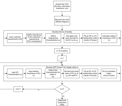
Figure 4-4 shows the process for step 1. First, the voice of the customer is acquired through surveys, focus groups, brainstorm, etc. The information is then organized and structured using techniques such as affinity diagrams. Then, the House of Quality is built: input the customer requirements (based on the voice of customer) on left side of matrix; define and input the importance of the customer requirements; define and input the engineering characteristics xi on top of matrix; set boundaries for the

engineering characteristics; determine the relation between customer requirements and engineering characteristics (center of the matrix); and calculate the relative importance of the engineering characteristics ri. Then, n is defined as the total number of options and

the counter k set to 1 (k=1,2,...,n). Next, the QFD matrix for design option 1 is built: enter engineering characteristics xi on left side of matrix; input the relative importance ri;

determine and input on top of matrix the part characteristics yj for designoption 1; set

best and worst performance levels for all part characteristics (yjb and yjw); determine the

relation between engineering characteristics xi and part characteristics yj (center of

matrix); determine correlation between part characteristics yj (top of matrix, above part

characteristics). Then, if counter k is not equal to total number of alternatives n, add 1 to the counter and repeat the House II process for next design option; otherwise, proceed to next process which is to determine the customer utility.

28 Acquire the VOC

(Surveys, interviews, brainstorm, etc)

Structure the VOC (Affinity Diagram)

k=n?

k=k+1 no

yes

Develop QFD House II for design option k Define Part

Characteristics for option k

(yj)

Set best and worst value of PC (yjb &

yjw) for option k

Fill up EC vs PC relationship matrix (center of house) Input EC

Characteristics (xi)

Input relative importance of EC

(ri)

Fill up correlation matrix (roof of house) k=1

Develop House of Quality Define importance

of the customers requirements (Pair comparison)

Define Engineering Characteristics (xi)

Set upper and lower bounds for the EC (xil & xiu)

Fill up CR vs. EC relationship matrix (center of house)

Calculate relative importance of EC

(ri)

Input customer requirements (CR)

n= # of options

Determine Customer’s

Utility

29 4.2.Design Utility Perceived by the Customer

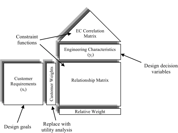
The utility perceived by the customer will increase as the product satisfies the customer needs. To achieve this it would be necessary to find the optimal value of the engineering characteristics the design should have to satisfy the customer requirements. These values could be obtained by using and adapting a design tool that involves multiattribute design optimization proposed by Thurston (Locascio & Thurston, 1993; 1993; 1994). The approach utilizes information from the House of Quality and relates it with multiattribute utility theory. Figure 4-5 shows the interpretation given to the HOQ for the optimization. In the left side of the house, customer requirements are the design goals xi for i=1,2,…3. The engineering characteristics at the top the house represent the

decision variables of the design, which will be yj for j=1,2,…3. The relationship matrix

that links the customer requirements with the engineering characteristics represents the constraint functions. The customer relative importance weight is replaced by the utility function Ui(xi) for each characteristic.

Constraint functions

Relationship Matrix Customer

Requirements (xi)

Cu

st

om

er

W

ei

gh

ts

Engineering Characteristics (yj)

Relative Weight EC Correlation

Matrix

Design goals

Design decision variables

Replace with utility analysis

30

The objective function is the maximization of the design quality, and quality is of the multiplicative form of the multiattribute utility function. This function is originated from classical multiattribute utility theory (von Neuman & Morgenster, 1947; Keeney & Raiffa, 1976). The function contains each single attribute utility function and models the aggregate contribution of all design attributes towards the goal of maximizing the quality.

𝑚𝑎𝑥𝑈 𝑥 𝑦 =_!! ! 𝐾𝑎_!𝑈_! 𝑥_! 𝑦 +1 −1

!!! (4.2)

𝑠𝑢𝑏𝑗𝑒𝑐𝑡  𝑡𝑜      𝑥_! = 𝑔_{! !}      𝑓𝑜𝑟  𝑖=1,2,…,𝑛

𝑦_!" ≤𝑦_! ≤ 𝑦_!"      𝑓𝑜𝑟  𝑗= 1,2,…𝑚

Where 𝑈 𝑥 = overall utility of a design alternative characterized by the vector of

attributes x=(x1,…, xn)

i = 1,2,…, n attributes

j = 1,2,…, m engineering characteristics xi = performance level of attribute i

𝑈! 𝑥! = single attribute utility for attribute i

ai = single attribute scaling constant

gi = constraint function relating attribute i to the design variables

K = normalizing constant, derived from

1+𝐾 = ! 1+𝐾𝑎_!

!!! (4.3)

The single utility functions for each attribute Ui (xi) are obtained by asking

question based on lottery theory (see Appendix I). These functions depict the utility the customer gives to certain engineering characteristic (xi) at different levels of

performance. For this, the designer considers the same product with two different levels of performance of a specific characteristic xi. One level is known with certainty to be

some value x, and the other level is a lottery of p and 1-p of the best and worst performance levels of that characteristic (Figure 4-6). Then, determine the performance

Certain level of Performance

X1

Xbest

Xworst p

1-p

Lottery

or

Certainty

31

level in which the user feels indifferent between the certainty and the probability by responding to the question ‘Which do you prefer, the certainty, the lottery, or are you indifferent?’ If the answer is either the certainty or the lottery, the value of the certainty is changed to a value in between the previous and the last level. Then answers the question again and iterates until the answers is that the user is indifferent between the certainty and the probability. The values derived from answering the lottery questions define the points of the utility functions. Single attribute utility functions are normalized where 𝑈! 𝑥!" =

1 is the highest utility and 𝑈_! 𝑥_!" = 0 is the lowest utility of the attribute.

The scaling constant ai represents the trade-off the designer is willing to make

among the attributes and is determined using similar lottery techniques. The designer is asked again to consider the product with two different configurations of part characteristics. One configuration is a certainty that the characteristic xi is in its best

performance level, and the rest of the attributes are in worst level (x1l,…, xiu,…, xnl). The

other configuration is a probability p that all the characteristics are in their best level

(x1u,…, xiu,…, xnu) and 1-p of all characteristics in worst performance level(x1l,…, xil,…,

xnl). The constant ai is the probability p to which the user feels indifferent between the

certainty and the lottery.

Constraints xi=gi(y) are extracted from the relationship and correlation matrixes in

house II. In order to simplify the use of constraints in the model, scaled engineering and part characteristics are used rather than absolute values, to capture the influence of the parts on the engineering characteristics. Relative engineering characteristics xi’, in terms

of scaled engineering characteristics yi’, are defined. Relative constraints are given by

xi’=gi’ (y). The allowable range for scaled part characteristics yi’ are 0 to 1; and for

engineering characteristics xi’ are the minimum and maximum values of each constraint

xi’=gi’ (y), subject to limits in y’ [0,1]. The actual ranges of engineering and part

characteristics are known from the development of the house of quality and houses II, so any value of xi’ or yi’ can be mapped to the original unscaled values using a simple

32

Thurston’s approach applies multiattribute utility theory to the House of Quality (house I of QFD) to translate, in a mathematical form, the customer’s requirements into engineering characteristics. However, in order to allow the execution of further steps in the proposed framework, the multiattribute utility theory will be applied in the house II. In that case the same interpretation given to the HOQ will be given to the house II but using engineering characteristics instead of customer requirements and part characteristics instead of engineering characteristic.

The outcome of this process would be the value of customer’s utility for each design option and the corresponding vectors of optimal engineering characteristics.

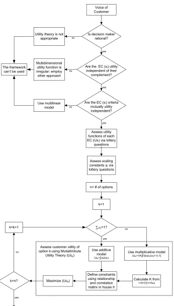
Figure 4-7 shows the process for step 2. This process is an adaptation of the procedure shown by Beroggi (1999). Prior to the calculation of the Customer’s utility three assumptions needs to be confirmed in order to use the multiattribute utility analysis: first, the decision maker must be rational; second, the engineering characteristics xi

should be utility independent of their compliment; and third, the engineering characteristics xi should be mutually utility independent. If any of these conditions are not

met, multiattribute utility function may not be used and, the framework may become ineffective. Otherwise, proceed to assess the utility function of each engineering characteristics Uxi via lottery questions. Then, assess the scaling constant ai also

employing lottery questions. Again n is defined as the total number of design alternatives and the counter k reset to 1 (k=1,2,...,n). If the sum of all scaling constants is 1, the multiattribute additive model Uck=ΣaiU(xi) may be employed (not considered in the

proposed framework); otherwise, employ multiplicative model Uck=1/K[ΠkaiU(xi)+1]-1

for design option 1. K is calculated from the equation 1+K=Π(1+Kai). Next, constraints

are defined from the from the relationship and correlation matrices in the house II of

design option 1. Next, maximize the objective function Uck to obtain the customer utility

33 Figure 4-7 Detailed framework for step 2: Customer Utility

k=n?

no

yes

k=k+1 ∑iai=1?

Use additive model

Uck=∑aiU(xi)

Use multiplicative model

Uck=1/K[∏(kaiUi(xi)+1)-1]

Maximize (Uck)

yes no Customer’s Utility Define constraints using relationship and correlation matrix in house II Is decision maker

rational?

Are the EC (xi) utility

independent of their complement?

Are the EC (xi) criteria

mutually utility independent? Utility theory is not

appropriate

Multidimensional utility function is irregular: employ other approach

Assess utility functions of each EC (Uxi) via lottery

questions

Assess scaling constants ai via lottery questions Use multilinear model yes yes no no no yes Estimate Producer’s Utility Voice of Customer k=1 n= # of options The framework

can’t be used

Calculate K from

1+K=∏(1+Kai)

Assess customer utility of option kusing Mutiattrirbute

34 4.3.Design Utility Perceived by the Producer

The design utility for the producer should reflect the degree in which customers acquire the product. Among other factors, this is a function of the utility of the product design as perceived by the customer. The underlying idea in this section is to estimate the probability that a design alternative is acquired by the customers based on the utility of such an alternative as perceived by the customer.

This is accomplished by adapting the discrete choice analysis method Logit to estimate consumer demand (Train, 2002). It assumes that the customer buy based on the utility value of each product alternative. It also assumes that “as one product’s market share increases, the shares of all competitors are reduced in equal proportion” (Skerlos, Morrow, & Michalek, 2005). This property is called independence from irrelevant alternatives (IIA). In this framework, the model will used to estimate the utility of design alternatives to the Producers.

Let Uck be the utility of option k perceived by customer. Assuming rationality, the

customer will acquire option k rather than option l if and only if the utility of k is higher that the utility of l, that is,  Uc_!  >Uc_!      ∀  k ≠l. This utility, well known by the consumer, is not fully known by the designer, since the designer only perceives the attributes xi of the products chosen by the customer, and perhaps only a few customers’ attributes (s). These two attributes compose a utility function that can relate the observed factors to the

customer’s utility. The function is denoted Vk = V(xi, s) ∀𝑖 , and called “representative

utility”. Since there are utility attributes of which the designer are not aware of then, Vk ≠

Uck. These unknown factors are denoted εk and are defined as the difference between the

true customer utility and the customer utility as captured by the designer. Hence, the true customer utility would be Uck = Vnk + εnk. The designer does not know the value of εnk, so it is here modeled as a stochastic error component. Therefore, the probability that option k be acquired over option l by the customer is:

35

The Logit model assumes that the component ε of the utility U is identically independent distributed (iid) for each alternative and follows an extreme value or double exponential distribution. Then, the probability that the customer acquire the product k will be

𝑃_! =   !!_!!!_!

! (4.4)

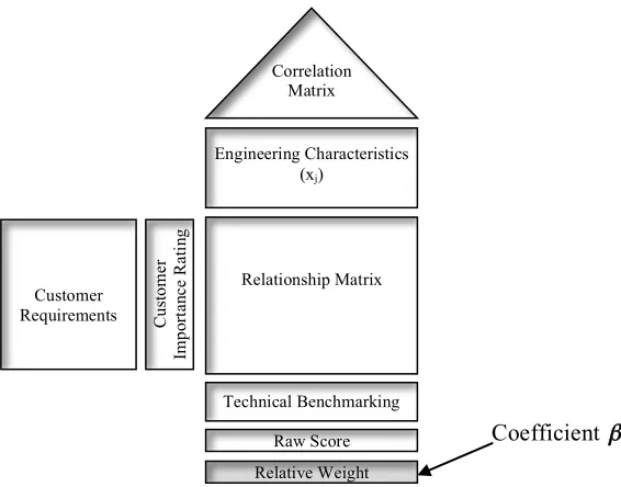
where K is the total number of available alternatives. The representative utility usually is considered in parameters Vk = β’xk, where xk is a vector of observed attributes of option k and β is a corresponding vector of coefficients of the observed attributes which represents the importance that the customer gives to each attribute. The vector β links the producer’s utility to the customer preferences. So, the probability can be written as follow:

𝑃_! =   !𝜷_!’𝒙𝜷𝒌’𝒙_𝒌

! (4.5)

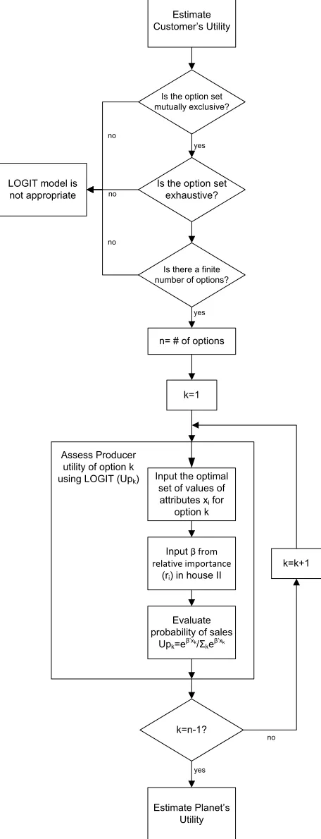
36

Figure 4-9 shows the detailed process for step 3. For this step, 3 more assumptions need to be confirmed: the design options are mutually exclusive, meaning that if one option is selected, the other options are not; the option set must be exhaustive, meaning that the decision maker must choose one alternative; and the number of options must be finite. If any of these conditions are not met, the LOGIT model can not be employed, therefore the framework is can not be used either; otherwise, once again n is defined as the total number of design alternatives and the counter k reset to 1 (k=1,2,...,n). Then, proceed to assess the Producer’s utility of option 1 by entering the set of values of attribute xi and the set of relative importance ri into the equation Upk=eβxk/Σkeβxk. Then, if

counter k is not equal to total number of alternatives n, add 1 to the counter and repeat the Producer’s utility assessment process for the next design option; otherwise, proceed to estimate the Planet’s utility.

Coefficientβ

Relationship Matrix Customer

Requirements _Cust

om

er

Im

po

rt

an

ce

R

at

in

g

Engineering Characteristics (xj)

Technical Benchmarking

Raw Score

Relative Weight Correlation

Matrix

37 Figure 4-9 Detailed framework for step 3: Producer’s Utility

k=n-1?

k=k+1

no

yes

Estimate Planet’s Utility

Is the option set mutually exclusive?

Is the option set exhaustive?

yes

Is there a finite number of options?

LOGIT model is not appropriate

no

no no

yes

k=1

Producer’s Utility

Evaluate probability of sales

Upk=eβ’xk/Σkeβ’xk

Input the optimal set of values of

attributes xi for

option k

Input β  from   relative  importance  

(ri) in house II

Estimate Customer’s Utility

Assess Producer utility of option k using LOGIT (Upk)

38 4.4.Design Utility Perceived by the Environment

To estimate the environmental impact of the products, life cycle assessment tools are suggested. Typically, these approaches consider impacts on human health, ecosystem quality, and resource depletion. Although preferred, quantitative approaches (such as process-based LCAs Eco-Indicator 99) tend to be more time consuming and rely on a detailed bill of materials which may not be available early on the design stage. Streamlined LCAs are simpler and can be developed with a less defined bill of materials but provide somewhat subjective information. Ultimately, the selection of the environmental assessment approach will depend on the level of product definition that can be achieved.

From the environments’ perspective, producing products with zero or positive environmental impact is the ideal condition. However, almost all products generate a negative impact throughout its respective lifecycles, or at least in some stages of it. Consider the lifecycle of synthetic carpet. Negative environmental impacts that accrue along the lifecycle of this product include the harvesting of a non renewable material (natural gas and petroleum) as the feedstock, emissions associated with the generation of the power used during the manufacturing stage, emissions associated with the transportation of the product from the producer to the consumer, outgassing of potentially hazardous vapors during the use stage, and the eventual disposal of the material in a landfill. Many products, be they appliances, automobiles, or building materials exhibit similar impact patterns.

Here, a design option is considered to have high utility to the environment if its impact is minimal. In other words, the utility to the environment increases as the product’s environmental impact decreases.

The design utility to the environment will be described by the following proposed function:

39

where:

Ue : utility of the design perceived by the environment,

I: an impact factor that is a function of the nature of the product

X: the impact assessment of the design (obtained from LCA tools).

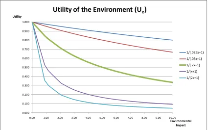
The function depicts a family of curves some of which shown in Figure 4-10 where the environmental impact (units in eco-points or equivalent) is drawn with respect to the environments’s utility of the design.

Ideally the highest utility to the Planet will be reached either having a product with no environmental impact, or by not manufacturing any product, which is not considered as a possible option in the framework; therefore, a design with no environmental impact will generate the highest utility to the Planet. This ideal case would have utility value of 1. The steep initial decline depicts the impact associated with the mere existence of the product. A large portion of this can be thought of “fixed impacts”, a

0.000 0.100 0.200 0.300 0.400 0.500 0.600 0.700 0.800 0.900 1.000

0.00 1.00 2.00 3.00 4.00 5.00 6.00 7.00 8.00 9.00 10.00

1/(.025x+1) 1/(.05x+1) 1/(.2x+1) 1/(x+1) 1/(2x+1)

Utility  of  the  Environment  (U

)

Utility

Environmental   Impact

40

consequence of the fact that a new product, regardless of how environmentally friendly it happens to be, would always require some amount of raw materials, energy, etc. This changes the status quo in a significant way, which is reflected in this function.

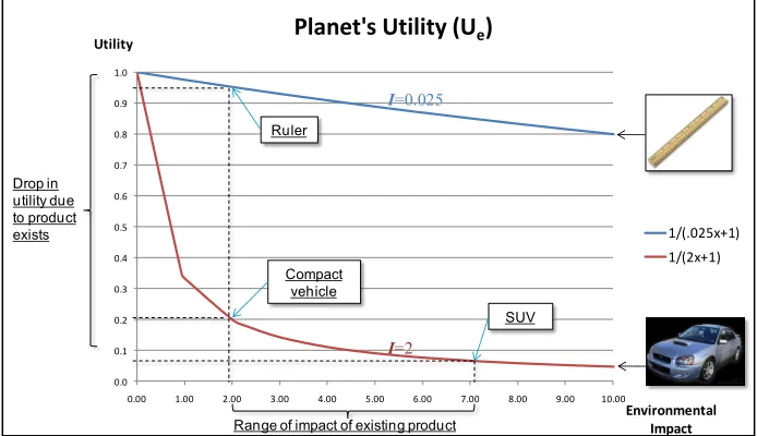
For example, consider two types of vehicles, compact and SUV. Assume that they are fabricated using similar materials. Compact vehicles pose smaller mass, and are equipped with smaller engines that typically consume less gas than SUVs; therefore, they may cause less environmental impact and generate higher utility to the Planet (Figure 4-11). But, even if the compact vehicle is improved to reduce the impact (e.g. Hybrid technology, use of recycled materials, etc) there always exists a minimum impact associated with the creation of the product. The asymptotic shape of the curve implies a diminishing rate of impact with marginal increases of environmental impact. Different design choices, technological advances, etc. will position the design along different points in the curve.

Now consider two different types of products, a wooden ruler and a vehicle. The ruler and the vehicle will have different environmental impacts. The quantity of material and processes required to fabricate one finished wooden ruler is significantly smaller than the quantity required for one vehicle; additionally, the logistics involved in the transportation of materials and final products is much smaller for the wooden ruler than

0.0 0.1 0.2 0.3 0.4 0.5 0.6 0.7 0.8 0.9 1.0

0.00 1.00 2.00 3.00 4.00 5.00 6.00 7.00 8.00 9.00 10.00

1/(.025x+1) 1/(2x+1)

Planet's Utility  (Ue)

Utility

Environmental   Impact

Drop in utility due to product exists

Range of impact of existing product Compact

vehicle

SUV Ruler

Figure 4-11 Scaling of the utility function of the planet. I=0.025

41

for the vehicle. Therefore, can be implied that the environmental impact of a ruler is much smaller than the generated by the vehicle. Compared to the vehicle, the initial “fixed impacts” of the wooden ruler are minor; hence the utility of the vehicle drops faster as both products are created (also Figure 4-11). Thus, the impact factor I is used to scale the utility curves depending on the nature of the products. It is assigned by the designer based on his/her criteria about the products nature. In general, more complex and bigger products may generate more environmental impacts compared to simpler and small ones, so the factor I is greater.

For the proposed framework, Eco-Indicator 99 will be employed to estimate the environmental impact of the products. Although it is a time consuming process, it becomes very useful due to the outcome which is a value called Ecoindicator. This single and simple indicator can then be easily incorporated into the framework to calculate the design utility perceived by the environment using the equation 6.

Figure 4-12 shows the process of step 4. After the producer’s utility is estimated, the bill of materials for each of the design alternative is created. Then, the designer based

on the products nature sets the value of impact factor I. Once again n is defined as the

42 Figure 4-12 Detailed framework for step 4: Planet’s Utility

k=1

k=n?

k=k+1 _no

Calculate Global Utility

yes

Planet’s Utility

LCA Input Bill of Material

and weights Estimate Producer’s Utility

Assess Planet utility of option k using either

streamline LCA or ecoindicator 99 depending on level of

detail (Uek)

n= # of options

Calculate Planet’s utility

Ue=1/(IX+1)

Develop bill of material for each design option

Define value of impact

43 4.5.Global Utility

Lastly, the Global Utility will be defined by the sum of the products of the utility to the customer, the producer, and the planet by the respective weight coefficient

(4.7)

where :

UGk: Global Utility of design option k.

a: weight factor vector (cardinality = 3)

a = [ac,ap,ae]

ac+ap+ae=1 (4.8)

Uc = Design utility perceived by customer

Up = Design utility perceived by producer

Ue = Design utility perceived by the environment.

The global utility must be scale between 0 and 1. Therefore, the sum of coefficients ac, ap, and ae add up to 1. These coefficients reflect the importance each

utility have respect to each other. Manipulating these factors, different design tendencies can be described. For example, a neutral global utility is that one that gives equal importance to each of the stakeholders, so no preference is defined. But, a designer with environmental consciousness that strives to reduce the impact to the environment will

assign higher importance to the planet increasing ae and diminish the importance to one

or both the customer and the producer utilities ac and ap respectively. On the other hand,

an environmentally oblivious designer that is focused on the benefits to the producer and customer will increase one or both the customer and/or producer’s utility ac and ap at

expenses of the environment impact reducing the importance of the utility to the planet ae.

e e p p c c k

G a U a U aU

44

Generally the customer drives the products success by using the purchase power to buy or not the product and thus rewards the producer. Therefore, designers ideally will

not diminish the importance of the utility to the customer ac below the importance of the

producer and planet.

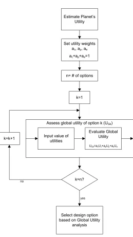
The process for the calculation of global utility is shown in Figure 4-13. Once the utility for the Planet is calculated, individual utility weights ac, ap, and ae are set

according to the design tendency (customer, producer, or environmentally focused). The sum of the utility weights should be equal to 1. Again, n is defined as the total number of design alternatives and the counter k reset to 1 (k=1,2,...,n). Then, the Global utility for option 1 is calculated by entering the utility values Uc, Up, and Ue, and the respective

utility weights ac, ap, and ae in the equation UGk= ac Uc+ap Up+aeUe. Then, if counter k is

45 Figure 4-13 Detailed framework for step 5: Global Utility

k=n? k=k+1

no

Select design option based on Global Utility

analysis

yes

k=1

Global Utility

Estimate Planet’s Utility

Assess global utility of option k (UGk)

Set utility weights ac, ap, ae

ac+ap+ae=1

Input value of utilities

Evaluate Global Utility

UGk=acUc+apUp+aeUe

46

5.

Case Study

The following is a hypothetical case involving real products to illustrate how the framework can be used.

According to the Energy Information Administration, in 2009 U.S. homes consumed approximately 15.3% of the energy in lighting (indoor and outdoor) (US Energy Information Admninistration, 2009). Illuminating outdoor spaces, safety and security, beauty, and home best usage are some of the benefits of having illuminated home outdoors.

A producer of light devices has identified in this area a business opportunity. So, it was decided to research and design a product that satisfy these customers’ needs while increasing market share and being environmentally responsible. The producer also decided to investigate existing alternatives implementing the proposed framework. Using the framework, the producer will be able to benchmark these existing products estimating their global utility, and predict the impact of design changes during design iterations.

5.1.Voice of the Customer and Quality Function Deployment

47

price (letter A in the

Table 5-1 Scale Pair Comparison

matrix) than the longevit