Pseudo-Zernike based multi-pass automatic target recognition from multi-channel SAR

Published in IET Radar, Sonar and Navigation Received on 16th April 2014

Revised on 29th July 2014 Accepted on 3rd August 2014 doi: 10.1049/iet-rsn.2014.0296

ISSN 1751-8784

Pseudo-Zernike-based multi-pass automatic target

recognition from multi-channel synthetic

aperture radar

Carmine Clemente

_{, Luca Pallotta}

_{, Ian Proudler}

_{, Antonio De Maio}

_{, John J. Soraghan}

_,

Alfonso Farina

1

Department of Electronic and Electrical Engineering, University of Strathclyde, CeSIP, 204 George Street, G1 1XW, Glasgow, UK

2

CNIT, viale G.P. Usberti, n. 181/A–43124 Parma, c/o udr Università‘Federico II’, via Claudio 21, I-80125 Napoli, Italy 3_{School of Electronic, Electrical and Systems Engineering, Loughborough University, Leicestershire, UK}

4

DIETI, Università di Napoli‘Federico II’, via Claudio 21, I-80125 Napoli, Italy 5_{Selex ES, via Tiburtina Km.12.4, I-00131 Roma, Italy}

E-mail: [email protected]

Abstract: The capability to exploit multiple sources of information is of fundamental importance in a battlefield scenario. Information obtained from different sources, and separated in space and time, provides the opportunity to exploit diversities to mitigate uncertainty. In this study, the authors address the problem of automatic target recognition (ATR) from synthetic aperture radar platforms. The author’s approach exploits both channel (e.g. polarisation) and spatial diversity to obtain suitable information for such a critical task. In particular they use the pseudo-Zernike moments (pZm) to extract features representing commercial vehicles to perform target identification. The proposed approach exploits diversities and invariant properties of pZm leading to high confidence ATR, with limited computational complexity and data transfer requirements. The effectiveness of the proposed method is demonstrated using real data from the Gotcha dataset, in different operational configurations and data source availability.

1 Introduction

In the modern battlefield scenarios, the availability of multiple sources of information, such as spatial, temporal or other diversities, allows improvements in sensor performance and capabilities. Modern radars scenarios normally involve different diversities. Some of these are provided by the sensor position in the space–time plane. In particular, spatial diversity can be given by multiple platforms observing from different positions, whereas temporal diversity can be provided by multiple passes over the same area from the same platform. Additional diversities are provided by sensor characteristics such as frequency, waveform and polarisation.

In our work, we investigate the possibility of exploiting the combination of the above mentioned categories of diversities. Of particular interest is the ability to achieve high performance results with low cost algorithms and the capability to summarise the discriminating information thereby reducing the communication overhead between sensors.

A particular application of interest for this scenario is automatic target recognition (ATR) [1–3] and its lower level tasks (identification, characterisation and fingerprinting). The challenge of ATR has been investigated from

polarimetric synthetic aperture radar (SAR), inverse SAR (ISAR) and passive bistatic radar [4–8]. The use of polarimetric data is justified by the fact that the way in which targets scatter signals with different polarisations contains information that can be exploited in target recognition, so the use of multi-polarisation SAR data can lead to improved ATR performance. In [4], a combination of polarimetric and frequency dependent features was exploited to distinguish among different targets in a SAR image. The approach represents the electromagnetic scattering with primitive geometries (such as cylinders, spheres, edges, top hats etc.) and the physical geometry of the target, which can be seen as a combination of different elementary geometries. Another approach has been investigated in [5], where a two-dimensional cepstrum-based feature is extracted with the aim of discriminating between clutter and man-made objects in a SAR image. Tests on the MSTAR database have shown good classification results using this technique. A more general approach has been investigated in [9], where L2

classification of stationary ground targets using high resolution, fully polarimetric SAR images. In [6, 10], a comparison of ATR performance for several polarisation/ resolution combinations has been provided (in particular, the single HH polarisation is compared to the optimal combination ofHH,HVandVVpolarisations). The problem of ATR exploiting polarimetric information has been investigated also from ISAR in [7], where persistent polarimetric signatures are exploited, whereas in [8], the problem of ATR has been investigated in passive bistatic radar.

In this paper, a novel algorithm for ATR, with target identification capabilities, from multiple spatially separated, multi-channel SAR data, is presented. The algorithm is capable of exploiting single or multi-channel information. With low-computational cost it extracts reliable and easy-to-share discriminating features based on the pseudo-Zernike moments (pZm) [11]. pZm belong to the family of geometric moments such as Hu and Zernike moments [12, 13], which were used both in image processing for pattern recognition and image reconstruction [14–16]. Some of the main advantages of these moments include position, scale and rotational invariance. Another important property is that pseudo-Zernike are independent moments, because they are computed from orthogonal polynomials. Moreover, pZm have a lower sensitivity to noise than Zernike moments [11] as well as more moments for a given polynomial order. This last property is important as the availability of more independent moments provides more information (to be used for image reconstruction or classification purposes), with lower sensitivity to noise. SAR images are different from ‘everyday’ images. They present peculiar characteristics such as speckle noise, for this reason we select the pZm, for their capability to represent the images with a lower sensitivity to noise than Zernike ones. Although the proposed framework applies to the general multi-channel SAR case, without loss of generality, our experimental analysis will focus on the case of multi-polarimetric SAR. The proposed algorithm is tested with the Gotcha dataset [17] that contains multiple observations of commercial vehicles. The results show that the proposed algorithm provides good classification performance increasing with the use of spatial and polarisation diversity.

This paper is organised as follows. In Section 2, the novel algorithm to extract the features from a multi-channel SAR observation is introduced together with two decision fusion frameworks for the case of multiple passes. Section 3 describes the analysed scenarios and presents the obtained numerical results from real data. Finally, in Section 4, some conclusions and possible future research directions are provided.

2 Classification algorithm based on pZm

In this section, a novel algorithm for automatic target classification in SAR images is presented. Specifically, a new data representation is utilised for both single and multi-channel ATR from SAR. The approach is based on the use pZm [11], in order to obtain reliable feature vectors with relatively small dimension and low computational complexity. Noted that in [18], we have introduced the use of the pZm for ATR applied to micro-Doppler signatures. This novel approach benefits from specific properties of the pZm such as invariance with respect to translation and

rotation, in addition scale invariance can be included if required by the specific application [11].

In the following subsections, the background theory defining the pZm is introduced. Then, the novel feature extraction algorithm and the decision fusion frameworks are presented in detail.

2.1 Pseudo-Zernike moments

Letf(x,y) be a non-negative real image. The complex pZm [11] can be computed as

cn,l=

n+1

p

2p

0 1

0

W_n∗_,l(rcosu,rsinu,r)f(rcosu,rsinu)rdrdu

(1)

where the symbol (·)* indicates the complex conjugate operator andWn,l are the pseudo-Zernike polynomials. The

latter are a set of orthogonal functions that can be written in the form

W_n,l(x,y,r)=W_n,l(rcosu,rsinu,r)=S_n,l(r) eilu (2)

with i=√−1, x=ρcosθ, y=ρsinθ, l is an integer and Sn,l(ρ) is a polynomial (called a radial polynomial) in ρ of

degree n such thatn≥|l|. Notice that the modulus of (2) is rotationally invariant [11]. Moreover, these functions form a complete basis and satisfy, on the unit disc (i.e. for x2+ y2≤1), the orthogonality relation [11]

x2_+y2_≤1

W_n∗_,lx,y,x2+_y2_W

m,k x,y,

x2+_y2

dxdy

= p

n+1dmndkl

(3)

where δmnis the Kronecker delta function, that is, δmn= 1 if

m=n, and 0 otherwise. As given in [11], an explicit expression to compute the radial polynomials, Sn,l(ρ), is

S_n,l(r)=

n−|l|

k=0

rn−k(−1)k(2n+1−k)!

k!(n+ |l| +1−k)!(n− |l| −k)! (4)

Moreover, as previously stated an important characteristic of the pZm is the simple rotational transformation property because of (2); indeed, the moment requires only a phase factor for the rotation [11].

2.2 Feature extraction algorithm

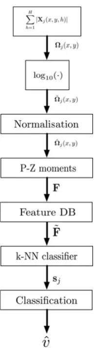
The feature extraction algorithm is summarised in the block diagram shown in Fig. 1, while a detailed explanation of the processing steps are given below.

The complex valued image for each channel from the jth sensor is defined as Xj(x,y,h)[CB×Z×H with x and y

then {HH} is the considered polarisation, while forH= 4 the set of polarisations is {HH,VV,HV,VH}).

The feature extraction algorithm begins with the generation of the multi-channel magnitude image of the target area

Vj(x,y)=

H

h=1

|Xj(x,y,h)| (5)

The aim of this paper is to demonstrate the utility of the proposed framework and of the pZm not to choose the best channel fusion algorithm. The focus is not on the multi-channel fusion technique, thus the simplest fusion technique (5) is utilised. In addition this will result in a lower computational burden of the entire ATR algorithm. However, other fusion approaches exist in literature, particularly for the polarimetric case [10, 19] and can be applied in place of (5).

AsΩj(x,y) can have a very large dynamic range (this can

affect the performance of the algorithm by reducing the sensitivity of the pseudo-Zernike polynomial to targets characteristics), its logarithm is used instead

˜

Vj(x,y)=log10(Vj(x,y)) (6)

To obtain features that are independent of different intensity levels, because of different observation angles and channel propagation properties, a normalisation ofV˜j is required to

restrict its magnitude to the interval [0,1]

Vj(x,y)=V˜j(x,y)−min[V˜j(x,y)]

ˆ

Vj(x,y)=Vj(x,y)/max(Vj(x,y))

This step removes information about the absolute value of the radar cross-section (RCS) of the target. This piece of information can be considered separately in a RCS-based algorithm. Then the outputs of the two algorithms can be used in conjunction to increase the overall performance.

The next step of the algorithm (Fig.1) is the projection of ˆ

Vj(x,y) onto a basis of pseudo-Zernike polynomials. The

polynomials can be pre-computed through (4) since it depends on the sub-image size B×Z only (because of the dependencies of (4) only on ρ), and therefore may be used to populate a look-up table. As the pseudo-Zernike polynomials are defined on the unit disc, the support of the imageVˆ_j(x,y) is scaled, before the moments are computed, to avoid information loss by removing the part of the image under test that resides outside of the unit circle. Applying (1) to Vˆ_j(x,y), the pseudo-Zernike expansion is obtained as

cn,l=

n+1

p

2p

0 1

0

Wn∗,l(rcosu,rsinu,r)Vˆj(rcosu,rsinu)rdrdu

(7)

The output of this stage is the set of (n+ 1)2magnitudes of the pseudo-Zernike coefficients |cn,l|, 1≤l≤(n+ 1)2. From (4),

the modulus of the pZm is rotationally invariant. This means that at a given observation angle the modulus of the moments are independent of the relative orientation of the target in the image plane. For example, a target observed from the same aspect angle in two different images and appearing with a different orientation in the image plane, because of unregistered images, will be represented by the same moments (neglecting the effect of the noise and of the observed scene). Hence, the feature vector is

F= |c0,0|, . . .,|cN,−N|

(8)

Finally, the feature vector, F, is normalised using the following linear rescaling

˜

F=(F−mF)/sF (9)

whereμFandσF are the mean and standard deviation of the

feature vector. These values are then used to populate the Feature Database that is used as input to a classifier.

2.3 Classification and fusion

The last step of the algorithm consists of the classification procedure. The classification has been performed using a k-nearest neighbour (k-NN) classifier because of its low computational load and its capability of providing score values as an output [20, 21]. Other classifiers with similar characteristics could also be selected.

The sum method is selected as fusion rule [20,21]. Two strategies are considered for the fusion, maximum vote and maximum confidence. Let V be the number of possible classes. For each of the J sensors, the k-NN classifier

returns as output a V-dimensional vector sj containing the

confidence levels for each cluster (or the value of the vote [0,1] in case of the rule at maximum vote). The confidence levels (referred also as scores) are defined as the number of nearest neighbours belonging to the vth class divided by k. The vote is defined as 1, if the observation is considered to belong to one of theVclasses, and 0 otherwise. The sum of all the scores or votes is then computed as

l=J j=1

sj (10)

with l = [l1, l2, …, lV]. This fusion strategy allows the

exploitation of the information from multiple images and is known for its robustness [20,21]. In addition, it allows the definition of the ‘unknown’class if a draw occurs, when l does not have a unique maximum element, or if the maximum value of l does not satisfy a specific requirement, such as a sufficient score or vote. In particular, we define a threshold [The threshold value depends on the desired algorithm performance. The selection of the optimal threshold is left to the algorithm user in accordance with the application requirements.] η(i.e. the minimum score or vote to be reached to permit a classification) and all observations with l below η will be not classified and labelled as unknown. Thus the estimated class can be selected as

ˆ

v= arg maxv l

if ∃!(maxl).h

unknown otherwise

(11)

Defining the unknown class is important as the number of unknowns provides a measure of the capability of the ATR system to decide for a class.

3 Performance analysis

In this section, the performance analysis of the ATR algorithm described in Section 2 is presented. The algorithm is applied to real polarimetric X-band SAR data. We first introduce the analysed scenario then we present numerical results obtained on the real data.

3.1 Analysed scenarios

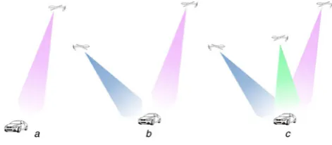
The dataset used in this analysis is the ‘Gotcha Volumetric SAR Data Set V1.0’[17], consisting of SAR phase history from a sensor with carrier frequency of 9.6 GHz and 640 MHz bandwidth, full azimuth coverage, eight different elevation angles and full polarisation. The imaged scene consists of numerous civilian vehicles and calibration targets. For our analysis, the aperture has been divided in sub apertures of 4° in azimuth, leading to approximately equal range-azimuth resolution cells of 23 cm. In this way, 90 images (looks) for each of the 8 circular passes (different elevations) are available in four polarisations, {HH,VV,HV,VH}, for each of the 9 commercial vehicles considered. To allow the reader to understand the imaged targets and scene, in Fig.2the 360° full polarimetric image (obtained adding together the intensities of the four images) of the scene of interest is shown. The image is a multi-look image (adding all the 90 looks of one circular pass). As already mentioned, for testing purposes a single look is used. In Fig. 2, the nine vehicles are labelled with

alphabetic letters. Specifically, the nine vehicles are, respectively, (A) Chevrolet Prizm, (B) Nissan Sentra, (C) Nissan Maxima, (D) CASE Tractor, (E) Ford Taurus, (F) Chevrolet Camry, (G) Hyundai Santa Fe, (H) Chevrolet Malibu and (I) Hyster Forklift.

To perform the analysis equal sized sub-images (50 × 50 pixels) containing each vehicle have been selected. Specifically, of the eight available passes (different elevations) a subset of the pass with lowest altitude is used to train the classifier while all the other images (i.e. the unused images from the lowest pass and all the images from the other seven, higher elevation, passes) are used to test the algorithm. In this way, different elevation and azimuth angles are considered for testing the images to provide independent training and validation sets.

The analyses have been conducted considering different choices of the training subset, specifically three training sets composed of images selected with azimuth spacing of 12°, 30° and 92°, respectively. The use of a limited number of aspect angles for training is meaningful in terms of a practical realisation. Specifically, the acquisition of a database covering all the possible different aspect angles is expensive, time demanding and in some cases impossible. Thus having an under-sampled database of training observation is a valid test for the proposed algorithm. The analysis is performed using 1, 2 and 3 randomly selected test data images to characterise the benefits of the multi-sensor framework and the classification fusion stages. Moreover, a comparison between the fusion techniques exploiting the output scores and votes of the k-NN

Fig. 3 1, 2 and 3 sensors acquisition examples a1 Platform

b2 Platforms c3 Platforms

classifier, respectively, have been considered. The analysis has been also conducted considering a single polarisation (SP) and full polarisation (FP) analysis. To evaluate the performance of the classification algorithm, the correct classification in percentage, defined as the number of correctly classified sub-images over the total number of sub-images under test, is used as figure of merit. For the case of 1 test image all the available images have been used, whereas for the case of 2 and 3 test images 10 000 pairs or triples are chosen randomly. For this reason, the standard deviation of the correct classification rate for the cases of 2 and 3 sensors is also computed.

In Fig. 3, examples of the configurations considered are shown. Multiple acquisitions can be assumed to be done by multiple platforms or from the same platform in different instants of time. Moreover, the analysis is performed for different ordersnof the pZm between 1 and 20 and using a k-NN classifier, analysing different values of k. The range of values ofnis selected considering that the sensitivity to noise increases with n, thus making it less useful to use moments of higher order.

3.2 Numerical results

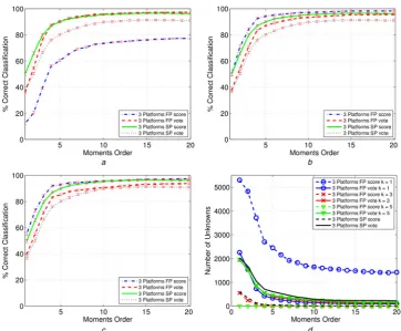
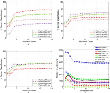
Thefirst analysis is presented in Fig.4showing the results obtained for 3 platforms using a training samples spacing of 12°, equivalent to 30 observations of a target with different cases of equally spaced initial azimuth angles (e.g. 0°, 12°,

24° etc.). The curves refer to both SP and FP cases, and both the classifier based on the score and vote fusion rules have been analysed. Moreover, the subplots (a)–(c) of Fig. 4 refer to three different values of the parameter k in the k-NN classifier, that is, k= 1, 3, 5. Finally, in subplot (d) of Fig. 4the number of unknowns obtained in the above cases are given against the moment orders. Moreover, the 3σ confidence intervals are quite small (less than 1−2%). The curves show that in general, the FP case produces a higher level of correct classification with respect to the SP one, for the same k and score/vote choice. However, this behaviour is not observed in the first case, k= 1, for the fusion rule based on the score. The curves also show that the correct classification increases as the moment order increases. However, as suggested previously the simulation results shown in Fig. 4 show a saturation in performance with increasing moment order. The higher order of moments are increasingly influenced by the noise. Consequently they do not introduce additional discriminating information. As expected the number of unknowns reduces as the moment order increases, and the curves reflect the same behaviour observed for subplots (a)– (c). Finally, it is important to underline that the maximum correct classification is obtained in the FP case with k= 3 and with the use of the score-based rule.

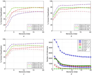
Fig. 5shows the results obtained for 3 platforms using a training samples spacing of 36°, equivalent to 10 observations of a target with different initial azimuth angles

Fig. 4 Correct classification (%) against moments order of the proposed algorithm for training samples spaced 12° with 3 platforms Both FP and SP cases have been considered with score and vote-based fusion rules

Threshold is set to 1 and 2 for the score and vote rules, respectively Subplots (a)–(c) refer tok= 1, 3, 5 for the k-NN classifier

In subplot (d), the number of unknowns is given against the moments order a k= 1

b k= 3 c k= 5

and equal azimuth spacing. Again, the curves refer to both SP and FP cases. Both the classifier based on the score and vote fusion rules have been analysed. Also for this analysis, three different values of the parameterkin the k-NN classifier, that is,k= 1, 3, 5, have been considered [see subplots (a)–(c) of Fig. 5], whereas Fig. 5d shows the number of unknowns against the moment orders. Also in this second case, the 3σ confidence intervals are quite small (less than 1−2%). The analysis conducted here is in agreement with the results obtained in the previous case, namely the FP system can reach a higher level of correct classification with respect to the SP one. Moreover, the classifier based on the score fusion rule outperforms that based on the vote fusion rule. However, comparing the curves of Fig. 5 with those of Fig. 4, it can be observed that increasing the azimuth spacing between the images causes the performance of the classifier to decrease because of the reduced number of training images. Also, in this case, the number of ‘unknown’ classifications still reflects the behaviour observed for subplots (a)–(c). Finally, it is important to underline that the maximum correct classification is obtained in the FP case with k= 3 and with the use of the score-based rule.

The results obtained for the case considering 3 platforms and training samples spacing of 92°, equivalent to 4 observations of a target with different initial azimuth angles and equal azimuth spacing, are shown in Fig.6. Again, the curves refer to both SP and FP cases as for the previously

analysed scenarios. As observed for the first two situations, also for this case the 3σconfidence intervals are quite small (more or less 1−2%). Again, the FP system produces a higher level of correct classification with respect to the SP one. The classifier based on the score fusion rule still outperforms the one based on the vote fusion rule, and a performance degradation with respect to the previously analysed cases is observed. Also the number of unknowns is greater than those obtained in the other cases. To conclude this analysis, it can be claimed that the value k= 3 with the FP system produces the best classification performances between the considered situations. In addition the score fusion rule outperforms the vote one.

In Fig.7, the correct classification expressed in percentage is given against the moment orders for the classifiers based on the pZm, for the case of 12° of spacing between training samples in azimuth. For comparison purposes the L2

norm-based algorithm has also been considered [9]. More precisely, the L2 norm-based algorithm extracts the

sub-image containing the object to classify and normalises it in order to ensure unit norm. Then, this normalised image is given as input to the classifier. This algorithm was selected as benchmark as it considers all the information available in the image to perform the classification. Moreover, Fig. 7compares the results obtained considering observations from 1, 2 or 3 platforms, with a 3-NN classifier. As the vote rule was outperformed by the score decision rule in the previous analysis for k= 3, in this

Fig. 5 Correct classification (%) against moments order of the proposed algorithm for training samples spaced 36° with 3 platforms Both FP and SP cases have been considered with score and vote-based fusion rules

Threshold is set to 1 and 2 for the score and vote rules, respectively Subplots (a)–(c) refer tok= 1, 3, 5 for the k-NN classifier

In subplot (d), the number of unknowns is given against the moments order a k= 1

b k= 3 c k= 5

analysis we consider for conciseness only the latter. The number of unknowns is reported in Fig.7subplot (b). Note that the results shown in Fig. 7are obtained considering a higher threshold with respect to those of Figs. 4–6. This selection is motivated by the need to provide results showing the effectiveness of the algorithm with a different

threshold set-up. It was the last parameter to vary in order to complete the parametric analysis of the presented algorithm. Moreover, a higher threshold can be required in more demanding scenarios. For example a higher threshold might be needed in a scenario where the capability to identify correctly a target with high confidence is a critical

Fig. 6 Correct classification (%) against moments order of the proposed algorithm for training samples spaced 92° with 3 platforms Both FP and SP cases have been considered with score and vote-based fusion rules

Threshold is set to 1 and 2 for the score and vote rules, respectively Subplots (a)–(c) refer tok= 1, 3, 5 for the k-NN classifier

In subplot (d), the number of unknowns is given against the moments order a k= 1

b k= 3 c k= 5

dNumber of unknowns

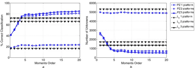
Fig. 7 Correct classification (%) against moments order of the proposed algorithm with pZm and the L2norm-based algorithm, for 12° of spacing in azimuth between training samples, with 1, 2 and 3 platforms

FP case has been considered with score-based fusion rule, subplot (a), whereas the threshold is set to 1 for the case of 1 and 2 sensors and 4/3 for the 3 sensors case Moreover a 3-NN classifier is utilised

In subplot (b), the number of unknowns is given against the moments order aScore

feature (i.e. in the case of engaging a target). In the analysis presented in Fig.7, for the cases of 1 and 2 sensors a score of at least 1 was considered to be able to classify, while the value of 4/3 was the minimum score considered in the case of 3 sensors. The conducted analysis has shown that the algorithm based on pseudo-Zernike and the L2-based

algorithm can achieve comparable performance when pZm of order 10 are considered. However, the former uses aB× Z-dimensional space for the features, while the proposed approach uses a space of (N+ 1)2withN≤20, meaning that our approach for N= 10 on an image of sizes B=Z= 50 requires 121 components of the feature vector while the L2

approach requires 2500 components. This is a significant advantage in terms of computational complexity and bandwidth requirements. Finally, observing both the correct classification and the number of unknowns, it can be seen that the higher the number of platforms, the better the classification results.

The results shown in Fig. 8 refer to the case of 36° of spacing between training samples in azimuth. The results show the correct classification versus the moment orders achieved by the classifiers based on the pZm and on the L2

norm. In Fig. 8, a comparison between the algorithms that exploit different numbers of platforms is provided. Again we consider the score decision rule and a 3-NN classifier. The results obtained in this analysis confirm those shown in Fig. 7. In general, compared with the results in Fig. 7, the performance degradation is obtained if fewer aspect angles are used as training samples. In addition, the L2algorithm

does not perform as well as the pseudo-Zernike based in this case, demonstrating a higher sensitivity to a smaller number of training samples.

Finally, in Fig.9, the correct classification is plotted against the moment orders, for the classifiers based on pZm and on the L2 norm, for the case of 92° of spacing between

training samples in azimuth. Again, the behaviour analysed in Figs. 7 and 8is still evident in this last case. However, because of the large spacing between training samples, the performance degradation increases; all the algorithms are unable to produce a correct classification score higher than 60% and they are also not able to provide a number of unknowns less than 2500. Notice also, that in this last analysis the performance of the L2-based algorithm has

deteriorated more than those of the pseudo-Zernike approach.

Fig. 8 Correct classification (%) against moments order of the proposed algorithm with pZm (open circles–marked blue curves) and the L2 norm-based algorithm, for 36° of spacing in azimuth between training samples, with 1, 2 and 3 platforms

FP case has been considered with score fusion rule, subplots (a), whereas the threshold is set to 1 for the case of 1 and 2 sensors and 4/3 for the 3 sensors case Moreover a 3-NN classifier is utilised

In subplot (b), the number of unknowns is given against the moments order aScore

bNumber of unknowns

Fig. 9 Correct classification (%) against moments order of the proposed algorithm with pZm and the L2norm-based algorithm, for 92° of spacing in azimuth between training samples, with 1, 2 and 3 platforms

FP case has been considered with score fusion rule, subplots (a), whereas the threshold is set to 1 for the case of 1 and 2 sensors and 4/3 for the 3 sensors case Moreover a 3-NN classifier is utilised

In subplot (b), the number of unknowns is given against the moments order aScore

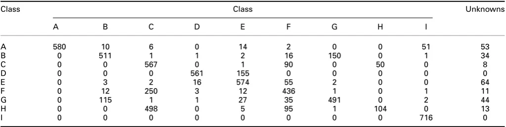
To complete the analysis of the proposed ATR algorithm, in Tables1and 2, two examples of confusion matrices are shown. The analysis is conducted with 3 sensors, with FP and an image spacing of 12° for the results in Table1, and 92° for the results in Table 2, respectively. In both cases, the pZm of order 20 was used,k= 3 and the threshold was 4/3. From the results in the tables, it can be seen how for some targets (i.e. B, D and G) the increased number of aspect angles used for training improves the classification capabilities, while for other targets (i.e. C, E and H) there are still few cases of incorrect classification and unknowns.

In general, the presented analysis demonstrates that the use of the score rule to assign the classes provides better performances together with the use of 3 nearest neighbours in the classifier. Moreover the better capability of the pZm to characterise the targets over the L2-based approach has

been highlighted. Finally, in all the analysed cases the performance improves with the number of aspect angles available and with the number of observations from different aspect angles used to perform the classification.

Clearly, the proposed algorithm appears to have multiple advantages: reliable target identification, multi-observation fusion capabilities without the requirement of a multi-platform training set, ability to provide good automatic target identification performance with a limited set of target observations as training. The pZm properties of translation and rotation independence makes the algorithm robust with respect to the relative target orientation in the image plane and with no requirement for images to be registered between different platforms.

4 Conclusion

In this paper, a novel algorithm for ATR with the capability of target identification has been presented. The proposed algorithm exploits the pZm derived from multi-channel

SAR images as features used to identify different targets. The algorithm allows the fusion of the classification result of each of multiple observations from different aspect angles. A performance analysis using the ‘Gotcha Volumetric SAR Data Set V1.0’ has been performed considering a different number of passes, polarisations and training aspect angles. Moreover, the comparison with the L2normalisation approach was performed. In all the cases,

the proposed algorithms showed the capability to identify different vehicles and to take advantage of the multi-pass/ multi-channel nature of the data. The results have indicated a high confidence target identification and multi-observation fusion capabilities without the requirement of a multi-platform training set. The pZm properties of translation and rotation independence makes the algorithm robust with respect to the relative target orientation in the image plane and unregistered images between different platforms. Future work will involve the exploitation of polarimetric decompositions (e.g. Pauli, Huynen or Krogager) in order to extract more information about the geometry of the targets, exploiting the phase information and derive roll independent features to be more robust with respect to the radar incidence angle.

5 Acknowledgments

This work was supported by the Engineering and Physical Sciences Research Council (EPSRC) Grant number EP/ K014307/1 and the MOD University Defence Research Collaboration in Signal Processing, CNIT, University of Naples‘Federico II’and Selex ES.

6 References

1 Tait, P.:‘Introduction to Radar Target Recognition’(IEE Radar Series. Institution of Engineering and Technology, 2005)

Table 1 Confusion matrix for the 3 sensors case, FP, image spacing 12°, pZm order 20,k= 3 and threshold 4/3

Class Class Unknowns

A B C D E F G H I

A 690 0 0 0 0 0 0 0 0 0

B 0 689 0 0 0 0 1 0 0 0

C 0 0 644 0 0 8 0 28 0 10

D 0 0 0 690 0 0 0 0 0 0

E 0 0 0 0 655 13 0 0 0 22

F 2 0 5 0 1 669 0 2 0 11

G 0 2 0 0 0 0 686 0 0 2

H 0 0 19 0 0 10 0 650 0 11

I 0 0 0 0 0 0 0 0 690 0

Table 2 Confusion matrix for the 3 sensors case, FP, image spacing 92°, pZm order 20,k= 3 and threshold 4/3

Class Class Unknowns

A B C D E F G H I

A 580 10 6 0 14 2 0 0 51 53

B 0 511 1 1 2 16 150 0 1 34

C 0 0 567 0 1 90 0 50 0 8

D 0 0 0 561 155 0 0 0 0 0

E 0 3 2 16 574 55 2 0 0 64

F 0 12 250 3 12 436 1 0 1 11

G 0 115 1 1 27 35 491 0 2 44

H 0 0 498 0 5 95 1 104 0 13

2 Novak, L.M., Benitz, G.R., Owirka, G.J., Bessette, L.A.: ‘ATR performance using enhanced resolution SAR’. Proc. SPIE, 1996, vol. 2757, pp. 332–337

3 Novak, L.M., Owirka, G.J., Brower, W.S.:‘An efficient multi-target SAR ATR algorithm’. Thirty-Second Asilomar Conf. on Signals, Systems & Computers, 1998, vol. 1, pp. 3–13

4 Saville, M.A., Jackson, J.A., Fuller, D.F.: ‘Rethinking vehicle classification with wide-angle polarimetric SAR’, IEEE Aerosp. Electron. Syst. Mag., 2014,29, (1), pp. 41–49

5 Eryildirim, A., Cetin, A.E.:‘Man-made object classification in SAR images using 2-D cepstrum’. IEEE Radar Conf., Pasadena, USA, May 2009, pp. 1–4

6 Novak, L.M., Halversen, S.D., Owirka, G.J., Hiett, M.:‘Effects of polarization and resolution on SAR ATR’, IEEE Trans. Aerosp. Electron. Syst., 1997,33, (1), pp. 102–116

7 Giusti, E., Martorella, M., Capria, A.: ‘ Polarimetrically-persistent-scatterer-based automatic target recognition’, IEEE Trans. Geosci. Remote Sens., 2011,49, (11), pp. 4588–4599

8 Pisane, J., Azarian, S., Lesturgie, M., Verly, J.: ‘Automatic target recognition for passive radar’, IEEE Trans. Aerosp. Electron. Syst., 2014,50, (1), pp. 371–392

9 Qun, Z., Principe, J.:‘Support vector machines for SAR automatic target recognition’, IEEE Trans. Aerosp. Electron. Syst., 2001, 37, (2), pp. 643–654

10 Toma, M.R., Vinelli, F., Farina, A., Forte, A.: ‘Processing of polarimetric and multifrequency SAR data recorded by maestro-1 campaign’. Remote Sensing: Global Monitoring for Earth Management, Int. Geoscience and Remote Sensing Symp., 1991, IGARSS‘91, Helsinki, Finland, June 1991, vol. 2, pp. 349–351

11 Bhatia, A.B., Wolf, E.: ‘On the circle polynomials of Zernike and related orthogonal sets’, Math. Proc. Camb. Philos. Soc., 1954,50, pp. 40–48

12 Hu, M.K.: ‘Visual pattern recognition by moment invariants’, IRE Trans. Inf. Theory, 1962,8, (2), pp. 179–187

13 Teague, M.:‘Image analysis via the general theory of moments’,Opt. Soc. Am., 1980,70, (8), pp. 920–930

14 Teh, C.H., Chin, R.:‘On image analysis by the methods of moments’, IEEE Trans. Pattern Anal. Mach. Intell., 1988,10, (4), pp. 496–513 15 Bailey, R.R., Srinath, M.: ‘Orthogonal moment features for use with

parametric and non-parametric classifiers’,IEEE Trans. Pattern Anal. Mach. Intell., 1996,18, (4), pp. 389–399

16 Khotanzad, A., Hong, Y.H.: ‘Invariant image recognition by Zernike moments’, IEEE Trans. Pattern Anal. Mach. Intell., 1990, 12, (5), pp. 489–497

17 Ertin, E., Austin, C.D., Sharma, S., Moses, O.L., Potter, L.C.: ‘GOTCHA experience report: three-dimensional SAR imaging with complete circular apertures’. SPIE Proc., 2007, vol. 6568

18 Pallotta, L., Clemente, C., De Maio, A., Soraghan, J., Farina, A.: ‘Pseudo-Zernike moments based radar micro-Doppler classification’. IEEE Radar Conf., Cincinnati, USA, 19–23 May 2014

19 Novak, L.M., Burl, M.C.:‘Optimal speckle reduction in polarimetric SAR imagery’, IEEE Trans. Aerosp. Electron. Syst., 1990, 26, (2), pp. 293–305

20 Duda, R.O., Hart, P.E., Stork, D.E.: ‘Pattern classification, Pattern Classification and Scene Analysis: Pattern Classification’(Wiley, 2001) 21 Fukunaga, K.:‘Introduction to Statistical Pattern Recognition, Computer