Multi-electrode stimulation and measurement patterns versus prior information of fast 3D EIT

City, University of London Institutional Repository

Citation

:

Abdi, M. (2015). Multi-electrode stimulation and measurement patterns versus prior information of fast 3D EIT. (Unpublished Masters thesis, City, University of London)

This is the accepted version of the paper.

This version of the publication may differ from the final published

version.

Permanent repository link:

http://openaccess.city.ac.uk/16089/

Link to published version

:

Copyright and reuse:

City Research Online aims to make research

outputs of City, University of London available to a wider audience.

Copyright and Moral Rights remain with the author(s) and/or copyright

holders. URLs from City Research Online may be freely distributed and

linked to.

City Research Online: http://openaccess.city.ac.uk/ [email protected]

measurement patterns versus prior

information for fast 3D EIT

A Thesis Presented to

The School of Engineering and Mathematical Sciences

City University London

In fulfilment

of the requirements for the Degree

Masters of Philosophy

by

Montaserbellah H. M. Abdi

No portion of the work referred to in this thesis has been submitted in support of an

application for another degree or qualification of this or any other university or other

Electrical Impedance Tomography or as referred to as EIT, is a typical inverse

problem of estimating the unknown interior material impedance properties inside a

conductive medium through measurements performed at the periphery of the

containing medium. Due to its inverse nature, EIT’s poor spatial resolution is still

one of its biggest downfalls since meaningful images are hard to obtain without

incorporating some sort of prior information about the material distribution

characteristics.

Given the ill–posedness of the EIT problem coupled with the limited number of

collectable boundary voltage measurements, the resulted discrete system is heavily

underdetermined and ill–conditioned. Therefore, a sensible step to overcome this

problem is to collect as many measurements as the number of the finite elements

composing the medium. From one hand, this is not practically possible, on the other,

an increased number of measurements will contribute towards unrealistically high

computational overheads both for the assembly and the inversion of the resulted

dense system matrix.

For any given EIT configuration, the discrete Picard’s stability criterion can be

deployed as a practical measure of the system performance against noise

contaminated measurements. Herein, this study includes extensive use of this

measure to quantify the performance of impedance imaging systems for various

injection patterns. In effect, it is numerically demonstrated that by varying electrode

distributions and numbers, little improvement, if any, in the performance of the

impedance imaging system is recorded. In contrast, by using groups of electrodes in

the 3D current injection process, a step increase in performance is obtained.

Numerical results reveal that the performance measure of the imaging system is 29%

for a conventional combination of stimulation and prior information, 97% for groups

of electrodes and the same prior and 98% for groups of electrodes and a more

accurate prior. Finally, since a smaller number of electrodes are involved in the

measurement process, a smaller number of measurements are acquired. However, no

· Abdi, M. and P. Liatsis. EIT in Breast Cancer Imaging: Application to

Patient–Specific Forward Model. inDevelopments in E–systems Engineering

(DeSE). 2011.

· Kantartzis, P., M. Abdi, and P. Liatsis,Stimulation and measurement patterns

versus prior information for fast 3D EIT: A breast screening case study.

I take this opportunity to show gratitude to the almighty God for making the

completion of this thesis possible despite the hurdles that I came across throughout

my studies. At the same time, this research would not have been possible without the

support of many people. I wish to express my gratitude to my dear supervisor,

Professor Panos Liatsis who was abundantly helpful and offered invaluable

assistance, tolerance, support and guidance. Deepest gratitude is also offered to Dr.

Panagiotis Kantartzis without whose knowledge and assistance this study would not

have been successful. I would also like to thank my beloved parents, for their

unconditional love, support and patience throughout my life. Last but not least, I

would like to thank the school of Engineering and Mathematical Sciences at City

Abstract ... iii

List of Symbols ... xi

List of abbreviations ... xiii

Chapter 1: Introduction ... 1

1.1 Electrical Impedance Tomography (EIT) ... 1

1.2 Inverse problems ... 3

1.3 The toilsome EIT ... 5

1.4 EIT hardware... 6

1.5 EIT as an imaging modality ... 7

1.6 Thesis aim and objectives ... 7

1.7 Thesis contribution ... 9

1.8 Thesis organisation ... 9

Chapter 2: The EIT forward problem...11

2.1 Overview of the forward problem ...11

2.2 EIT problem formulation ...13

2.3 Electrode models ...15

2.3.1 Continuum Electrode Model ...16

2.3.2 Gap Electrode Model ...17

2.3.3 Shunt Electrode Model ...17

2.3.4 Complete electrode model ...18

2.4 Finite Element Methods in the solution of solving the EIT forward problem ...19

2.4.1 Continuous domain setting...20

2.4.2 Discrete domain setting ...23

2.5 Current injection and data collection strategies in EIT ...25

2.5.1 Adjacent method...27

2.5.2 Opposite method...28

2.5.3 Adaptive method ...28

2.6 Solving the linear system of the forward problem ...30

2.6.1 Direct methods ...31

2.6.2 Iterative methods ...32

2.7 The EIT inverse problem ...33

2.7.1 Calculating the Jacobian matrix ...36

2.8 Summary ...37

Chapter 3: The EIT image reconstruction problem ...38

3.1 Introduction ...39

3.4.1 Standard Regularisation ...46

3.4.2 Truncated Singular Value Decompositions (TSVD) ...46

3.4.3 Direct algorithms: Standard Tikhonov Regularisation ...47

3.4.4 Iterative regularisation techniques ...50

3.5 The discrete Picard criterion ...53

3.6 Summary ...54

Chapter 4: Multi stimulation and measurement patterns for fast EIT ...55

4.1 Introduction ...55

4.2 Numerical stability of simulation studies ...57

4.2.1 Conservation of Energy ...58

4.2.2 Boundary conformity ...59

4.3 Overview of simulations studies ...59

4.4 Computational efficiency ...60

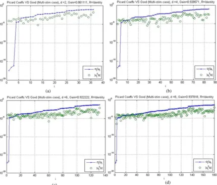
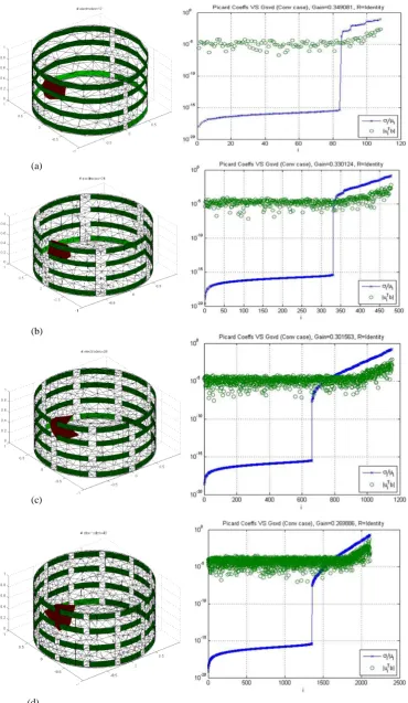
4.5 A comparison between the conventional opposite 2–electrode pair stimulation and multi– injection protocols based on Picard’s stability and GSVD techniques ...63

4.5.1 Conventional opposite 2–electrode pair stimulation protocol – 2D and 3D scenarios ...64

4.5.2 Proposed Multi–injection stimulation protocol – 2D and 3D scenarios ...65

4.6 Multi–injection versus prior information ...74

4.7 Image reconstruction ...77

4.8 Summary ...83

Chapter 5: Conclusions and future work ...84

5.1 The problem and the solution ...84

5.2 Thesis deliverables ...86

5.3 Further Work ...86

References ...89

Appendix A...97

Appendix B ... 107

Figure 1.1 A simple 16–electrodes 2D configuration containing a perturbation. The left– hand side picture shows the single adjacent current injection protocol while on the right– hand side shows opposite multi–injection one. The data collection strategy as shown in the figure is of adjacent nature. That is due to measurements collected from adjacent electrode pairs. ... 2

Figure 1.2 ITS, P2000 Electrical Resistance Tomography System at City University

London. ... 3

Figure 2.1 2D domain, marking clearly the domain W, boundary ¶W, electrodes G_i, and inter–electrodes gaps ¡_j ...13

Figure 2.2 Adjacent method of data collection for a 16-electrode configuration system. For each stimulation pattern, 13 voltage measurements are collected from non-injecting

electrodes (a) First set of injected current I(1) . (b) Second set of injected current I(2). ...27

Figure 2.3 Opposite method of data collection for a 16-electrode configuration system. For each stimulation pattern, 12 voltage measurements are collected from non-injecting

electrodes. (a): First stimulation pattern I(1), (b): Second stimulation pattern I(2). ...28

Figure 2.4 Adaptive method of data collection for a 16-electrode configuration system. For each stimulation pattern, 15 voltage measurements are collected from non-injecting

electrodes. (a): First stimulation pattern I(1) , (b): Second stimulation pattern I(2)...29

Figure 3.1 Groups of Reconstruction algorithms [47] ...39

Figure 3.2 The L–curve of a specific problem, the L–curve is a log–log plot of the solution norm Rx 2₂ versus the residual norm Ax b- 2₂ ...49

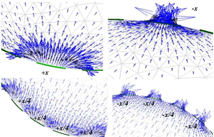
Figure 4.1 Principle of energy conservation. The two top images show the conventional opposite 2–electrode pair injection mechanism, whilst two bottom images show the multi– injection protocol with 4–electrodes per group...58

Figure 4.2 The potential distribution and calculated boundary voltages. (a) The field from the first current pattern for the conventional opposite 2–electrode pair stimulation protocol, (b) the field from the first current patter for the multi–injection protocol with 4

electrodes/group, (c) the measured boundary voltages for the conventional opposite 2– electrode pair stimulation protocol, and (d) the measured boundary voltages for the multi– injection protocol. ...62

Figure 4.3 The current streamlines for (a) the conventional opposite 2–electrode pair and (b) multi–injection stimulation protocols. ...63

Figure 4.4 Conventional opposite 2-electrode pair stimulation protocol gains for a 2D circular medium with a single inhomogeneity located at 2 2 2

(x-0.45) +(y-0.4) -0.2 <0 and

20%

ds = + of the background value. ...67

Figure 4.5 Proposed multi-injection stimulation protocol gains, for a 2D circular test phantom where a single inhomogeneity is located at 2 2 2

(x-0.45) +(y-0.4) -0.2 <0 of

20%

ds = + of the background value. ...68

Figure 4.6 Conventional opposite 2-electrode pair stimulation protocol gains for a 3D cylindrical medium, where a single inhomogeneity is located at

2 2 2 2

(x+0.5) + -(y 0.3) + -(z 0.4) -0.1 <0 ofds = +20% of the background value. A maximum of 3

rings of electrodes are allowed. ...69

Figure 4.7 Multi-Injection stimulation protocol gains for a 3D cylindrical medium, where a single inhomogeneity is located at 2 2 2 2

(x+0.5) + -(y 0.3) + -(z 0.4) -0.1 <0 of ds = +20% of the

background value. A maximum of 3 rings of electrodes are allowed. ...70

Figure 4.9 Proposed multi-injection stimulation protocol gains, for a 3D cylindrical medium, where a single inhomogeneity is located at 2 2 2 2

(x+0.5) +(y-0.3) + -(z 0.4) -0.1 <0 of ds = +20%

of the background value. A maximum of 4 rings of electrodes are allowed. ...72

Figure 4.10 Conventional versus proposed opposite protocol for various numbers n elec_ of electrodes per group per stimulation group. (a) n_elec=1 (Conventional), (b) n elec_ =2, (c)

_ 6

n elec= , (d) n elec_ =8 electrodes per group. The results shown in the left column assume a simple identity prior whilst in the right column, the NOSER prior is used. ...76

Figure 4.11 Conventional opposite protocol. The first column is the original 3D perturbation presented as 2D coronal slices of the cylindrical phantom at levelsh.The columns (2–10) are the reconstructions for various values of the regularisation parameter l

= {1.00000e–001, 1.33352e–002, 1.77828e–003, 2.37137e–004, 3.16228e–005, 4.21697e– 006, 4.62341e–007, 7.49894e–008, 1.00000e–008}, and the last column represents the reconstructed image resulted from the regularisation parameter produced though the L–curve criterion. ...79

Figure 4.12 Proposed opposite protocol (2–electrodes per group). The first column is the original 3D perturbation presented as 2D coronal slices of the cylindrical phantom at levels

h.The columns (2–10) are the reconstructions for various values of the regularisation

parameter l = {1.00000e–001, 1.33352e–002, 1.77828e–003, 2.37137e–004, 3.16228e–005, 4.21697e–006, 4.62341e–007, 7.49894e–008, 1.00000e–008}, and the last column represents the reconstructed image resulted from the regularisation parameter produced though the L– curve criterion. ...80

Figure 4.13 Proposed opposite protocol (6 electrodes per group). The first column is the original 3D perturbation presented as 2D coronal slices of the cylindrical phantom at levels

h.The columns (2–10) are the reconstructions for various values of the regularisation

parameter l = {1.00000e–001, 1.33352e–002, 1.77828e–003, 2.37137e–004, 3.16228e–005, 4.21697e–006, 4.62341e–007, 7.49894e–008, 1.00000e–008}, and the last column represents the reconstructed image resulted from the regularisation parameter produced though the L– curve criterion. ...81

Figure 4.14 Proposed opposite protocol (8 electrodes per group). The first column is the original 3D perturbation presented as 2D coronal slices of the cylindrical phantom at levels

h.The columns (2–10) are the reconstructions for various values of the regularisation

parameter l = {1.00000e–001, 1.33352e–002, 1.77828e–003, 2.37137e–004, 3.16228e–005, 4.21697e–006, 4.62341e–007, 7.49894e–008, 1.00000e–008}, and the last column represents the reconstructed image resulted from the regularisation parameter produced though the L– curve criterion. ...82

Figure A–1 A rough illustration of a 2D with L electrodes attached at its boundary. Right: Continuous domain, and left is the discretised one. ...97

Figure A-2 (a) Linear triangular element in the xy-plane. (b) Linear triangular element in the

ξη-plane. ...98

Figure C-1 2D reconstructions when using conventional opposite 2-electrode pair protocol ... 111

Figure C-2 2D reconstructions when deploying the proposed multi-injection protocol ... 112

Figure C-3 3D reconstructions at different heights when using the conventional 2-electrode pair protocol, a maximum of 3 electrode rings is allowed... 113

Figure C-4 3D reconstruction at different heights when deploying the proposed multi-injection protocol, a maximum of 3 electrode rings is allowed. ... 114

Figure C-5 3D construction at different heights when using conventional 2-electrode pair protocol, a maximum of 4 electrode rings is allowed. ... 115

Table 4.1 Percentage reduction time when using the multi–injection protocol ...62

Table 4.2 Conventional opposite 2–electrode pair stimulation protocol gains for a 2D

circular test phantom. ...73

Table 4.3 Conventional opposite 2–electrode pair stimulation protocol gains, when a

maximum of 3–rings of electrodes is allowed. ...73

Table 4.4 Conventional opposite 2–electrode pair stimulation protocol gains, when a

maximum of 4 rings of electrodes is allowed. ...73

Table 4.5 Multi–injection stimulation protocol gains for a 2D circular test phantom. ...73

Table 4.6 Multi–injection stimulation protocol gains, when a maximum of 3 rings of

electrodes is allowed. ...73

Table 4.7 Multi–injection stimulation protocol gains, when a maximum of 4 rings of

electrodes is allowed. ...73

Throughout the thesis, column vectors and matrices are identified in bold upper–case

letter, whereas continuous functions are identified in italic letters. The ( , )i j thentry of matrix A isA_ij, similarly the ithentry of a vector x is x_i.

W modelled body

¶W medium boundary

Ñ del operator

B magnetic flux density

H magnetic field intensity

r charge density

m _{magnetic permeability}

D electric flux density

E electrical field intensity

j current density inside a medium (continuous function)

j total current density inside the medium, it is the summation of the

conduction and source current densities i.e., j = j_c+j_s

J the Jacobian or sensitivity matrix

L nonlinear forward operator that maps the change in the interior

conductivities onto the change in the collected boundary voltage

measurements

s conductivity distribution (continuous function)

s _{vector containing discrete conductivity values (the entries}

1,.., k k= K s

represents conductivity values at the faces of simplices composing the

discretised medium)

ds vector containing the change in conductivity values with respect to a

reference conductivity s₀

ˆ

n outward unit normal

( ) i

f discrete values of electrical potential at the nodes of the simplices

e electrical permittivity or at some locations is additive noise

w relaxation parameter in Landweber iteration

G union of electrodes G_l

l

G area (in 3D) or length (in 2D) of thelth electrode

l

z contact impedance of thelth electrode

l

V electric potential at thelth electrode

y _{boundary measured voltages as a function of conductivity change}

y _{vector containing the finite boundary measured voltages}

fwd

y vector containing the finite boundary voltages calculated via FEM

dy vector containing the change between the measured and calculated boundary

voltages

n number of nodes in the mesh

I current pattern

K number of elements in the mesh

a regularisation parameter

d change in a given quantity

D an update in a given quantity mainly used in iterative formulae

( ) ( )

n n

t

¶ ¶

nth partial derivative with respect to time

L total number of electrodes

m number of voltage measurements collected at the medium’s boundary

g _{generalised singular values}

h levels at which the 3D model is sliced (for visualisation purposes)

D[.] a given operator applied to a function

( )

R x residual function

Abbreviation Meaning

CEM Complete Electrode Method

CG Conjugate Gradients

CG Conjugate Gradient

CT Computer Tomography

EIT Electrical Impedance Tomography

FEM Finite Element Method

GSVD Generalised Single Value Decomposition

MRI Magnetic Resonance Imaging

PCG Preconditioned Conjugate Gradient

PDE Partial Differential Equation

PET Positron Emission Tomography

SPECT Single Photon Emission Computerised Tomography

STR Standard Tikhonov Regularisation

SVD Singular Value Decomposition

TGSVD Truncated Generalised Singular Value Decomposition

Introduction

Research is to see what everybody else has seen, and to think what nobody else has thought

Albert Szent–Gyorgyi

1.1 Electrical Impedance Tomography (EIT)

Electrical Impedance Tomography (EIT) has been a topic of increasing interest to the

Medical Imaging community in the last few decades. Since 1970s, EIT has been

actively researched where the number of published papers and journals has been

notably growing. As the name suggests, EIT is the process of producing 2D and 3D

images of the inside of a medium. This process takes place through injecting a given

medium with a sequence of electrical currents via an array of electrodes attached to

its periphery, and measuring the resulted voltages. These measurements are then used

to reconstruct visual images of the inside of that medium.

The non–invasive nature of the EIT technology, its practicality and portability in

producing images have shown promising results which may lead to adopting this

technology in medical or industrial applications.

One advantage that distinguishes EIT from other imaging modalities is the use of

low–amplitude AC currents in the injection process. Although for some, this is

considered a disadvantage during to the scattering effect [1], but for others, it is an

advantage due to low power (heat) injected into the medium especially when used for

medical purposes and the medium is the human body.

The set of electrodes, either current–injecting or voltage–measuring, can be arranged

in different ways to achieve the best rate of object detection or distinguishability.

electrical currents are fired into the medium and voltages are measured across

various electrodes at the boundary. Figure 1.2 shows the ERT (Electrical Resistance

Tomography) system used in the Information Engineering and Medical Imaging

[image:16.595.136.506.170.339.2]

Centre at City University London.

Figure 1.1A simple 16–electrodes 2D configuration containing a perturbation. The left–hand side picture shows the single adjacent current injection protocol while on the right–hand side shows opposite multi– injection one. The data collection strategy as shown in the figure is of adjacent nature. That is due to measurements collected from adjacent electrode pairs.

Historically, the 2D EIT has suffered from producing limited spatial resolution due to

its ability to only produce a cross sectional image of a 3D medium let alone the

limitation in the electrodes configuration. Both make the 2D EIT modality less

resembling to real life problems. However, the application of 3D EIT through

employing two or more equally spaced electrodes sequence around a body in specific

planes has introduced enhancements in the reconstructed images as reported in [2]

and [3]. The use of EIT imaging modality in many applications such as biomedical,

industrial, geophysical, etc., is almost the same; that is due to the image

reconstruction process, which differs only in the use of the prior information and the

[image:17.595.221.427.83.236.2]

Figure 1.2 ITS, P2000 Electrical Resistance Tomography System at City University London.

It is important to note at this stage that images produced from deploying the EIT

modality are of a differential nature i.e., imaging the impedance difference between

two states; the reference state which depicts our prior knowledge of the medium, and

object/phantom which lies/occurs within that medium. This narrows down the EIT

applications to moving objects or 2–state phantoms only, e.g., moving objects in a

medium or the inhale and exhale process of the lungs. Other EIT modalities have

been developed such as the Multi–frequency EIT which entails injecting the medium

with electrical currents of various frequencies, this is outside the scope of this thesis.

To achieve this, the medium is first injected with reference electrical currents and

voltage measurements are then taken from the boundary. Another set of

measurements are collected at a different state of medium (when the resistive change

takes place). Using the difference in voltages and currents, an image is then

reconstructed to represent the change in medium’s resistivity. Therefore, EIT can be

widely used in many medical applications based on difference imaging such as, the

gastric imaging, detection of intrathoracic fluid volumes, detection of haemorrhage,

and monitoring of hyperthermia.

The EIT modality along with many imaging applications are a part of class of

problems referred to as inverse problems. These problems generally arise when one

wishes to compute information about internal or otherwise hidden data from the

external (or otherwise accessible) measurements. Inverse problems, in turn, belong to

the class of ill–posed problems. The term was coined in the early 20th century by

Hadamard who worked on problems in mathematical physics, and believed that ill–

posed problems did not model the real world, however, he proved to be wrong.

Hadamard defined a linear problem to be well–posed if it satisfied the following

three requirements [5]:

· Existence: the problem must have a solution

· Uniqueness: there must be only one solution to the problem

· Stability: the solution must depend continuously on the data

If a problem violates one or more of these requirements, it is said to be ill–posed.

The EIT problem involves estimating the unknown material conductivity distribution

s from the collected boundary measurements y. Clearly, this problem is nonlinear;

therefore, one can introduce a forward operator L as

( )s y

L = Eq.(1.1)

where s is the medium’s conductivity distribution and y is the observable

boundary measurements vector. However, in order to solve this system, one opts to

discretise Eq.(1.1), using Taylor’s expansion for example, and yields the following

discrete linearised system

¶ = ¶

J s y Eq.(1.2)

where J is the discrete form of the operator L _{(Jacobian or sensitivity matrix),} ¶s

is the finite number of conductivities across the faces of the simplices comprising the

model, and ¶y is the finite number of collected boundary voltage measurements. (A

thorough discussion of the linearised EIT inverse problem is discussed in the

following chapters).

Generally speaking, the relatively poor spatial resolution of the reconstructed images

imaging techniques with good resolution. In this respect, it must be clarified that the

motivation of EIT is somewhat different from that of conventional imaging

techniques. Despite its limited resolution, the main ask is to provide a reliable, real–

time, portable and cost efficient imaging tool. However, the process of conductivity

estimation in EIT is a highly nonlinear, ill–conditioned1 and ill–posed problem. The

sensitivity matrix J, which relates interior conductivity difference to perturbations in

the boundary voltage data is heavily ill–conditioned with respect to inversion. So, it

requires special treatment in the form of regularisation or a truncation of a singular

value expansion [5]. When approaching an ill–posed problem, instead of attempting

to solve the original problem one often opts to solve a similar one which is less

computational exhaustive. Therefore, effective EIT image reconstruction algorithms

are required.

1.3 The toilsome EIT

As mentioned earlier, the problem of recovering an unknown conductivity

(reciprocal of resistivity) from boundary data is severely ill–posed, and it is

Hadamard’s third criterion which is violated. In practice, for any given measurement

precision, there are randomly large changes in the conductivity distribution which are

untraceable by boundary voltage measurements at that precision. This is a direct

indication that low frequency electrical imaging does not provide an accurate

conductivity change and boundary voltage correlation. However, the ‘partial’

solution of this problem is to incorporate additional information about the

conductivity distribution. When sufficient prior information is known, it limits the

solution so that the huge variations causing the instability are eliminated.

Further, the first two Hadamard’s requirements can be overcome more easily than the

third; as the existence of a solution is not an arguable issue. That is due to the fact

that the body naturally does have conductivity on the inside. The catch here is that,

the data should be sufficiently accurate to be consistent with the conductivity

1

distribution. Minute errors in measurement can violate consistency conditions, such

as reciprocity. One of the ways to overcome this problem is to project this unviable

data onto the closest viable set. Finally, the problem of solution uniqueness is often

referred to by mathematicians as sufficiency of data [5].

Generally speaking, the conductivity inverse boundary value problem (or

Calderónproblem) is to establish a complete knowledge of the relationship between

voltage and current at the boundary and to determine the conductivity in a unique

manner. This has been demonstrated under a variety of assumptions about the

smoothness of the conductivity [6]. However, since only a finite number of

measurements from the electrodes can be collected, and since the electrodes cover

only a portion of the surface of the body, and not all of them are involved in the

measurement process, the number of independent measurements made and the

accuracy of the measurements limit the number of degrees of freedom of a

parameterised conductivity that one can recover.

1.4 EIT hardware

Most of the factors limiting measurement accuracy in EIT systems lie with the data

acquisition system. In most practical systems, the measuring device applies a known,

current pattern on two or more electrodes, and measures the developed voltages

across the others. As reported in [7], a practical EIT system will normally have the

following components: waveform synthesiser, current source, differential amplifier,

and a demodulator or some combination of their components. A comprehensive

discussion on EIT hardware components can be found in [7] and [8]. Rigaud and

Morucci [8], [9] published a review on the hardware solutions developed for EIT and

outlined the progress which has taken place in recent years, in terms of measurement

strategy and development to overcome hardware error sources that have undesired

effects on image recovery [8]. In effect, it appears that there are significant

instrumentation problems, due to the interaction of finite current drive output

impedance, recording amplifier common mode rejection, and unequal skin–electrode

impedances. A number of different EIT systems were successfully constructed or are

employ varying strategies, such as additional electrodes, multiple electrode current

injection, or recording at multiple frequencies, to improve image accuracy with great

success.

1.5 EIT as an imaging modality

There are currently three ways to image the distribution of impedance within the

body [7], according to the nature of the application: static, multi–frequency or

dynamic corresponding to single frequency, multi–frequency and “real–time”

imaging types. The first two ways are normally concerned with producing images

that show how the different types of tissue are distributed in the body, known as

tissue characterisation or anatomical imaging. In such applications, EIT is used as an

alternative to X–rays, CT and MRI, with certain practical advantages. The third

technique produces images of physiological function, such as imaging short (e.g.,

millisecond) changes in the physiological state of the body.

In electrical impedance tomography, images are reconstructed from sets of electrical

measurements made on the surface of the body. To obtain high–quality images,

independent measurements with good accuracy, precision and repeatability are

needed from the data acquisition system. Noise, optimal current patterns, and

electrode–electrolyte impedance are among other factors that impose stringent

requirements on the accuracy of an EIT data acquisition system. Despite these

hurdles, useful images at relatively low resolution have been obtained. In [3], a

spatial resolution of about 10% of image background for a centrally located object in

the cross–sectional plane, using a 64–electrode data acquisition system is reported.

Using a 32–electrode system, Casas et al [12] obtained a spatial resolution of 14%

for a similar scenario. Although, the spatial resolution of EIT is limited, its temporal

resolution and sensitivity in dynamic imaging is rather good [13]. It appears that

better spatial resolution ought to be achievable by improving either the data

acquisition system and/or the performance of the reconstruction algorithm [14].

One of the downfalls of EIT is its limited spatial resolution of the conductivity

distribution on the inside of a conductive continuum. However, the addition of a third

dimension, has added the flexibility needed to add more electrodes, and therefore,

more measurements to be incorporated in the reconstruction process. Indeed, that

helped to capture the conductivity distribution from different axes and angles, but

added an exhaustive process in acquiring the measurements resulted from increasing

the number of injecting electrodes.

Therefore, the aim of this thesis is to develop enhancements in EIT current injection

protocols, reducing the acquisition time, whilst maintaining the quality of the

produced EIT images. The aim of this thesis will be addressed in terms of the

following objectives:

1. Utilising the concept of multi–injection protocol over 2D shapes, and

comparing it against the existing opposite 2–electrode pair stimulation

protocol in terms of quality and acquisition time.

2. Extending the concept to cover 3D shapes, with different levels of electrode–

rings, and comparing the quality based on the gain of the selected stimulation

pattern quantifier, that is, the ratio of the generalised singular values that meet

Picard’s criterion [15] over the total number of available generalised singular

values.

3. Assessing the effect of deploying the multi–injection protocol on the quality

of the resulting reconstructed images.

In the EIT forward model simulations, high–resolution fine meshes generated by the

Netgen mesh generator [16] are developed. The numerical costs associated with this

can be dealt with quite easily due to the use of Finite Element Analysis (FEA) to

solve the forward problem. On the other side, for the inverse problem, coarser

meshes are generated using the same platform, and that is for two reasons, the first is

to avoid the so–called inverse crime resulting from employing the same model to

generate, as well as invert, the given data [17], while the other reason is to ease off

the inverse calculations due to calculating the inverse of the Jacobian matrix whose

model. Finally, throughout the simulations carried out in this thesis, it is assumed

that the voltages are not measured on the current carrying electrodes, e.g., [18]–[19].

1.7 Thesis contribution

This work done has contributed to the Electrical Impedance Tomography imaging

technology by adding an adjustment to the current injection and voltage

measurement processes. The thesis scope is a follow up to the guidelines of the work

done in [20], in which the authors have made use of deploying multi–current

injection patterns over 2D mediums. This has produced a lesser number of collected

measurements and therefore reduced computational overheads when solving the

forward problem.

In addition, the thesis extends the scope to include 3D models, where a greater

number of electrodes and patterns is often available. The work develops the 3D

multi–current injection stimulation pattern; that is, injecting alternating electrical

currents through selected opposite groups of electrodes instead of injecting through

only a pair.

On the other hand, the contribution of this work differs from the one in [20]; in this

work, the groups of variable electrode numbers to apply the desired stimulation

protocol are accounted for. This implies a variable reduction in the number of

collected measurements (and thus data acquisition times) without compromising the

quality of the reconstructed images.

A detailed overview of the EIT forward model including the various interpretations

of electrode–boundary interactions, the solution of the governing Laplacian equation,

and the formulation of the EIT forward and inverse problems and the derivation of

the Jacobian matrix are encapsulated in Chapter 2.

Afterwards, Chapter 3 proceeds with illustrating the inverse nature of the EIT

problem, and the various techniques and methods used to solve the linearised EIT

inverse problem. It also discusses the concept of regularisation, and different

methods, direct or iterative, to perform the regularisation process over the EIT

problem. A quantifier referred to as the Discrete Picard condition, to assess the

performance and robustness of an EIT system under the existence of noise is

discussed.

Chapter 4 sets out the simulation framework as it starts off with a demonstration of

the multi–injection protocol in 2D models, which is expanded to cover 3D ones.

Picard graphs and image reconstructions quantifying the performance of each

stimulation protocol including the gain calculations are also presented within. The

thesis finally concludes with Chapter 5 which contains the conclusions and any

The EIT forward problem

Research is what I’m doing when I don’t know what I’m doing.

Wernher Von Braun

In this chapter, the formulation of the EIT forward problem is derived from the basic

principles of Maxwell’s equations. This is followed by a discussion of various

electrode configurations and current injection/voltage acquisition protocols used

throughout the history of EIT. Afterwards, the study expands to cover the use of

some of the common analytical and numerical methods to solve such equations. The

emphasis will be applied on the use of the Finite Element Method (FEM) which

benefits and downfalls will be highlighted. Finally the chapter concludes with the

derivation of the EIT inverse problem and the associated system which, along with

other factors, accounts for the image reconstruction problem discussed in the

following chapter.

2.1 Overview of the forward problem

In order to produce meaningful images of the interior of a given conductive medium

with an object/phantom lying/occurring within, two interconnected and subsequent

processes are considered; The forward problem; where one opts to estimate the

boundary voltages excited across the boundary electrodes as a result of injecting the

medium with a specific electrical current pattern. The second process, which is

referred to as the Inverse problem, is the process in which the mathematically

calculated voltages along with the experimentally are used to find an estimation of

the difference of the medium’s inner conductivity in a form of an image.

Mathematically speaking, assuming a uniform medium with homogenous

conductivity distribution, continuous boundary and a known current pattern driven at

fwd m

Î

y ¡ , where m is the number of voltage measurements across boundary

electrode.

This includes solving the governing Laplacian equation,

( ) ( )

(

)

. s f 0

Ñ x Ñ x = Eq.(2.1)

where f

( )

x ÎH1

( )

W 2 [1] is a scalar function representing the electric potential inside the continuum, s

( )

x ÎL2

( )

W 3

is the material conductivity (real material

conductivity is assumed throughout). Both the electric potential and conductivity are

functions of the spatial distribution xÎW and the body W Ì¡n

which is a closed

and bounded subset of a 2D (i.e.,n = 2) or 3D (i.e., n= 3) space with a smooth (or

sufficiently smooth) boundary ¶W. Figure 2.1 illustrates a simple 2D medium

configuration.

For Eq.(2.1) to be solved uniquely, one ought to couple it with a set of boundary

conditions that represents restrictions imposed on the problem at hand, such as

smoothness of the boundary or confinement of energy. This can be achieved by

either deploying analytical [21], i.e., calculating the potentials at any points inside a

given medium, or numerical solutions [22], i.e., which find estimates of the

potentials at the nodes of the finite elements composing the model. Through the

course of EIT history, numerical techniques have proved to be superior over the

analytical ones, due to their adaptability to complex geometries, which the analytical

techniques have shown to be very computationally exhaustive in dealing with.

However, another important factor in solving Eq.(2.1) is the accurate modelling of

the phantom under study. This includes the geometry and boundary of the model.

2

Having the electrical potential f

( )

x to be in the Sobolev space i.e., f

( )

x ÎHk

( )

W for an integer

k indicates that the square of thekth derivative has a finite integral over the domain W . For non-integer and negative powers, Sobolev spaces are defined by taking the Fourier transform, multiplying by a power of frequency and demanding the result is square integrable i.e., ( )

2

( )k d

f

W

W < ¥

ò

x .

3

The locations of the electrodes on the surface are also of prime importance; their

characteristics might affect their reliability and applicability in real life applications.

In the next section, Maxwell’s equations are used as mathematical links which tie the

conditions imposed over the medium’s boundary with the electrical fields inside the

[image:27.595.168.476.199.467.2]

medium.

Figure 2.1 2D domain, marking clearly the domain W, boundary ¶W, electrodesG_i, and inter–electrodes gaps ¡_j

2.2 EIT problem formulation

In this section, Maxwell’s equations for electro–magnetics [23] are used to derive the

generic EIT governing Equation Eq.(2.1). Without loss of generality, the medium is

assumed to be uniform, conductive, isotropic, non–dispersive, and linear. The current

injection is confined within the electrodes’ areas and is normal to the boundary ¶W.

The electrodes are assumed as disjoint uniform boundary segments (as shown in

Figure 2.1). There is no current traffic on the inter–electrode areas (labelled as ¡_l in Figure 2.1). Finally, the eddy (leakage) currents will be assumed zero, i.e., the

amount of currents injected into the medium is exactly equal to the amount exiting.

Further, Maxwell’s equations state that the curl of the electrical field intensity

E

is equal to the negative time–derivative of the magnetic flux densityB,

t ¶ Ñ´ =

-¶ B

E Eq.(2.2)

and that the curl of magnetic field intensity H is essentially the current density

flowing inside the medium plus the rate of change of the electric flux densityD, as

t ¶

Ñ´ = +

¶ D

H j Eq.(2.3)

where E, B, H, D, and j refer to the electric field intensity, magnetic flux density, magnetic field intensity, electric flux density, and current density, respectively.

From Gauss’s law for magnetism, the divergence of

B

through a closed surface is

equal to zero i.e.,

. 0

Ñ B= Eq.(2.4)

and according to Gauss law, the charge density

r

can be given as the divergence of

Das,

. r

Ñ D= Eq.(2.5)

The conduction current density can be represented as

c =s

j E Eq.(2.6)

However, the total current is then j= +j_c j_s, the sum of the conduction and source currents. EIT assumes that the source current j_s is typically zero at frequency w .

EIT assumes that the injected electrical currents are of a low frequency nature, in

which a change in conductivity would have some effect on any measurement of

surface voltage [24]. This assumption makes it possible to neglect the magnetic field

effects or simply assuming a direct current case.

Hence, taking the divergence of Eq.(2.3) as,

(

)

. .

t ¶

æ ö

Ñ Ñ ´ = Ñ _ç + _÷

¶

è ø

D

H j Eq.(2.7)

(

)

. . . 0

t

¶

Ñ Ñ´ = Ñ + Ñ =

¶

H D j Eq.(2.8)

Substituting Eq.(2.5) into Eq.(2.8) results in,

. 0

t

r ¶

+ Ñ =

¶ j Eq.(2.9)

Since the system is assumed to be running under the quasi–static assumption, the

term

t

r

¶

¶ therefore plunges to zero, resulting in,

. 0

Ñ =j Eq.(2.10)

Eq.(2.10) is another way of looking at Kirchhoff’s current law; the amount of the

current going into the medium is the same as the amount of currents going out

(conservation of energy). Using relation j_c =sE, Eq.(2.10) can be rewritten as

( )

(

(

)

)

(

)

.

s

0 .

s

f

0 . 0

s f

Ñ E = Þ Ñ -Ñ = Þ Ñ Ñ = Eq.(2.11)

2.3 Electrode models

As previously mentioned, in order to solve Eq.(2.1) efficiently, a set of boundary

conditions ought to be incorporated. Through the history of EIT, several electrode

configurations demonstrating these conditions have been developed in order to

interpret the electrode interactions with the medium to which they are attached. A

detailed description can be found in [25].

Throughout the thesis, unless otherwise stated, the electrodes are considered as a set

of disjoint boundary segments G_l where

1 L

l l=

G =

U

G ;L is the total number of electrodes Eq.(2.12)

represents the total boundary segment occupied by the electrodes with each having a

length (2D shapes) or an area (3D shapes) of G_l units. On the other hand, the

boundary segments denoted by ¡_l where

1

\ L

l l=

characterises the total inter–electrode boundary gaps.

2.3.1 Continuum Electrode Model

The continuum electrode model [26] is the simplest of the models used in electrical

impedance tomography. This model does not account for the attached electrodes, and

assumes that the injected current is a continuous function, that is,

( )

( ) cos

I t =

u

wt _Eq.(2.14)

where u and w are the constants corresponding to current amplitude and frequency,

respectively.

Hence, according to the continuum model, the injected current density can be

randomly set on the entire boundary of the medium

ˆ ˆ

. .

int = - inj

j n j n on ¶W _Eq.(2.15)

where nˆ is the outward normal vector to ¶W, and j_inj is the injected current density.

This configuration only considers the normal components of the injected current, as

electrodes (supposed to be perfect conductors) would shunt the tangential

components of the electric field. Using Ohm’s law and recalling that E is

conservative, Eq. (2.15) can be expressed as a Neumann boundary condition

ˆ .

ˆ inj

f s ¶ =

-¶n j n on ¶Ω Eq.(2.16)

Additionally, the conservation of charge must be preserved

( )

ˆ

. .d 0

inj ¶W

¶W =

ò

j n Eq.(2.17)

and the condition

( )

.d 0

f

¶W

¶W

ò

= Eq.(2.18)

to make the model complete by assigning a reference voltage. The continuum model

is a very rough approximation of the electrode/medium interface and hence, the

difference between the voltages resulting from the forward calculations and the

2.3.2 Gap Electrode Model

The Gap Electrode Model [24] is an enhancement of the previously described

continuum model. It is the first model to consider the electrodes as a set of discrete

subdomains (as shown in Figure 2.1), and it approximates the current density at each

electrode by a constant value

on for 1,...,

ˆ

0 on for 1,...,

l

l l

l

l

I

l L

j

l L

f s

ì _{G =}

¶ _{ï G}

= _{= í}

¶ _ï

¡ =

î

n Eq.(2.19)

where I_l is the injected current atlelectrode The conservation of charge is imposed as

0 l l

I =

å

Eq.(2.20)

Unfortunately, the assumption that the current density is constant on the interface of

each electrode is an oversimplification for many practical EIT applications.

Moreover, both the continuum and gap models ignore both the shunting effect of the

electrodes and their contact impedances.

2.3.3 Shunt Electrode Model

The Shunt Electrode Model [24] modifies the Gap Electrode Model by considering

that the current density characteristics underneath the electrodes are assumed to be

unknown. The model simply assumes that the total current density injection through

the electrodes should be equal to the injected current. This means replacing the

condition in Eq.(2.19) by

ˆ

j=s ¶f

¶n on G Eq.(2.21)

The main difference from the gap model is that the shunt model accounts for the

shunting effect i.e., considering the potential at each electrode to be constant as

( )

l Vl

f

G = Eq.(2.22)

As mentioned earlier, V_l represents the electric potential value at thelth electrode.

0 l l

V =

å

Eq.(2.23)

However, this model underestimates the resistivities, since it ignores the contact

impedance of the electrodes.

2.3.4 Complete electrode model

The complete electrode model (CEM) [27], [28] is the most refined description of the

interface between the electrodes and the boundary of the medium. The model is an

update of the Shunt Electrode Model as it includes the effect of the contact

impedance with the boundary.

The alternating currents are fired from a set of electrodes fixed at the periphery in a

direction normal to the boundary surface. This gives arise to a current density j of

ˆ

j=s ¶f

¶n on G Eq.(2.24)

and since the injection is limited to the electrodes, the inter–electrode gaps exhibit no

flow of current through them. Also, the eddy currents escaping these areas are

assumed to be negligible,

0 ˆ

f s ¶ =

¶n on

¡

Eq.(2.25)

Finally, what differentiates the complete electrode model from its predecessors is its

consideration of the voltage drop across the thin layer (resistance) connecting the

electrode to the medium. Mathematically speaking,

ˆ

l l

z f V

f+ s ¶ =

¶n on Gl Eq.(2.26)

where z_l ¹0 is the electrode contact impedance which could vary over G_l but

assumed constant i.e., z_lΡ. Another way of writing the expression in Eq.(2.26) is

ˆ .

l l

z V

f+ s fÑ n= on G_l

It has been proven in [27] that this model produces a unique solution when the

conservation theorem hold, i.e.,

1 0 0 L l l I ¶W =

= Û

å

=

ò

j Eq.(2.27)

1

0 0

L l l

V

f

¶W = Û

å

₌ =

ò

Eq.(2.28)

The Complete Electrode Mode is a well–posed problem and has a unique solution. It

is also the most refined electrode model in EIT so far.

2.4 Finite Element Methods in the solution of solving the EIT

forward problem

In order to solve for the electrical potentials and boundary voltages, the governing

equation in Eq.(2.1), along with a boundary condition selection (as described in

Section 2.3.4) are coupled together to construct an integrated system which, with the

aid of discretisation, turns into a linear system of equations that can be solved either

via direct or iterative methods.

The basic idea of Finite Element Methods (FEM) [29] is to approximate the domain

of interest

W

as a union of a finite number of elementsW_k, which for simplicity can be assumed to be simplices. In a two dimensional scenario, a simplex is a triangle,

and in a three dimensional one, it is a tetrahedron. A collection of such simplices is

called a finite element mesh.

Assuming a domain W having K simplices with n vertices. The continuous

electric potential

f

( )

x inside the mesh i.e., xÎW can be approximated using this mesh by functions, which are linear on each simplex, and continuous across the

faces. These functions, also referred to as interpolation or basis functions, have the

appealing feature that they are completely determined by their values at the mesh

vertices. A natural basis is the set of functions N xi

( )

that are one on vertex

i

and

zero at the other vertices, i.e.,

( )

1 on vertex ,

0 otherwise.

i

i

N = íì

î x

( )

( )

( )

1

( )

( )

1 1 2 2 n

i i i

n n

N

N N N

f f j

j j j

=

@ =

@ + + +

å

x x

x x x

%

L

Eq.(2.29)

and the vector [ ,...,j₁ j_n]T Ρn represents the discrete approximations of the electric potential.

However, it is not difficult to note that these basis functions have to be either

quadratic or at least twice differentiable in order satisfy equation Eq.(2.1) [1] due to

the second order derivative nature of the Laplacian operator. However, the resulting

complexity resulting from using such basis functions can be avoided by utilising a

method referred to as TheMethod of Weighted Residuals (MWR) [30], the latter will

be elaborated in more details in the following sections.

2.4.1 Continuous domain setting

The forward problem under consideration, in this context, is the one described by

Eq.(2.1), and the set of boundary conditions Eq.(2.24) – Eq.(2.28). As mentioned

before, in order to apply the finite element concept and discretise the system, the

weak formulation of the problem should be derived first.

2.4.1.1 Weak formulation of the EIT Partial Differential Equation

(PDE)

Many authors refer to the PDE described by Eq.(2.1) as thestrong formulation. This

is due to the fact that in order to solve this equation, one must be able to compute the

highest order derivative term in the PDE. In other words, the electric potential

function

f

( )

x must be at least twice differentiable and should not disappear when its second derivatives are taken. Hence, one way to weaken this requirement, integration

by parts can be applied to the strong formulation to derive the weak formulation of

the problem. The weak formulation, therefore, allows the use of the first–order linear

The Method of Weighted Residuals or MWR [30] is a family of methods mainly

used to obtain approximate solutions to differential equations. Mathematically

speaking, if one assumes a linear operator D acting on a potential function f( )x to produce a function p x( ),

[

( )

]

( )

D f x = p x

and the function f( )x is to be approximated as in Eq.(2.29). Then, by substituting the discretised value of f( )x , i.e., f% into the differential operator, D, does not, in general, result in p x( ). Hence, an error or residual exists,

( )

( )

0

R x =Dé ù_{ë û}f% -p x ¹

The idea behind the method of weighted residuals is to essentially force the residual

function to zero in some average sense over the domain W, i.e.,

( ) ( )

0, 1, 2,...,

w R d i n

W

W = =

ò

x x Eq.(2.30)

where w x( ) is the weight function.

In this context, for the EIT forward problem governing equation, the function p x

( )

is zero, and denoting the Laplacian in Eq.(2.1) by Dé ù_{ë û}f% and residual function R x

( )

in Eq.(2.30) is essentially

( )

( )

(

)

(

)

. 0 .

R D f p

s f s f

é ù = _{ë û} -= Ñ Ñ -= Ñ Ñ

x % x

Eq.(2.31)

Therefore, inserting this result into Eq. (2.30), results in

(

. ( )

)

0

w s f

W

Ñ Ñ =

ò

on

W

Eq.(2.32)

Using Green’s second identity and the vector identity

(

)

(

)

. w

s f s f

. w w .

s f

Ñ Ñ = Ñ Ñ + Ñ Ñ Eq.(2.33)

Eq.(2.32) changes to

0 from equation (2.32) . (ws f) d s f . w d w .(s f)d

W W W

=

Ñ Ñ W = Ñ Ñ W + Ñ Ñ W

ò

ò

ò

1442443

Eq.(2.34)

Invoking the divergence theorem

(

)

(

)

ˆ

. ws f d ws f dS .

W ¶W

Ñ Ñ W = Ñ

and given that the current density is zero outside the electrodes, as in Eq.(2.25), yields, ˆ .( ) . ˆ .

w d w dS

w dS

s f s f

s f

W ¶W

G G

Ñ Ñ W = Ñ

= Ñ

ò

ò

ò

n n Eq.(2.36)

Eq.(2.32) can be rewritten using the observation of Eq.(2.36) as,

ˆ

. w d w dS .

s f s f _G

W G

Ñ Ñ W = Ñ

ò

ò

n Eq.(2.37)

Rearranging the boundary condition in Eq.(2.26) gives,

(

)

1 ˆ . _l l V z

s fÑ n= -f on

G

Eq.(2.38)

where z_l ¹0 is the contact impedance between the electrode and medium boundary.

Therefore, incorporating Eq.(2.38) into Eq.(2.37) gives,

(

)

1 1 . l l L l l l

w d V w dS

z

s f f _G

=

W G

Ñ Ñ W =

å

-ò

ò

Eq.(2.39)

or more conveniently,

1 1

1 1

. 0

l l

l l

L L

l

l l l l

wd wV dS w dS

z z

s f _G f _G

= =

W G G

Ñ Ñ W -

å

+

å

=

ò

ò

ò

Eq.(2.40)

Finally, the injection current into the medium has the constraint

ˆ l

l

l

I s fdS_G

G

¶ =

¶

ò

_n Eq.(2.41)

which indicates that the amount of current injected into the medium can be kept at

certain values through controlling the voltages at the boundaries. This is beneficial

when using EIT in medical applications and excessive current values might lead to

tissues damage.

Eq.(2.40) is the weak formulation of the governing boundary value problem of

Eq.(2.1) with current density applied through the electrodes.

In addition, if the weight functions w x

( )

are chosen from the same set of functions as the basis functions N xi

( )

, i.e.,

( )

( )

for 1, 2,...,

the featured weighted residual method is referred to as the Galerkin method [30].

The Galerkin method is discussed in the context of this thesis rather than the

variational approach due to its simplicity and its intuitive interpretation. The use of

variational methods in the solution of boundary value problems is discussed in [31]–

[33] and the references therein.

2.4.2 Discrete domain setting

Next, we discuss the process of discretising the weak formulation of Eq.(2.40). That

is, computing the solution over a given medium with smooth predefined boundaries.

This is done by discretising the domain into a collection of subdomains and

calculating the electrical potentials across the nodes (connectors) of these

subdomains.

In order to do so, we follow the Galerkin approach by choosing the weight and basis

functions to be from the same family. Hence, the weak formulation of Eq.(2.40) turns

into,

1 1 1

1 1

0

l l

l l

n L L

i j i i j i i l

i l l l l

N N d N N dS N dS V

z z

s j _G j _G

= W = G = G

ì ü ì ü

ì ü _{ï ï ï ï}

Ñ Ñ W + - =

í ý í ý í ý

î þ ïî ïþ ïî ïþ

å

ò

å

ò

å

ò

Eq.(2.43)

and from Eq.(2.41), the current injected from each exciting electrode can be

represented as,

(

)

1 1 1 1 1 1 1 l l l l l l l l l l n

l i i

i

l l

n

l l i i

i

l l

I V dS

z

V dS N dS

z z

V N dS

z z f j j G G G = G G G = _G = -ì ü ï ï

= - _{í ý}

ï ï

î þ

ì ü

ï ï

= G - _{í ý}

ï ï î þ

ò

å

ò

ò

å ò

Eq.(2.44)

where Gl is the area (or in two dimensions, length) of thel th

electrode.

If IΡL is the vector containing a current pattern, then another vector _bΡn L+ _can

conductance or stiffness matrix with entries indicated below, then using Eq.(2.43)

and Eq.(2.44) the EIT forward problem can take the form of a linear set of equations

as [1]

=

Ax b Eq.(2.45)

where M _T Z W n L n L

W D + ´ + + é ù Î ê ú ë û

A A A

A =

A A ¡ having the entries:

M

A is an n n´ symmetric matrix, and has entries A_{Mi j,} ,

, . for , 1,...,

Mi j s Ni N dj i j n W

=

ò

Ñ Ñ W =

A Eq.(2.46)

which represents the solution of Eq.(2.1) discarding all boundary conditions.

However, the conductivity distribution s is to be approximated over the mesh. An

intuitive method is to choose s to be constant on each simplex (e.g., piecewise

constant (PWC) [1]).

Assuming c_i to be the characteristic function which has the value of one on the jth

simplex and zero elsewhere, we have an approximation to s

1 K j j j s c = »

å

s Eq.(2.47)

whereK is the total number of subdomains consisting the medium.

The constant s_j can be taken outside the integral for each simplex. Therefore,

Eq.(2.46) can be rewritten as,

, 1

.

k

K

Mi j k i j k k

N N d

s

= W

=

å ò

Ñ Ñ W

A Eq.(2.48)

The matrix A_Z is ann n´ matrix that has entries A_{Z i j,}

, 1

1

for , 1,..., and 1,...

l l

L

Z i j i j l l

N N dS i j n l L

z G

= _G

ì ü

ï ï

= _{í ý} = =

ï ï

î þ

å ò

A Eq.(2.49)

Furthermore, the matrix A_W is an n L´ matrix having entries A_{Wi j,} , 1

for 1,..., and 1,...

l l

Wi i

l

N dS i n l L

z G

G

= -

ò

= =

and matrix A_D is an

L L

´

diagonal matrix, having entries , 1 , for , 1,..., 0, otherwise i j l l D j i j

z i j L

ìæ ö

G =

ïç ÷

=_{íè ø} =

ï î

A Eq.(2.51)

Hence, Eq.(2.45) can be rewritten including the previous components as,

M Z W

T

W D

+

é ù é ù é ù

=

ê ú ê ú ê ú

ë û ë û

ë û

A A A 0

A A V I

F

Eq.(2.52)

and solved for the approximated potential distribution F =

[

j₁,K,j_n

]

T. The vector

1 n L+ ´

Î

x ¡ has the form x=

[

F V

]

T where F Ρn is the nodal potential

distribution in the interior of the medium and V =

[

V₁,K,V_L

]

T ΡL are the potentials

on the boundary electrodes. The derivations of the matrix A and composing sub–

matrices for a simple 2D domain are shown in Appendix A.

The previous configuration is often referred to as the Neumann–to–Dirichlet

mapping [1]. That is, the injected current, governed by the Neumann boundary

condition, is the fixed known quantity, whilst the electric potentials at the surface,

governed by Dirichlet condition, are the primary unknown quantity. The Dirichlet–

to–Neumann mapping can also be considered for the solution of the forward

problem, however, it is intuitive that controlling the current injected into the body,

while fixing the voltages at the boundary is purely dictated by Ohm’s law, therefore,

increasing the risk of injecting excessive amounts of electrical current into the body

and threatening the validity of EIT in the medical/clinical context.

2.5 Current injection and data collection strategies in EIT

Once the forward problem, demonstrated in Eq.(2.45), has been constructed, and

prior to solving the system, the conditions expressed by Eq.(2.27) and Eq.(2.28)

should be imposed in order to preserve the existence and the uniqueness of the