lack of a natural zero crossing has traditionally meant that protecting dc systems is inherently more difficult—this pro-tection issue is compounded when attempting to diagnose and isolate fault conditions. One such condition is the se-ries arc fault, which poses significant protection issues as their presence negates the logic of overcurrent protection philosophies. This paper proposes the IntelArc system to accurately diagnose series arc faults in dc systems. Inte-lArc combines time–frequency and time-domain extracted features with hidden Markov models (HMMs) to discriminate between nominal transient behavior and arc fault behavior across a variety of operating conditions. Preliminary testing of the system is outlined with results showing that the sys-tem has the potential for accurate, generalized diagnosis of series arc faults in dc systems.
Index Terms—Arc discharges, dc power systems, fault diagnosis, hidden Markov models (HMMs), wavelet trans-forms (WTs).
I. INTRODUCTION
T
HE prevalence of dc distribution is a consequence of an in-creasing reliance on distributed renewable energy sources, higher penetrations of electric vehicles and storage systems, and an overall rise in dc loads such as computers, solid-state lighting, and building networks [1]. This prevailing trend is not limited to land-based systems, as attempts to further optimize aircraft [2] and shipboard systems [3] using the more-electric and all-electric concepts has also given rise to an increased dependence on dc distribution within such ad hoc configurations. In general, employing dc distribution over ac has the potential to reduce losses in feeders, provide improved power quality, enhance re-liability, and reduce the number of power conversion stages [4]. However, ensuring that the distribution network is properly protected throughout fault conditions is a principal challenge, which must be addressed before these perceived benefits are fully realized. It is well established that the lack of a naturalManuscript received July 20, 2016; revised September 29, 2016 and October 31, 2016; accepted November 20, 2016. Date of publication November 29, 2016; date of current version August 1, 2017. Paper no. TII-16-0728. (Corresponding author: R. D. Telford.)
The authors are with the Institute for Energy and Environment, Univer-sity of Strathclyde, Glasgow, G1 1XQ, U.K. (e-mail: rory.telford@strath. ac.uk; stuart.galloway@strath.ac.uk; bruce.stephen@strath.ac.uk; ian. elders@strath.ac.uk).
Color versions of one or more of the figures in this paper are available online at http://ieeexplore.ieee.org.
Digital Object Identifier 10.1109/TII.2016.2633335
furthermore, protecting dc systems from fault conditions that have traditionally been difficult to detect exacerbates this pro-tection challenge. The series arc fault is one such fault condition that poses significant protection issues [6].
Series arc faults occur in series with loads at unintended points of discontinuity within an electrical circuit [7]. These cir-cuit imperfections often emerge as a contact separation or loose connection–in harsh operating environments vibration often results in series arcing exhibiting intermittent behavior.
These faults introduce additional impedance between source and load, and the resultant decrease in network current means they are particularly difficult to detect using conventional over-current protection practices. At dc levels, the increased proba-bility of a sustained arcing event means they present a significant fire hazard. Their presence has been known to affect the secure and reliable distribution of power in photovoltaic [8], aircraft [9], and shipboard [10] systems.
Previous systems have been developed that aim to detect the onset of series arc fault conditions, however, major challenges still exist with regards to increasing overall accuracy of detection and establishing generalized systems that can accurately diag-nose faults across a variety of operating conditions. This paper proposes IntelArc, an intelligent diagnostic system that aims to address these challenges. IntelArc is based on the hidden Markov model (HMM) [11] and uses features extracted from network data in both the time and time–frequency domains.
The next section of the paper describes arc faults, includ-ing difficulties in detectinclud-ing series conditions and previously proposed diagnostic systems. Section III discusses the suitabil-ity and benefits of using HMM for arc fault diagnosis (AFD). Section IV describes the method of the IntelArc system and elaborates on an arc fault model used for generation of synthetic training data; extraction and selection of fault features from the training data; and HMM training. Section V uses two case stud-ies to test and validate the IntelArc method and conclusions are provided in Section VI.
II. SERIESARCFAULTS ANDEXISTING DIAGNOSTICSYSTEMS
Normal arcing events occur during mechanical switching op-eration of circuit breakers and contactors [12]—these devices are designed to withstand arc formation and normal arcing is typ-ically highly transient and unsustainable. Conversely, arc current
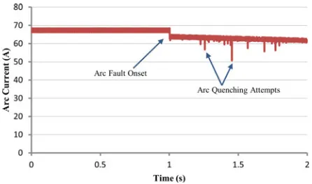
Fig. 1. Example of a sustained series arc current waveform.
through ionized gas during fault events may be fully sustained; the high heat generated can lead to partial volatilization of the conductors and increases the risk of fire to surrounding insula-tion [13]. There are many condiinsula-tions that may cause an arc fault, including [7] the following:
1) Chemical, electrical, and mechanical deterioration of wiring and interconnections.
2) Presence of moisture or fluids on the insulation enabling leakage currents to create small electrical discharges across voids to other conductors: this condition is termed
wet arc tracking.
3) Loose terminal connections.
Arc faults are categorized as either parallel or series—this paper focuses solely on the detection and diagnosis of series arc fault conditions. Series arcing usually begins with either chemi-cal corrosion of pin-socket connections or loose connections in series with loads. A significant detection issue with the series arc fault is the fact that, as the ionized gap is in series with the load, fault current actually decreases below load rated current and well below relay trip curves.
In dc-supplied systems there is no natural current zero. As a result, arcing conditions are more sustainable and, potentially, more dangerous—a typical series arc current waveform in a dc system is illustrated inFig. 1, where arcing over a sustained period is evident. This waveform was captured using a network model of a 270 Vdc rectifier interfaced system supplying a purely resistive load–the fault model described in Section IV-A was implemented in this network model to characterize the arc fault conditions. The hazards that series dc arc fault events pose to safety and reliability of supply, combined with the associated detection difficulties, have resulted in significant scope for the development of accurate diagnostic systems to mitigate their impact.
Systems for diagnosing arc faults are classified as either me-chanical or electrical [14]. Electrical-based systems extract arc features in the time [15], frequency [16], or time–frequency [17] domains, and algorithms analyze these extracted features to determine the presence of arcing events. The transient, nonsta-tionary characteristics of arcing conditions means that systems that rely on time–frequency domain extractions hold the most promise for accurate diagnosis of arc fault conditions.
Series dc AFD systems based on all three feature extraction methods have been proposed in the literature. Guo et al. [18] de-fined a system that identifies a period of time between a sudden
drop in load current and arc ignition as an arc precursor time. Kilroy et al. [19] developed a system based on averaging load current signals over time periods. Momoh and Button [20] pro-posed a system that used spectral energy from nominal and fault events to train separate artificial neural networks (ANNs). Other time-domain and frequency-domain series dc AFD methods are outlined in [21]–[23]. Yunmei et al. [24] described a system based on time–frequency domain features that utilized the en-ergy of extracted wavelet transform (WT) [25] coefficients for fault diagnosis. Yao et al. [26] developed a system based on time and time–frequency features for application to representative dc microgrid networks. The system used statistics calculated from current data, and coefficients extracted using the WT, for fault diagnosis.
Despite the development of multiple AFD systems, major challenges still exist concerning maintaining high diagnostic accuracy across a range of operating conditions. Accurately diagnosing faults that are often highly intermittent and cause re-ductions in system current is already a difficult task—attempting to develop an accurate and generalized diagnostic system is a significant challenge. Reliance on algorithms that compare ex-tracted features with basic thresholds, as the majority of these systems do, will not suffice in meeting this challenge based on robustness to noise alone. Consequently, this paper proposes IntelArc, a machine learning (ML) based system that uses ex-tracted features to train HMM and increases the potential for an accurate and generalized diagnostic performance.
III. HMM-BASEDARCFAULTDIAGNOSIS
A range of ML techniques have the potential to diagnose se-ries dc arc faults, including ANN [20], support vector machines (SVM) [27], and Bayesian networks [28]. HMMs [11] can be used in classification problems associated with noisy time-series data even though they do not have exact domain knowledge of the problem [29]. Traditional applications of HMM are in speech, handwriting, and gesture recognition [30]. More re-cently, they have been applied in classifying patterns in process trend analysis [31], machine condition monitoring [29], and ac transmission/distribution networks [32], [33]—they have not previously been applied for diagnosis of series dc arc faults. HMMs assume that the system modeled is a Markov process with unobserved (hidden) states and that system data is a noisy observation of this process.
Fig. 2. Outline of IntelArc method—only three trained HMM are illustrated for brevity: these relate to models of nominal steady-state, nominal transient, and series arc fault conditions, respectively. In practice, further HMM relating to different conditions could be trained and implemented within the framework.
attractive from the perspective of combining models, which can be performed through well-understood axioms of probabilistic inference. An HMM-based system is also highly scalable and can be readily updated (i.e., without retraining multiple models) to include models of emergent system conditions. Through for-mal model selection procedures, over-fitting of HMMs can be avoided — although choice of the most likely model could be undertaken by optimizing LL, using Bayesian information crite-rion (BIC) [30] instead ensures the fit is not overly representative of the training examples by penalizing model complexity.
IV. INTELARC—METHODOVERVIEW
Fig. 2outlines the method of the proposed IntelArc system. The system utilizes a framework of trained HMM relating to different network conditions. Features are extracted from win-dows of network current data and applied to each trained HMM within the framework for inference of series arc faults. Current can be sampled at various locations throughout the network and each load current window covers 50 ms of system operation. Each HMM outputs an LL measure, which quantifies the sim-ilarity of online data with the trained parameters of the HMM. An algorithm analyses the LL output of each HMM every 50 ms, and the system outputs an alarm if there is sufficient evidence to suggest the presence of arc fault conditions—50 ms was deemed a sufficient length of time to safely diagnose and isolate arcing conditions and also decrease the probability of false detections. The process is repeated as new windows of current data become available.
A. Generation of Arc Fault Data
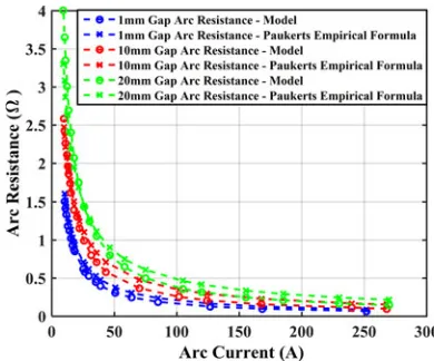
A software model was used for generation of arc fault data. The model was proposed by Uriarte et al.—a complete descrip-tion of the model is provided in [34]. The model was designed to represent arcing conditions between electrodes that separate at a constant speed and eventually dwell at a fixed distance. Arc voltage, current, and resistance outputs were compared to similar dc arc models within literature [35] to assess similarity and, thus, ensure that it is accurately representative of series dc arc conditions.
Fig. 3. Comparison of model outputs with Paukert’s formulas.
The model is a hyperbolic approximation of dynamic arc voltage and current that assumes arc impedance is predom-inantly resistive. Nonintermittent fluctuations in voltage and current are used to represent unsuccessful quenching attempts. Arc voltage gradient of the model, i.e., how voltage varies with arc gap, was compared with previously defined values by both Browne (12 V/cm) [36] and Strom (13.4 V/cm) [35].
Average gradient of the model wasࣈ10 V/cm. Despite ex-hibiting slightly lower values, there is agreement with Browne and Strom’s models, particularly for smaller electrode gaps. V−I
characteristics of fixed length arcs are generally considered to be inverse and nonlinear below a current transition level. For arc currents above this level (which is defined to be in the region of 10–13 A for small electrode gaps [37]), voltage increases only minimally with current. Evaluation of V–I model behavior showed minimal agreement with lower current characteristics, although it did accurately characterize voltage for current ranges above the transition level. In this sense, an associated caveat of the model is that voltage output at arc currents belowࣈ10A are less accurate.
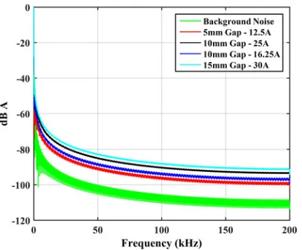
Fig. 4. Frequency spectrums throughout different arc fault conditions.
model where resistance increases significantly at lower current values and becomes almost constant at higher current. There is also acceptable agreement with Stokes, albeit with arc resis-tance slightly lower for corresponding current magnitudes—this suggests that arc voltage magnitude is slightly lower than the empirical formula proposed.
Arcing current frequency spectrums up to 200 kHz were ob-served within data simulated in the basic system model de-scribed in the following section using the fast Fourier transform (FFT)—spectrums across different fault conditions are illus-trated inFig. 4. Analysis of the spectrums highlighted greater energy content at higher harmonic levels under arcing condi-tions in comparison to nominal background noise. Indeed, there is roughly a 25 dB disparity at a frequency as low as 10 kHz. FFT results were comparable to those presented in [39].
Overall, these comparisons validate accuracy of the fault model with a sole inconsistency concerning V–I character-istics at low current levels. However, voltage gradients, arc impedance, and frequency characteristics showed relative agree-ment. Generation of intermittent series fault data was required to test IntelArc’s ability to accurately diagnose intermittent events. Hence, the sustained fault model proposed in [34] was extended to include fault intermittency. This extension includes func-tionality that randomly switches the voltage developed across a sustained arc fault from arc voltage to zero to represent in-termittent separation of contactors—the process of initiating a sustained fault and then switching voltage across the fault to zero at a random time after fault onset can be reproduced multi-ple times throughout one simulation run of the model to create intermittent conditions.
B. Arc Fault Feature Extraction and Selection
[image:4.594.56.275.64.245.2]In ML-based diagnostic systems, features extracted from data should be optimally discriminative between the different conditions/behaviors under consideration [40]. Extracting features in the time–frequency domain highlights the frequency components that are present at particular points of time in a signal—the transient characteristics of arc faults means that,
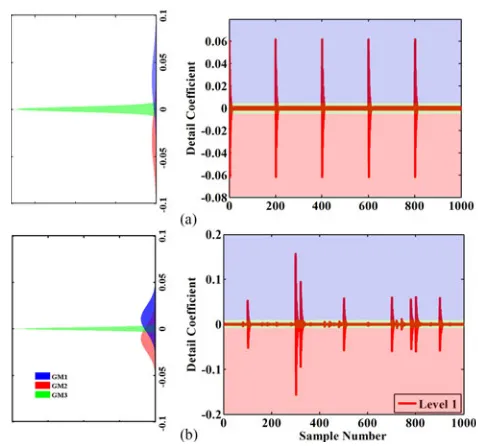
Fig. 5. Examples of dc current and associated DWT extractions for (a) nominal conditions and (b) arc fault conditions.
theoretically, there should be relatively significant differences between the time–frequency extracted features of nominal and fault conditions. The discrete WT (DWT) extracts different bands of frequencies from a signal through successive filtering and down-sampling. Different bands of high frequencies are output as detail coefficient levels, whereas bands of low frequen-cies are output as approximate coefficient levels [41]. Analyzing how the detail and approximate coefficient levels vary through-out different system conditions was the main goal of feature selection. For further information on DWT theory, refer to [41]. Training data were simulated using a basic system model comprising a six-pulse passive diode rectifier feeding an either purely resistive or reactive load. AC input to the rectifier was 230 Vac, with frequency varying between 50 and 400 Hz throughout different simulation runs, to provide 270 Vdc to the load. Fault conditions were initiated on the load feeder using randomized instances of the intermittent arc model described and validated in the previous section: speed of electrode separa-tion was randomized between 5 and 25 mm/s, and the distance at which the electrodes dwell was randomized between 1 and 15 mm. System current is sampled at 20 kHz and has 5 kHz noise—the noise model is Gaussian distributed with 0 mean and 0.001 variance that is sampled every 20 ms throughout each simulation to model sensor noise. Five kilohertz was chosen as this lies in the middle of the observed 0–10 kHz bandwidth of a 20 kHz sampled signal. The following sections describe feature extraction and selection from the simulated training data.
Fig. 6. Model of the DWT approximate extractions using a GMM for (a) nominal conditions and (b) arc fault conditions.
time–frequency response across the lower frequency subbands, and high-frequency noise is filtered out as the levels increase and subbands get both lower and narrower. In contrast,Fig. 5(b) shows an example of normalized current data during arc fault conditions with associated extracted approximate coefficients. The sudden decrease in load current is a result of an unsuccess-ful quenching attempt that, in comparison toFig. 5(a), signif-icantly changes the magnitude and shape of the approximate coefficients during fault conditions.
Diagnostic systems based on HMM rely on features that cture temporal dynamics—modeling the distribution of the ap-proximate coefficients using a Gaussian mixture model (GMM) [30] enables the dynamics of each coefficient to be assessed through designation of each data sample to a particular mixture. As an example, GMMs of approximate level 1 coefficients were developed using the nominal and series arc fault training data to analyze the dynamics across each condition and determine features that increase discrimination capabilities, as illustrated inFig. 6(a)and(b), respectively. The following steps were un-dertaken throughout GMM development:
1) Analysis of the distribution of DWT coefficients for each condition—a nonparametric Kernel density estimation was used to determine general shape of the distribution. 2) Use of Gaussian distributions to analyze the probability of
coefficients falling between specified ranges in the data— the example inFig. 6shows four different Gaussians that model the distribution of four different ranges in the data, although this number may vary depending on desired resolution.
Within the fault condition GMM there is significant disparity between the areas of each Gaussian mixture with an increased probability of coefficients exhibiting magnitudes close to 1. In comparison to nominal conditions, the number of transitions between mixtures across a sequence of data samples is likely
Fig. 7. Model of the DWT detail extractions using a GMM for (a) nominal conditions and (b) arc fault conditions.
to be significantly less. These differing characteristics high-lighted that approximate coefficients are a useful feature for discriminating between nominal and series arc fault conditions. Selecting the levels of coefficients was necessary to optimize detection accuracy and limit feature redundancy. It was evident from analysis of the extracted DWT approximations that coeffi-cients begin to level out as the levels increase and the frequency subbands get closer to zero—the examples inFig. 5emphasize the flatness of level 5 coefficients in comparison to levels 1 and 3. This is not ideal as the distributions begin to cluster within cer-tain regions, and this reduces the number of transitions during nominal conditions. Consequently, DWT approximate coeffi-cient levels 1, 2, and 3 were selected as suitable features for AFD to minimize the effect of extremely low-frequency bands on detection accuracy.
2) Time–Frequency Domain Extraction—Detail Coeffi-cients: Transient arc fault signals contain high-frequency com-ponents that are also potentially useful for detection. The DWT detail coefficients, which extract high-frequency components, are therefore an important feature to consider. Similar to the case of approximate coefficients, it is necessary to select detail coefficients that optimally discriminate between various condi-tions.
Fig. 7illustrates GMMs of detail level 1 coefficients for both nominal and fault conditions extracted from 50 ms windows of normalized current data during each condition. Current dur-ing nominal conditions contains both dc ripple and measurement noise; dc ripple results in levels 1 and 3 coefficients increase ev-ery 12.5 ms (or 200 samples for a 20 kHz sampled signal). Measurement noise also increases the magnitude of detail coef-ficients; however, as noise is random, the coefficient increases are less predictable. Five kilohertz noise has a notable effect on level 3, whereas there is less effect on level 1.
[image:5.594.44.291.64.291.2]particularly evident at the lower levels—relative to nominal sys-tem conditions, coefficient magnitude increases at lower levels are significantly more prominent under fault conditions. The increased probability of higher coefficient magnitudes results in a greater number of transitions between mixture components in a GMM of fault conditions—in comparison, the GMM of nom-inal condition data has significantly less transitions between mixtures. The differences in detail coefficients between condi-tions confirm that they are an excellent feature for use in the HMM-based IntelArc. Analysis of each detail level showed that levels 3–5 did not optimize discrimination between each con-dition as they do not capture the higher frequency transients present throughout the arc fault events.
In practice, noise from power electronic converters will not be limited to 5 kHz and may be present across the entire 0−10 kHz observable bandwidth. Noise between 5 and 10 kHz will have an effect on lower level detail extractions; however, the salient higher frequency signatures of arcing will still be present within these features, and they will remain useful for diagnosis. This is not the case at increased detail levels as the higher frequency components are filtered out–their inclusion in IntelArc will likely impair detection. Consequently, the number of DWT detail extractions is limited to lower levels, with only levels 1 and 2 being selected as suitable features.
3) Summary of Arc Fault Feature Extraction and Se-lection: The process of modeling the probability distributions of extracted coefficients under different network conditions is critical for using HMM for AFD as it enables appreciation of the coefficient dynamics under each network condition and sim-plifies the HMM training stage. While previously proposed sys-tems [26] have used WT extracted features for AFD, the studies outlined here, to the best of knowledge, are not available in literature.
The author’s studies determined that the three approximate and two detail DWT coefficients extracted from system current with a 20-kHz sampling frequency would be utilized for series dc arc fault detection within the IntelArc system.
Time-domain features were also extracted using statisti-cal analysis of the windows of system current data. Specifi-cally, a time-domain feature based on a moving average across 50-ms windows was extracted. Calculation of the moving av-erage limits dc ripple and separates the normalized data into distinct regions for each condition. Signals are also generally smoother, with the majority of high-frequency noise removed. The feature is complementary to the WT coefficients as the general distinctions between nominal and fault conditions are highlighted.
C. HMM Training
Feature selection determined that in total six feature vectors were used to train each HMM. These features included:
1) DWT approximation coefficient levels 1, 2, and 3; 2) DWT detail coefficient levels 1 and 2;
3) moving average of system current.
The number of hidden states and mixture components for each HMM within the system are summarized inTable I. The
TABLE I
NUMBER OFHIDDENSTATES ANDMIXTURESWITHINEACHHMM
HMM Model No. of Hidden States No. of Mixtures
Nominal steady state 10 10 Nominal transient 4 4 Series dc arc fault 6 6
increased number of hidden states in the nominal steady-state model is a consequence of the WT approximation features as a greater number of states emphasize higher transition rates. Lim-iting the number of hidden states and mixture components of the fault and nominal transient models reduces the risk of over-fitting the models to training examples; overover-fitting the nominal steady-state model is less of an issue as data under this condition is likely to be more consistent across a range of network sce-narios. The expectation–maximization algorithm [30] was used for model training.
D. AFD Algorithm
Accurate AFD within IntelArc is dependent on correct inter-pretation of the LL outputs of each trained HMM—this section provides examples of these outputs throughout various network conditions and describes the algorithm for analyzing them to in-fer network condition. Online application of IntelArc involves the use of features extracted from 50 ms windows of current data being recursively applied to each trained HMM. Sliding win-dows with an interval of 10 ms and overlap of 40 ms are applied to the fault and nominal HMM, while 50 ms consecutive win-dows are applied to the nominal transient HMM. The algorithm analyses the LL outputs of each HMM at 50 ms intervals— hence, five LL outputs from the nominal and fault models and one LL output from the nominal transient HMM are analyzed at each interval. The use of sliding windows is advantageous for detection of intermittent arc events as there is increased poten-tial for detection of changes in fault current across shorter time frames.
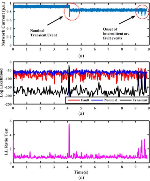
Fig. 8(a)illustrates a typical example of dc network current across steady-state, nominal transient and intermittent series arc fault conditions: a simple load switch models a nominal transient event and is evident at roughly 4 s while intermittent arcing events develop at roughly 9 s and results in periods of a decreased system current. Both the duration of each intermittent fault event and the level of current reduction are variable, and the aim of the system is to diagnose these highly variable events in real-time. The corresponding LL outputs of each trained HMM are illustrated inFig. 8(b). The only points in time throughout the 10-s period where the LL of the nominal model is not greater than both the fault and transient model LLs are during the load switching event and the intermittent arcing events.
Fig. 8. (a) Example of network current throughout various conditions, (b) corresponding LL outputs of trained HMM, and (c) LL ratio test. Note the increase at 4 s caused by the nominal transient event—the corresponding LL increase of the transient model beyond the nominal and fault models at this point results in no fault being diagnosed.
the LL of the fault model increases beyond that of the nominal and transient models, which is indicative that arc fault condi-tions are present, and hence, diagnosis of a fault is prescribed by the system.
Another useful measure used that indicates an increased prob-ability of fault presence is an LL ratio test [30] between the nominal and fault models—this ratio quantifies the difference between the two hypotheses, and points in time where it is greater than 1 may imply series arc fault conditions. An il-lustration of the LL ratio test for this example is provided in Fig. 8(c).
A summary of the complete IntelArc method, including appli-cation of network data to each trained HMM and the algorithm for interpretation of the model outputs, is illustrated inFig. 9. The algorithm compares the LL outputs to predetermined thresh-olds to determine if there is a significant probability of series arc fault presence during each 50 ms observational period. If all of the specifications described inFig. 9 are not met, nominal operation is assumed.
Predetermined thresholds were set through analysis of HMM LL outputs across different operational scenarios. Normaliza-tion ensures IntelArc is generally neutral to different levels of dc ripple and current magnitude. However, performance may be affected by different forms of reactive loading. Dif-ferences in inductive and capacitive loading may impact set-ting of LL thresholds, and it is therefore imperative that
di-Fig. 9. Summary of the complete IntelArc method.
agnostic performance is assessed across different types of load—the case studies in the following section investigates these issues.
V. CASESTUDIES
The two case studies described in this section were used to evaluate and validate diagnostic accuracy of IntelArc. The basis of the first case study is the repeated injection of intermittent series arc faults into a dc power network model for generation of test data where the time of fault onset (s) is known; the test data is input to the system for inference of network condition, and its outputs are compared with known behavior to verify accuracy and detection time. The second case study used fault data generated using a representative dc testbed to test IntelArc accuracy.
A. Case Study 1: DC Network Model and Testing Methodology
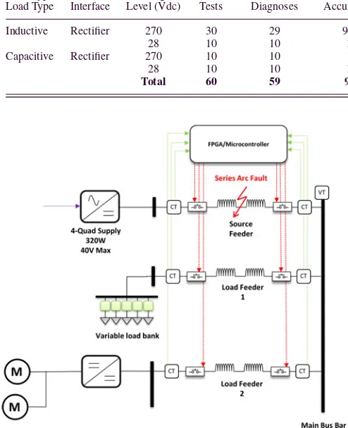
[image:7.594.46.288.64.355.2]Fig. 10. Test dc network model architecture.
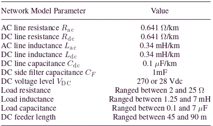
two load centers through separate feeders. This basic network architecture may be representative of low-voltage dc microgrids that are either interconnected with a main grid [1] or stand-alone, e.g., within an aircraft or shipboard system [2], [43]. The passive rectifier has either 230 Vac input to commutate to 270 Vdc or 115 Vac input to commutate to 28 Vdc—these are typical distribution levels in aerospace applications. Lumped element models consisting of resistors, inductors and capacitors were used to model resistive and reactive loads. The two load centers are directly interfaced to the system and do not include addi-tional conversion stages. Series arc faults were modeled on the load feeders and current through the feeder is sampled at either the load centers or the bus bar. Practically, it would be more suitable for current to be sampled at the main distribution bus bar to relieve hardware issues—measurements would be com-municated to a central data acquisition system for processing, which, in turn, would communicate to protection devices in the event of fault detection. As part of the case study, a total of 60 model simulations were run for generation of individual test cases, where each simulation lasted 10 s. Each test case includes periods of nominal steady-state behavior on both load feeders, nominal transient events on both feeders, and series intermittent arc fault behavior on one feeder. The current profile inFig. 8(a) is a typical example of simulated current on the faulted feeder throughout one of the test cases. Nominal transient events are modeled through basic switching of loads within the load cen-ters. To fully test the generalization capabilities of IntelArc, network parameters such as feeder lengths, fault location along the feeder, onset and duration of each fault event, load types, and voltage levels were varied throughout each simulation run, and 5 kHz Gaussian noise was added to the sampled current to model sensor noise—a description of the network model parameters is provided inTable II. Forty tests were conducted at 270 Vdc, and 20 were conducted at 28 Vdc. This case study does not con-sider switching noise from active power converters. Each 10-s test case was divided accordingly into individual data windows
TABLE II
TESTDC NETWORKMODELPARAMETERS
Network Model Parameter Value
AC line resistanceRa c 0.641Ω/km
DC line resistanceRd c 0.641Ω/km
AC line inductanceLa c 0.34 mH/km
DC line inductanceLd c 0.34 mH/km
DC line capacitanceCd c 0.1µF/km DC side filter capacitanceCF 1mF DC voltage levelVD C 270 or 28 Vdc
Load resistance Ranged between 2 and 25Ω Load inductance Ranged between 1.25 and 7 mH Load capacitance Ranged between 0.1 and 7µF DC feeder length Ranged between 45 and 90 m
and applied sequentially to the AFD system, as described in Section IV-D.
1) Case Study 1: Results: Results of the 60 individual test cases are summarized in Table III. In total, 59 out of 60 test cases were correctly diagnosed equating to overall accu-racy of 98.3% and an average detection time from fault onset of 57.1 ms: the incorrectly diagnosed test case was the result of a false positive (FP) during a nominal transient event under induc-tive loading. 97.5% of 270 Vdc tests were accurately diagnosed while 100% of the arcing events at 28 Vdc were accurately iden-tified. This basic case study has highlighted various attributes of the proposed system, including the following:
1) detection of variable duration intermittent arcing events; 2) detection of arcing events with variable decreases in load
current magnitude;
3) detection across a range of load currents; 4) accurate detection of all intermittent fault events; 5) some instances of nominal system transients result in
false detection;
6) acceptable detection time.
Original testing highlighted a higher rate of FPs as a result of nominal transients. This was attributed to the LL of the nominal steady-state model significantly decreasing at the transient event (as expected) before increasing to a value more associated with fault conditions immediately after the switching event, which results in the system incorrectly diagnosing the presence of an arc fault. To alleviate this problem, it was determined that diag-nosis of a fault event cannot be made for 100 ms after a transient event has been diagnosed. Traoffs do exist between false de-tection, nondede-tection, and detection time. LL thresholds may be tuned to improve issues surrounding the rate of FPs although this may lead to nondetection of some intermittent events (there was no occurrence of false negatives in the test cases) as well as an increased detection time. Future work will continue to optimize thresholds to improve accuracy and refine reliability of the method to move towards commercial application.
Fig. 11. One-line diagram of dc testbed setup.
Fig. 12. (a) Depiction of various components within the experimental dc testbed configuration and (b) series arc fault throwing unit.
A similar line of discussion extends to the type of load interface whereby the internal control of power electronic converters can also alter fault current dynamics [44].
B. Case Study 2
The IntelArc method has also been tested using data gener-ated within a dc network testbed, which has means of inducing series arc faults. These initial experimental studies have tested the methods ability to accurately diagnose faults in the pres-ence of converter and measurement noise. A one-line diagram
of the testbed is illustrated inFig. 11and photographs depicting various system elements are provided inFig. 12. The setup con-sists of a four-quad active rectifier providing dc power to a main bus bar through two solid-state power controllers (SSPCs). Two separate loads, a directly interfaced resistive load bank, and two parallel motors interfaced using a buck–boost dc/dc converter are connected to the main bus bar. Two current measurements are taken at each respective feeder, and a voltage measurement is taken at the main bus bar. This equipment and configuration is limited to a maximum of 40 V, 320 W, which allows representa-tion of low-voltage dc networks. As part of the case study, series arc faults were induced between the source and the bus bar with use of a fault throwing unit that consists of a stepper motor in-termittently separating two contacts [34][seeFig. 12(b)]. Also, switching within the variable load bank was used to capture nominal transient behavior. Electrical current data sampled at 20 kHz was captured at the source feeder using an oscilloscope during steady state, series arc fault and nominal load switching behaviors. This data were used to test the accuracy of the In-telArc method that was trained using data generated from the software model described in Section IV.
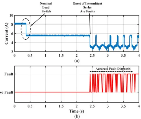
Current data captured at the source feeder and the cor-responding diagnostic outputs of IntelArc are illustrated in Fig. 13. Within this test example, the nominal load switch did not result in false diagnosis, while the intermittent fault condi-tions were accurately diagnosed. Five tests have been conducted with the onset of arcing occurring at two different power levels outlined inTable IV—IntelArc accurately identified the onset of fault conditions in each test case and load switching behavior did not result in FPs.
The next significant step would be implementing IntelArc onto the microcontroller. Testbed data would be collected, pro-cessed and analyzed using the integrated microcontroller to al-low diagnosis of series arc faults in real time. In the event of fault detection, control signals would be communicated to SSPCs to isolate the fault and thus test time between fault onset and isolation.
C. Comparison of IntelArc With Existing AFD Methods
[image:9.594.45.289.451.576.2]Fig. 13. (a) Experimental data captured using the dc testbed. Within this test case, a nominal load switch occurred at 0.4 s and the onset of intermittent series arcing occurred at 2.4 s. (b) Corresponding diagnostic outputs of the IntelArc. IntelArc is not affected by the nominal load switch and accurately detects arcing at the appropriate time.
TABLE IV
SUMMARY OFCASESTUDY2 RESULTS
Voltage Level (V) Current Level (A) No. of Tests IntelArc Accuracy (%)
33 5.5 3 100
28 8 2 100
highlighted the ability of IntelArc to detect accurately across 270 and 28 Vdc levels and different forms of reactive loading. The detection time is in the order of 100 ms—almost double the average detection time of IntelArc. Test results of the ANN method utilizing FFT features in [20] showed limited accuracy in fault cases in comparison to IntelArc, as only 40% of 5 fault scenarios were accurately diagnosed. Testing did not consider nominal transient behavior. The main limitation of frequency domain extractions of nonstationary transient arc fault signals is there is no representation of how the frequency contributions change throughout time.
The DWT analysis method in [24] claims high accuracy, although generalization is not proven as test results are only provided at 28 Vdc levels and values of load impedance are unchanged throughout testing. The method relies on observa-tion of a certain number of abnormal events over a 100 ms period—thus, minimal detection time will be 100 ms.
A benefit of HMMs is the minimal computation effort re-quired during calculation of LL statistics. IntelArc would be computationally inexpensive as only the trained parameters, and not associated training data, of each HMM are required for hard-ware implementation. The basis of the algorithm itself are the Viterbi algorithm [47] for calculating the LL of each HMM and the DWT for feature extraction—the Viterbi algorithm has com-putational complexity ofO(N2T), where T is the number of hidden states in each model, and the one-dimensional (1-D) db2
DWT has linear complexityO(N). The overall effect of com-putational complexity on fault detection time is an avenue for further investigation and will be assessed with further hardware implementation.
Overall, the IntelArc method, that combines DWT feature extractions with HMM, provides an excellent platform for ac-curate, generalized and robust diagnosis of series dc arc faults.
VI. CONCLUSION
This paper has proposed IntelArc, a series AFD system for application to dc networks, which is based on HMM and uti-lizes time–frequency and time-domain features extracted from network current data. The choice of advanced ML method was motivated by the need to improve diagnostic accuracy and gen-eralize across a range of network operating conditions. In par-ticular, analysis of the temporal dynamics of DWT coefficients and their use for implementation within the HMM-based sys-tem determined the ranges of detail and approximate coefficients that would optimize system performance. Two case studies val-idated accuracy of the method. IntelArc can now be further tested in the dc testbed with the benefit of using an accurate arc fault software model. In this context, development would remain software based with utilization of data from the validated arc fault model to train the respective fault HMM; parameters and algorithms would be integrated onto a microcontroller and the methods ability to isolate faults would be tested in real-time. Ac-celerating IntelArc through technology readiness levels (TRL) will require further consideration of the effect that noise emis-sions and interference from system devices have on detection accuracy. Deployment within compact dc networks, with cur-rent sensors located at the closest upstream bus bar, means that transmitted fault signals and data should remain uncorrupted. However, further consideration will also be given to this issue at higher TRL.
The aspect of software development for hardware application would be of significant importance and benefit; while the abil-ity of ML approaches for various forms of fault diagnosis are well documented [45], the main drawback of their approach is a requirement for fault data, which is often unavailable. Access to an accurate series arc fault model that enables instances of fault data to be readily available, and from which a generalized, accurate AFD system could be developed, is of significant ad-vantage. The adoption of dc distribution is prevailing, and this paper has shown the potential for IntelArc to improve reliability and security of supply within such networks through diagnosis and isolation of hazardous and difficult-to-detect series arc fault conditions.
REFERENCES
[1] D. Salomonsson et al., “Protection of low-voltage DC microgrids,” IEEE Trans. Power Del., vol. 24, no. 3, pp. 1045–1053, Jul. 2009.
[2] S. D. A. Fletcher et al., “Determination of protection system require-ments for DC unmanned aerial vehicle electrical power networks for enhanced capability and survivability,” IET Electr. Syst. Transp., vol. 1, no. 4, pp. 137–147, Dec. 2011.
Conf., Austin, TX, USA, Jun. 2012, pp. 1–5.
[9] M. Faifer et al., “A method for the detection of series arc faults in DC aircraft power networks,” in Proc. IEEE Instrum. Meas. Technol. Conf., Minneapolis, MN, USA, May 2013, pp. 778–783.
[10] J. D. Herbst et al., “Flexible test bed for MVDC and HFAC electric ship power system architectures for navy ships,” in Proc. IEEE Electric Ships Technol. Symp., Alexandria, VA, USA, Apr. 2011, pp. 66–71.
[11] L. R. Rabiner, “A tutorial on hidden Markov models and selected appli-cations in speech recognition,” Proc. IEEE, vol. 77, no. 2, pp. 257–286, Feb. 1989.
[12] V. V. Terzija and H. J. Koglin, “On the modelling of long arc in still air and arc resistance calculation,” IEEE Trans. Power Del., vol. 19, no. 3, pp. 1012–1017, Jul. 2004.
[13] D. Li et al., “A method for residential series arc fault detection and iden-tification,” in Proc. IEEE Conf. Electr. Contacts, Vancouver, BC, Canada, Sep. 2009, pp. 8–14.
[14] G. Liu et al., “A survey on arc fault detection and wire fault location for aircraft wiring systems,” SAE Int. Jour. Aerosp., vol. 1, no. 1, pp. 903–914, Jan. 2008.
[15] J. C. Zeurcher and D. L. McClanahan, “Apparatus and method for real time determination of arc fault energy, location and type,” U.S. Patent 7 068 045, Jun. 27, 2006.
[16] M. T. Parker et al., “Electric arc monitoring systems,” U.S. Patent 6 772 0777, Aug. 3, 2004.
[17] M. Michalik et al., “High impedance fault detection in distribution net-works with use of wavelet based algorithm,” IEEE Trans. Power Del., vol. 21, no. 4, pp. 1793–1802, Oct. 2006.
[18] S. Y. Guo et al., “DC arc detection and prevention circuit and method,” U.S. Patent 6 683 766, Jan. 27, 2004.
[19] D. G. Kilroy and W. H. Oldenburg, “DC arc fault detection and protection,” U.S. Patent 2007/0 133 135, Dec. 5, 2006.
[20] J. A. Momoh and R. Button, “Design and analysis of aerospace dc arcing faults using fast Fourier transformation and artificial neural network,” in Proc. IEEE Power Eng. and Soc. General Meeting, Toronto, ON, Canada, 2003, pp. 788–793.
[21] M. Dargatz and M. Fornage, “Method and apparatus for detection and control of dc arc faults,” U.S. Patent 8 179 147, May 15, 2012. [22] J. Zeurcher et al., “Detection of arcing in dc electrical systems,” U.S.
Patent 2004/0 027 749, Feb. 12, 2004.
[23] Y. Ohta and H. Isoda, “Arc detecting device and aircraft equipped there-with,” E.U. Patent 2 120 306, Nov. 18, 2009.
[24] G. Yunmei et al., “Wavelet packet analysis applied in detection of low voltage dc arc fault,” in Proc. IEEE Conf. Ind. Electron. Appl., Xi’an, China, 2009, pp. 4013–4016.
[25] The wavelet tutorial. (1999).[Online]. Available: http://person.hst.aau.dk/ enk/ST8/wavelet_tutotial.pdf. Accessed on: Jul. 16, 2015.
[26] X. Yao et al., “Characteristic study and time-domain discrete wavelet transform based hybrid detection of series DC arc fault,” IEEE Trans. Power Electron., vol. 29, no. 6, pp. 3103–3115, Jun. 2014.
[27] M. Sarlak and S. M. Shahtrash, “SVM based method for high impedance fault detection in distribution networks,” Int. J. Comp. Math. Electr. Elec-tron. Eng., vol. 30, no. 2, pp. 431–450, 2011.
[28] O. J. Mengshoel et al., “Probabilistic model-based diagnosis: An electrical power system case study,” IEEE Trans. Syst., Man, Cybern. A., Syst., Humans, vol. 40, no. 5, pp. 874–885, Sep. 2010.
[29] Q. Miao and V. Makis, “Condition monitoring and classification of rotating machinery using wavelets and hidden Markov models,” Mech. Syst. Signal Process., vol. 21, no. 2, pp. 840–855, Feb. 2007.
[30] K. P. Murphy, Machine Learning: A Probabilistic Perspective. Cambridge, MA, USA: MIT Press, 2012.
vol. 102, no. 1, pp. 27–37, 1955.
[37] A. D. Stokes and W. T. Oppenlander, “Electric arcs in open air,” J. Phys. D: Appl. Phys., vol. 24, no. 1, pp. 26–35, Jan. 1991.
[38] J. Paukert, “The arc voltage and arc resistance of LV fault arcs,” in Proc. Int. Switching Arc Phenomenon Symp., Lodz, Poland, 1993, pp. 1–4. [39] J. Johnson and K. Armijo, “Parametric study of PV arc-fault generation
methods and analysis of conducted DC spectrum,” in IEEE Photovoltaic Specialist Conf., Denver, CO, USA, Jun. 2014, pp. 3543–3548. [40] S. Khalid et al., “A survey of feature selection and extraction techniques in
machine learning,” in Proc. Sci. Inform. Conf., London, U.K., Aug. 2014, pp. 372–378.
[41] R. X. Gao and R. Yan, “From Fourier transform to wavelet transform: A historical perspective,” in Wavelets: Theory and Applications for Manu-facturing. Springer Science, Berlin, Germany, 2011, ch. 2, pp. 17–32. [42] Wavelet Toolbox. [Online]. Available: http://uk.mathworks.com/
products/wavelet/. Accessed: 03-Feb-2016.
[43] X. Feng et al., “Multi-agent system based real time fault management for all-electric ship power systems in DC zone level,” IEEE Trans. Power Syst., vol. 27, no. 4, pp. 1719–1728, Nov. 2012.
[44] Codes and Standards for PV Arc Fault Mitigation. (2010).[Online]. Avail-able: http://energy.sandia.gov/wp-content/gallery/uploads/Bower_Arc-PV_Codes-Detection-mitigation.pdf. Accessed on: Feb. 04, 2016. [45] W. G. Fenton et al., “Fault diagnosis of electronic systems using intelligent
techniques: A review,” IEEE Trans. Syst., Man, Cybern. C, Appl. Rev., vol. 31, no. 3, pp. 269–281, Aug. 2001.
[46] Z. Wang et al., “Arc fault signal detection—Fourier transformation vs. wavelet decomposition techniques using synthesized data,” in Proc. Pho-tovoltaic Specialist Conf., Denver, CO, USA, 2014, pp. 3239–3244. [47] G. D. Forney, Jr., “The Viterbi algorithm,” Proc. IEEE, vol. 61, no. 3,
pp. 268–278, Mar. 1973.
[48] Simscape Power Systems. (2016). [Online]. Available: http://uk. mathworks.com/products/simpower/. Accessed on: Sep. 20, 2016.
Rory David Telford received the B.Eng. and M.Sc. degrees in electronic and electrical engi-neering in 2008 and 2011, respectively, from the University of Strathclyde, Glasgow, U.K., where he is currently working toward the Ph.D. degree in electronic and electrical engineering.
He is currently a Research Assistant within the Institute for Energy and Environment, Uni-versity of Strathclyde. His current research interests include application of AI techniques, data-driven fault diagnostics, and power system modeling and analysis.
Stuart Gallowayreceived the M.Sc. and Ph.D. degrees in mathematics from the University of Edinburgh, Edinburgh, U.K., in 1994 and 1998, respectively.
Bruce Stephen (M’09–SM’14) received the B.Sc. degree from Glasgow University, Glasgow, U.K., in 1997 and the M.Sc. and Ph.D. degrees from the University of Strathclyde, Glasgow, in 1998 and 2005, respectively.
He is currently a Senior Research Fellow with the Institute for Energy and Environment, Uni-versity of Strathclyde. His current research in-terests include power system condition monitor-ing, renewable integration, and characterization of low-voltage network behavior.
Ian Eldersreceived the B.Eng. degree (Hons.) and the Ph.D. degree from the University of Strathclyde, Glasgow, U.K., in 1994 and 2002, respectively.