Trim influence on Kriso Container Ship (KCS) : an experimental and numerical study

Proceedings of the ASME 2017 35th International Conference on Ocean, Offshore and Arctic Engineering OMAE2017 June 25-30, 2017, Trondheim, Norway

OMAE2017-61860

TRIM INFLUENCE ON KRISO CONTAINER SHIP (KCS); AN EXPERIMENTAL AND

NUMERICAL STUDY

ABSTRACT

There has been a lot of interest in trim optimisation to reduce fuel consumption and emissions of ships. Many existing ships are designed for a single operational condition with the aim of producing low resistance at their design speed and draft with an even keel. Given that a ship will often sail outside this condition over its operational life and moreover some vessels such as LNG carriers return in ballast condition in one leg, the effect of trim on ships resistance will be significant. Ship trim optimization analysis has traditionally been done through towing tank testing. Computational techniques have become increasingly popular for design and optimization applications in all engineering disciplines. Computational Fluid Dynamics (CFD), is the fastest developing area in marine fluid dynamics as an alternative to model tests. High fidelity CFD methods are capable of modelling breaking waves which is especially crucial for trim optimisation studies where the bulbous bow partially emerges or the transom stern partially immerses. This paper presents a trim optimization study on the Kriso Container Ship (KCS) using computational fluid dynamics (CFD) in conjunction with towing tank tests. A series of resistance tests for various trim angles and speeds were conducted at 1:75 scale at design draft. CFD computations were carried out for the same conditions with the hull both fixed and free to sink and trim. Dynamic sinkage and trim add to the computational cost and thus slow the optimisation process. The results obtained from CFD simulations were in

good agreement with the experiments. After validating the applicability of the computational model, the same mesh, boundary conditions and solution techniques were used to obtain resistance values for different trim conditions at different Froude numbers. Both the fixed and free trim/sinkage models could predict the trend of resistance with variation of trim angles; however the fixed model failed to measure the absolute values as accurately as the free model. It was concluded that a fixed CFD model, although computationally faster and cheaper, can find the optimum trim angle but cannot predict the amount of savings with very high accuracy. Results concerning the performance of the vessel at different speeds and trim angles were analysed and optimum trim is suggested.

INTRODUCTION

It is well known that fuel costs are one of the biggest operational costs for ship operators and any reduction can have a significant impact on operational expenses. Fluctuating fuel prices have been driving ship owners and operators to be more efficient within the last decade. Low operational costs are essential to be competitive in such conditions. Fuel efficiency has become one of the key objectives in the shipping industry with the newly adopted mandatory measures to reduce emissions too. Hence, shipping companies find themselves obliged to take measures for increased efficiency – so as to continue to operate economically in spite of rising costs, and also to cope with more strict environmental regulations imposed by IMO.

Emil Shivachev University of Strathclyde Glasgow, United Kingdom

Mahdi Khorasanchi University of Strathclyde Glasgow, United Kingdom

Trim optimisation is one of the easiest and cheapest methods among many fuel-saving measures recommended by IMO as it does not require any hull shape modification or engine upgrade [1]. Research from various parties has found that by sailing under optimal trim conditions, vessels can reduce fuel consumption by 2-5%, with a corresponding reduction in greenhouse gas emissions [2][3]. Many classification societies and vessel monitoring system providers already offer trim optimisation services. Hence it is already an attractive measure for ship owners. According to a market survey study by HSH Nordbank [4], 71 percent of the survey participants are optimising the trim of their ships.

This paper presents a trim optimisation study based on experiments and numerical simulations in calm water for the wel-known benchmark Kriso Container Ship (KCS). These two methods are commonly used to predict ship resistance. Larsen et al [5] presented a comprehensive trim optimization study which includes analysis of resistance and propulsive origin factors by conducting model tests, high fidelity CFD and potential theory CFD. Iakovatos et al [6] investigated the influence of trim on resistance of five different hull models through calm water experiments and pointed out the importance of experimental investigation of vessels’ resistance performance to optimise vessels trim. Sun et al [7] developed a trim optimization program through use of CFD for resistance calculations and tested it on a real container ship to prove the benefits of trim optimization.

As proved by previous studies in literature it is crucial to predict resistance accurately and efficiently for trim optimisation. In the present study, or the initial development of trim optimisation the mean draft was kept constant at design draft of 10.8 m Experiments were carried out at different trim angles for a range of speeds between 18 knots to 24 knots. For the numerical trim optimisation study two different speed values are investigated. First the speed was fixed at design speed of 24 knots (Froude number 0.26) and later slow steaming speed of 19 knots (Froude number 0.20) was investigated at design draught (10.8 m) and ballast draught (9 m) conditions.

To assess the effect of ship motions on optimum trim numerical calculations were carried out for both ship fixed at rest position and dynamic sinkage and trim. Experiments were performed only for free sink and trim model. Consideration of sinkage and trim is important as dynamic sinkage and trim add to the computational cost and thus may slow the optimisation process.

EXPERIMENTAL INVESTIGATION

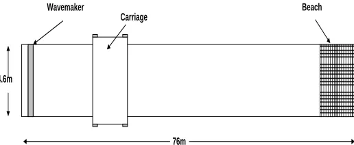
Experiments were carried out in the Kelvin Hydrodynamics Laboratory of the University of Strathclyde which has following specifications and features;

 Tank dimensions (LxWxD): 76m x 4.6m x 2.5m  Carriage: Driven along rails by a computer-controlled

digital driven DC motor. (Max speed 5m/s)

 Wavemaker: Variable water depth computer-controlled four-flap absorbing wavemaker. Capable of generating regular and irregular waves of up to approximately 0.5m

 Beach: At the opposite end of wavemaker there is a beach for the absorption of the waves and reducing reflection

4.6m

76m

Wavemaker Beach

Carriage

Figure 1 Kelvin Hydrodynamics laboratory

Description of the tested model

Table 1 Principal dimensions of the KCS model

Dimensions Full scale Model Scale

Scale 1.00 75

LPP (m) 230.0 3.0667

BWL (m) 32.2 0.4293

D (m) 19.0 0.2533

T (m) 10.8 0.144

Displacement (m3_{) 52030 0.1203}

S w/o rudder 9530 1.675

CB 0.651 0.651

CM 0.985 0.985

Test condition

T 10.8 0.144

Displacement (m3_{) 52030 0.1203}

S (m2) incl. rudder 9645 1.675

LCG 111.6 1.49

GM 0.60 0.097

Ixx/B 0.40 0.40

Izz/Lpp 0.25 0.25

Design speed

U (m/s, full scale: kn) 24 1.426 Fr (based on Lpp) 0.26 0.26

model tow point is located at the LCG of the vessel and at a vertical point relative to the shaft line.

All the tests were performed in fresh water and water temperature was recorded regularly during the tests. Model resistance, dynamic trim and sinkage, bow motions and actual speed of the model were recorded during the runs for calm water as shown in the table above. The model was only allowed to heave and pitch while other degrees of freedom were restricted.

Tests were carried out for a certain number of different trim angles at different speeds. Selected trim angle values range from 0.25 degree up to 1 degree for bow and stern trim conditions to ensure complete propeller immersion. These angles correspond to 1m to 4m trim in full scale.

Uncertainty analysis of the experiments was carried out by repeating the resistance tests 6 times at the same conditions at the velocity of Fr = 0.26 according to ITTC guides [8]. The standard uncertainty component of the mean from N repeat tests is estimated by

u'A(mean)=StDev / √N

where StDev is the standard deviation. It should be noted that the standard uncertainty of any single tests can be estimated by StDev or

u'A(single)= u'A(mean) * √N

Table 2 Uncertainty of repeat measurements for total resistance

Fr

RT (N) at (15.1°C)

Mean StDev u'A(mean) u'A(single) 2.u'A(single)

0.26 7.5073 0.49% 0.16% 0.49% 0.98%

It is shown from Table 2 above that resistance of this model is estimated at ±1.0% at 95% confidence level.

NUMERICAL INVESTIGATION

Numerical simulations were set up to investigate the effect of dynamic sinkage and trim. Commercial CFD software STAR-CCM+ was used and Reynolds Averaged Navier-Stokes (RANS) approach was adopted. Standard k-ε turbulence model was chosen following many other studies such as Enger et al [9] and Tezdogan et al [10]. Free surface was captured by VOF method.

Ship motions were restricted for the fixed case simulations and allowed for free case simulations in the pitch and heave directions. Dynamic Fluid Body Interaction (DFBI) model was employed for free cases in order to predict the realistic ship behaviour. DFBI model simulates the motion of the ship according to the acting forces induced by the flow. In these simulations, the ship was allowed to move freely in the pitch and heave directions with two degrees of freedom similar to experiments.

Mesh Generation and Boundary Conditions

Construction of the volume mesh has a direct influence on accuracy of fluid flow simulation and turbulence. The rate of convergence and the accuracy of the final solution depends on

the volume mesh. Trimmed mesh technique was employed due to computational cost and accuracy of complex mesh generating problems. Half of the model was simulated due to the lateral symmetry condition.

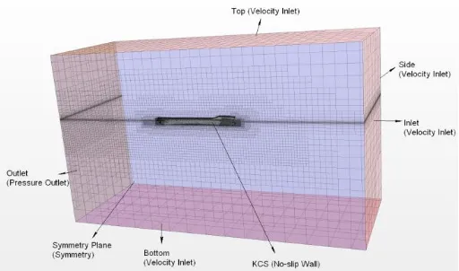
The initial conditions and boundary conditions are defined to represent the KCS ship being towed in deep water. A velocity inlet boundary condition was set at 1.5LPP ahead of vessel and a pressure outlet was selected at 2.5LPP behind. The top and bottom boundaries were both modelled as velocity inlets. A symmetry plane was used to reduce the number of cells and computational demand using a symmetry boundary condition. These boundary conditions were selected by following best practices for similar simulations as recommended by Cd-Adapco [11]. Figure 2 shows an overview of the computational domain with KCS model and selected boundary conditions.

The domain size and location of boundaries are summarized in the table below.

Table 3 Locations of the boundaries in computational domain

Min Max Note

X -1.5 LPP 2.5 LPP AP is set to 0

Y 0 1.5 LPP Centre line is set to 0

Z 1.5 LPP 1.5 LPP AP is set to 0

Figure 2 Overview of the computational domain

Figure 3 Computational mesh around the hull

Three different meshes were created with constant refinement ratio of √2 as recommended by ITTC procedures [12]. Defining refinement regions around the hull and free surface allows the mesh size to be kept as small as possible. This was done through use of volumetric controls in the expected wake areas. Figure 3 demonstrates the refinement areas around ship hull to capture the free surface and Kelvin wake. Total number of cells in the surface mesh of the KCS hull is also shown in Figure 3 above. The total number of cells and the results for three different meshes are shown in the table below. There is no notable difference in between three different meshes and the results are almost identical with the error for the coarse domain of 3% for total resistance coefficient compared to experimental results.

Table 4 Grid size and results for mesh sensitivity

Parameters Coarse Medium Fine

EFD Number of cells 0.6M 1.3M 3.1M

CT*103 4.32 4.3 4.23 4.41

Trim 0.198 0.198 0.195 0.162

Sinkage -0.006 -0.00598 -0.0059 -0.007

Based on these results it was decided to carry out the trim optimisation study with coarse mesh approach due to the high number of simulations required. The computational mesh was regenerated at each trim condition. Refinements around the bow and stern were adapted according to the trimmed ship position.

Figure 4 Wall y+ value on the hull

The boundary layer was modelled using all y+ wall function option in Star CCM+. Prism layers are placed along the hull surface in order to resolve the boundary layer accurately and to achieve the required wall y+ values. As shown in Figure 4 above the dimensionless wall distance y+ was around 45 for each mesh size which is considered as an appropriate size for the standard k-ε model with all y+ boundary treatment.

RESULTS AND DISCUSSION

Experimental Results

Model tests were performed to obtain resistance curves in each trimmed condition. In this study one draft of 0.144m and speeds corresponding to a Froude number between 0.19 and 0.26 was investigated. In total 6 different trim values were investigated ranging from 0.25 to 0.1 degrees.

Figure 5 Resistance curves comparison at 0.25 degree trim

A small trim angle of 0.25 degree by bow gave the optimum resistance for all speeds as shown in Figure 5. Results indicated 1% decrease in total resistance at this trim. This may be explained due to a small reduction in wetted surface area and improved bulb performance.

Figure 6 Resistance curves comparison at 0.6 degree trim

Figure 7 Resistance curves comparison at 1 degree trim

Although 1 degree trim by bow did not affect the resistance at slower speeds, it starts to increase the total resistance at higher speeds. In contrast, 1 degree trim by stern increased the total resistance significantly due to submergence of transom and increased water line length. In total, 1 degree trim by stern and bow increased total resistance by 8% and 6% respectively at the design speed.

Based on model test results, it can be concluded that trim by stern causes an increase in total resistance for all cases while the optimum trim is found when the ship is trimmed 0.25 degree by bow.

Numerical Results

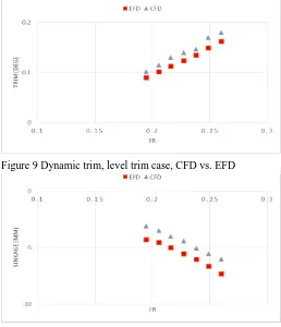
This study also aimed to investigate the effect of incorporating dynamic sinkage and trim into numerical simulation on identifying optimum trim. To this end, first resistance curves were obtained at level trim for various speeds. Dynamic trim and sinkage values were also compared with experimental data (EFD).

Figure 8 shows the comparison between experimental results and CFD calculations for different speeds. It can be seen that CFD results are in good agreement with experimental results with maximum error being 3% for the total resistance. Comparison of numerical and experimental results for sinkage and trim are found to be in reasonable agreement as shown in Figure 9 and 10.

Following validation of numerical method at level trim, the next step is to calculate resistance values at different trim angles. Calculations were carried out for the slow steaming condition at 19 knots and the design speed condition at 24 knots for two different draft values.

.

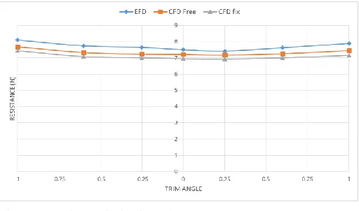
Figure 11 above illustrates the resistance curves at different trim angles. It is clear that trim by stern increases the total resistance of the ship independent of the speed. Percentage differences of total resistance at different trims with respect to total resistance at level trim condition are summarised in Table 5 below.

Figure 8 Total resistance, level trim case, CFD vs. EFD

Figure 10 Dynamic sinkage, level trim case, CFD vs. EFD Figure 9 Dynamic trim, level trim case, CFD vs. EFD

Table 5 Total resistance difference at different trim angles compared to level trim at design draft (10.8 m)

Fn: 0.20 Fn: 0.26 RT difference in % with respect to level trim

Trim (deg) (Positive by bow)

-1 13.235 8.0323

-0.6 5.2622 3.2541

-0.25 1.2713 1.9241

0 0 0

0.25 -1.9216 -1.0876

0.6 -0.6660 1.6519

1 0.3612 5.2898

It can be seen that 0.25 degree by trim can provide 2% reduction in total resistance at 19 knots while reduction potential is 1% at 24 knots. It is possible to say that slow steaming also affects the performance of the ship in the trimmed condition. When the ship is trimmed by stern total resistance increase by 13% at slow steaming condition compared to 8% increase at the design speed. Trimming the vessel by bow performs much better at slow steaming condition with almost no difference in total resistance even at 1 degree trim compared to 5% increase in design speed.

Table 6Total resistance difference at different trim angles compared to level trim at ballast draft (9 m)

Fn: 0.20 Fn: 0.26 RT difference in % with respect to level trim

Trim (deg) (Positive by bow)

-1 8.92 7.12

-0.6 6.5 2.81

-0.25 3.13 0.73

0 0 0

0.25 -2.4 -0.1

0.6 -5.01 -0.12

1 -7.08 -0.18

In ballast draft conditions, trim by bow prove significant reduction in total resistance at slow steaming conditions. At design speed, trim by bow does not provide the same reduction. Trim by stern causes the bulbous bow to emerge above the free surface and thus creates unfavourable bow wave which leads to an increase in ships resistance at both speeds.

Above results prove that effects of trim on ships resistance depend on the vessel speed and the mean draft. Hull form is one of the most important factors with this regard especially in conditions where bulbous bow partially protrude above the water or transom sterns partially immerse.

Table 7 Total resistance values for different trim angles (Positive by bow)

Trim Angle (deg)

-1 -0.6 -0.25 0 0.25 0.6 1

RT EFD (N) 8.09 7.74 7.64 7.50 7.41 7.62 7.89

RT CFD-Free

(N)

7.68 7.33 7.23 7.21 7.16 7.26 7.45

RT

CFD-Fixed (N)

7.44 7.08 7.02 6.94 6.92 7.03 7.16

Table 7 summarises total resistance values for different trim angles. As can be seen, considerable resistance change is observed between fixed ship and free to heave and pitch simulations. The discrepancy of numerical results with respect to experiments is defined by (D-S)/D where D is experimental data and S is simulation data. Free sink and trim model shows 4% discrepancy for the total resistance while fixed model simulation shows 8% difference for the same scenario.

Results from the simulations of fixed and free cases are presented along the experimental results in Figure 11. The free model can accurately predict the 1 % reduction in total resistance when the ship is trimmed 0.25 degree by bow. The fixed model also predicts a reduction; however its magnitude is not predicted as accurately. Comparing the three resistance curves, one can say that both fixed and free trim/sinkage model could predict the trend of resistance with variation of trim angles; however the fixed model fails to measure the absolute values as accurately as the free model did. The fixed model was tested as it is computationally faster and cheaper but results prove that this is an inaccurate approach. Therefore the free sinkage and trim method is a more appropriate technique for trim optimisation.

CONCLUSION

approach and comparisons showed good agreement. The study showed that using simpler technique of fixed trim and sinkage, although reducing computational cost, cannot accurately predict the magnitude of the saving at optimum trim. The model test and CFD method agreed well in prediction of total resistance trend with respect to trim. It was also confirmed that significant reductions in total resistance are achievable by operating the ship at optimum trim.

It was also observed that the resistance can be accurately predicted using a relatively small number of cells with local refinements around the areas of interest. This is especially important for comprehensive trim optimization studies which require high numbers of CFD simulations.

Model tests are valuable in the sense they provide reliable information about the influence of trim on vessels resistance performance. However, creation of a dense knowledge base which includes different speed, trim and draft values within the operational profile of the vessel may take more time and cost than computational methods.

For future work, this study will be further extended to investigate the effect of propeller on the results. More speed and draft conditions will be investigated to create a dense trim optimisation matrix. Full scale simulations will also be carried out in order to investigate scale effects.

ACKNOWLEDGMENTS

The results were obtained using the EPSRC funded ARCHIE-WeSt High Performance Computer, Grant no. EP/K000586/1.

REFERENCES

[1] IMO THE MARINE ENVIRONMENT PROTECTION COMMITTEE (MEPC), "Guidelines for the development of a ship energy efficiency management plan (SEEMP)," Resolution MEPC, 213(63), 2012.

[2] ABS, "Ship Energy Efficiency Measure, Status and Guidance," 2013 .

[3] DNV GL, "EE appraisal tool for IMO," London, 2016. [4] HSH Nordbank, "Expert Market Survey: Eco-Shipping,"

Frankfurt, 2013.

[5] Lemb Larsen N., Simonsen C.D., Klimt Nielsen C., Råe Holm C.., "Understanding the physics of trim," in 9th annual Green Ship Technology Conference, Copenhagen, 2012.

[6] Iavokatos, M. N., Liarokapis, D. E., and Tzabiras, G. D., "Experimental investigation of the trim influence on the resistance characteristics of five ship models," in Development in Marine Transportation and Exploitation of Sea Resources, London, 2014.

[7] J. Sun, H. Tu, Y. Chen, X. De and J. Zhou, "A Study on Trim Optimization for a Container Ship Based on

Effects," Journal of Ship Research, Vol. 60, No. 1 , pp. 30-47, 2016.

[8] ITTC Recommended Procedures and Guidelines, "Example for Uncertainty Analysis of Resistance Tests in Towing Tanks," 2014.

[9] Enger,S., Peric,M., Peric,R., "Simulation of flow around KCS-hull," in Gothenburg 2010-A Workshop on Numerical Ship Hydrodynamics, Gothenburg, 2010

[10] Tezdogan T., Demirel Y.K., Kellett P., Khorasanchi M., Incecik A. and Turan O.:, "Full-scale unsteady RANS CFD simulations of ship behaviour and performance in head seas due to slow steaming," Ocean Engineering, pp. 186-206, 2015.

[11] CD ADAPCO, "User guide STAR-CCM+ Version 11.02.009," 2016.