A theoretical foundation for multi-scale regular vegetation patterns

A theoretical foundation for multi-scale regular vegetation patterns 1

Corina E. Tarnita1,2,*, Juan A. Bonachela3,*, Efrat Sheffer4, Jennifer A. Guyton1, Tyler C. 2

Coverdale1, Ryan A. Long5, Robert M. Pringle1,2 3

4

1

Department of Ecology & Evolutionary Biology, Princeton University, Princeton, NJ 08544, 5

USA 6

2

Mpala Research Center, Box 555, Nanyuki, Kenya 7

3

Marine Population Modeling Group, Department of Mathematics and Statistics, University of 8

Strathclyde, Glasgow, G1 1XH, Scotland, UK 9

4

The R.H. Smith Institute for Plant Sciences and Genetics in Agriculture, The Faculty of 10

Agriculture, Hebrew University of Jerusalem, Rehovot 7610001, Israel 11

5

Department of Fish and Wildlife Services, University of Idaho, Moscow, ID 83844 12

*

Equal contribution. 13

14 15

Self-organized regular vegetation patterns are widespread1 and thought to mediate 16

ecosystem functions such as productivity and robustness2-4, but the mechanisms underlying 17

their origin and maintenance remain disputed. Particularly controversial are landscapes of 18

overdispersed (evenly spaced) elements (Fig. 1), such as North American Mima mounds, 19

Brazilian murundus, South African heuweltjies, and, famously, Namibian fairy circles 20

(FCs)5-13. Two competing hypotheses are currently debated. On the one hand, models of 21

scale-dependent feedbacks (SDF), whereby plants facilitate neighbors while competing with 22

distant individuals, can reproduce various regular patterns identified in satellite 23

imagery1,14,15. Due to its deep theoretical roots and apparent generality, SDF is widely 24

viewed as a unifying and near-universal principle of regular-pattern formation1,16,17 despite 25

scant empirical evidence18. On the other hand, many overdispersed vegetation patterns 26

worldwide have been attributed to subterranean ecosystem engineers such as termites, 27

ants, and rodents3,4,7,19-22. Although potentially consistent with territorial competition 19-28

21,23,24

, this interpretation has been challenged theoretically and empirically11,17,24-26 and 29

(unlike SDF) lacks a unifying dynamical theory, fueling skepticism about its plausibility 30

and generality5,9-11,16-18,24-26. Here we provide a general theoretical foundation for self-31

organization of social-insect colonies, validated using data from four continents, 32

demonstrating that intraspecific competition between territorial animals can generate the 33

large-scale hexagonal regularity of these patterns. However, this mechanism is not 34

mutually exclusive with SDF. Using Namib-Desert FCs as a case study, we present novel 35

field data showing that these landscapes exhibit multi-scale patterning²previously 36

undocumented in this system²that cannot be explained by either mechanism in isolation. 37

These multi-scale patterns and other emergent properties, such as enhanced resistance to 38

and recovery from drought, instead arise from dynamic feedbacks in our theoretical 39

framework that couples both mechanisms. The potentially global extent of animal-induced 40

regularity in vegetation²which can modulate other patterning processes in functionally 41

important ways²underscores the need to integrate multiple mechanisms of ecological self-42

2

Hypotheses about the origin of regularly patterned (i.e., spatially periodic with characteristic 44

cluster size) landscapes are typically presented as strict alternatives, leading to strident and long-45

lasting debates5-12,17,22,28. The Namib FCs provide a fascinating case in point. FCs are bare discs 46

2±35m wide surrounded by rings of tall perennial grasses, found in sandy desert soils along a 47

sliver of southwestern Africa (Figs. 1f, 4a)7,28. Recently, Juergens7 documented strong 48

correlations between FCs and sand-termite (Psammotermes allocerus) activity and proposed a 49

conceptual model in which termites engineer FCs by killing plants, thereby creating bare patches 50

that concentrate moisture7,8. This hypothesis elicited a barrage of counterarguments advocating 51

SDF9-13,18, with debate revolving heavily around the large-scale hexagonal distribution of FCs 52

(each FC has ~6 neighbors on average). It has EHHQ DUJXHG IRU H[DPSOH WKDW VRFLDO LQVHFWV ³DUH 53

not able to create such extremely ordered, and at the same time large-scale homogeneous 54

SDWWHUQV ´ OHDYLQJ 6') DV ³WKH PRVW UHDVRQDEOH ZRUNLQJ K\SRWKHVLV´17. Parallel disputes simmer 55

over the origins of other regular vegetation patterns worldwide, pitting soil fauna versus SDF5. 56

Although often implicitly presented as alternatives, these two mechanisms are not 57

mutually exclusive. Here we reconcile these competing perspectives by theoretically integrating 58

both mechanisms for the first time and testing their predictions against empirical observations. 59

First, we develop a dynamic spatial model to characterize the population dynamics and territorial 60

behavior of a generic soil-nesting social-insect population, showing that intraspecific 61

competition can theoretically generate large-scale hexagonal patterns found in termite mound-62

fields3, heuweltjies22, murundus5, and FCs10. Second, to explore the dynamic interaction and 63

emergent effects of multiple simultaneous self-organization processes, we couple this faunal 64

model to one of SDF-driven vegetation self-organization. We illustrate the power of this merged 65

framework using Namib FCs as a case study: by parameterizing our merged model specifically 66

for that system and testing its predictions against remotely sensed imagery and novel field 67

observations, we show that the interplay of both mechanisms (a) characterizes the vegetation 68

patterns of Namib FC landscapes more completely than either mechanism can in isolation, and 69

(b) predicts the emergence of features in these landscapes that have escaped the notice of prior 70

investigators. This analysis moves beyond dichotomous debates to explore the multi-trophic 71

dynamics and feedbacks that underpin multi-scale regular patterning in complex ecosystems. 72

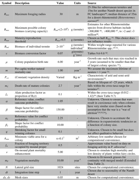
To model social-insect self-organization, we used a spatially explicit model of colony 73

dynamics in a discrete landscape, parameterized from the literature (Extended Data Table 1). 74

Colonies build central nests and forage outwards to acquire resources to fuel colony-population 75

growth and survival. Mature (established) colonies produce alates (reproductive future 76

queens/kings) that disperse randomly throughout our simulated landscapes and attempt to initiate 77

new colonies. Resource availability is constant and uniformly distributed. When the expanding 78

foraging areas of neighboring colonies overlap, conflicts ensue via territorial aggression 79

(Extended Data Fig. 1a), as is common among social insects29. Conflict outcomes depend 80

probabilistically on relative colony size: larger colonies are more likely to eliminate smaller 81

ones, but similar-sized colonies coexist, whereupon a shared boundary emerges (Extended Data 82

Fig. 1b). These conflicts are the primary cause of young-colony mortality (and are intensified by 83

environmental stressors such as drought), while mature colonies have additional probabilistic 84

death rates consistent with typical lifespans reported in the literature. 85

Although this system is intrinsically dynamic due to continual births and deaths of 86

colonies (Supplementary Video 1), the quantities of interest eventually reach stationarity 87

(fluctuating around a well-defined constant average) (Extended Data Fig. 2a,b). We can thus 88

size of mature colonies increased²and mean nest diameter, foraging area, and nearest-neighbor 90

distance decreased²with increasing resource density (Extended Data Fig. 2c-f). This occurred 91

because colonies in resource-rich environments require smaller foraging areas to achieve a given 92

increase in population size. Moreover, colony sizes in low-resource environments were always 93

food-limited (Extended Data Fig. 2f), consistent with prior experimental work20. 94

We quantified predicted nest distributions (Fig. 1a) using standard point-pattern analyses: 95

Voronoi diagrams, pair-FRUUHODWLRQ IXQFWLRQ DQG 5LSOH\¶VL (see Methods). Regardless of 96

resource density, mature nests in our simulations were regularly and hexagonally overdispersed, 97

with ~6 neighbors on average (Fig. 1g-i, Extended Data Fig. 2g). In contrast, immature (typically 98

short-lived) colonies were randomly distributed or clumped, as observed in many ant and termite 99

populations20,21,25,26. These theoretical results correspond well with our analyses of empirical nest 100

distributions for diverse social-insect species from Africa, North and South America, and 101

Australia (Fig. 1, Extended Data Fig. 3,4, Supplementary Text 4.1). Although the degree of 102

hexagonal regularity differs somewhat among sites due to variable topo-edaphic and floristic 103

uniformity, the repeated emergence of such patterns in diverse contexts worldwide²despite the 104

ubiquity of environmental heterogeneity²affirms the generality of the phenomenon27. 105

Our general social-insect model also reproduced the spatial distribution of Namibian 106

FCs10 (Fig. 1f-i, Extended Data Figs. 3,4), showing that the large-scale hexagonal pattern of 107

mature circles and the small-scale heterogeneity of immature circles22,28 can theoretically be 108

explained by termite activity, contrary to recent arguments17. However, this finding does not 109

exclude the possibility that SDF concurrently drives vegetation patterning in this arid system. 110

Therefore, we next developed a theoretical framework incorporating simultaneous social-insect 111

and vegetation self-organization and applied it to the Namib FC system. In the model, termites 112

increase grass mortality on/around nest sites7,8 and forage on dead biomass in the surrounding 113

matrix. To model vegetation (parameterized as a generic tussock grass, like the Stipagrostis spp. 114

bushman-grasses that dominate the Namib), we modified a widely-used partial-differential-115

equation SDF model15 previously applied to Namib FCs9,10 by (a) incorporating stochastic 116

rainfall, based on 10-year records from NamibRand Nature Reserve (Extended Data Fig. 5) and 117

(b) allowing for asymmetric root-biomass growth and water uptake in areas with higher moisture 118

concentrations. We parameterized this model using appropriate values from the literature 119

(Extended Data Tables 1,2). 120

In this coupled model, termites and vegetation dynamically self-organize and interact. 121

Bare FC discs with elevated soil moisture emerge around nests under arid conditions (Fig. 2, 122

Extended Data Fig. 6). If rainfall increases, however, plant regeneration outpaces termite-123

induced mortality, and FCs revegetate (Extended Data Fig. 7), possibly explaining why FCs are 124

absent from Psammotermes nests in mesic regions17 (moisture-mediated plasticity in termite-125

foraging behavior has been suggested as another explanation22). Asymmetric root-biomass 126

growth and water uptake by plants surrounding the moisture-rich bare discs (Fig. 2d,e) promotes 127

HPHUJHQFH RI GHQVH WDOO JUDVV ULQJV OLNH WKH )& ³SHUHQQLDO EHOWV´7 (Fig. 2b,c,f), an important 128

feature not predicted by prior SDF models9,10. FC life cycles emerge in our model, driven by 129

colony establishment, growth, and death (Fig. 3, Supplementary Video 2). FCs emerge quickly 130

following colony establishment, but disappear more slowly after colonies die (Fig. 3k-p) as 131

grasses invade and eventually fill the bare patches (Fig. 3, Extended Data Fig. 6e,f). The weakly 132

bimodal distribution of lifespans ranges broadly from <5 to >165 years (Extended Data Fig. 8), 133

with a peak at <15y and another at ~30±60y, consistent with the existing range of empirical 134

4

criteria proposed to characterize the Namib FC system6,7,12,17,22. 136

Our coupled model also predicts a previously unrecognized feature of the Namib 137

landscape. Prior studies have focused exclusively on the FCs and largely ignored the matrix in 138

between. In our model, SDF induces dynamic self-organization of the matrix vegetation, but at 139

smaller spatial scales more compatible with ecohydrologically realistic grass-water feedback 140

distances (Supplementary Video 3). Following wet seasons, small, regular clumps of matrix 141

vegetation emerge, interspersed with larger, randomly distributed clumps (Fig. 2c). These larger 142

clumps are rare in the SDF-only model without termites, but arise in the coupled model from 143

small-scale soil-moisture variability in the matrix (Fig. 2d; consistent with data22)²itself a ripple 144

effect created by the FCs (Extended Data Fig. 6). To evaluate these theoretical predictions, we 145

photographed NamibRand matrix-vegetation distributions from 10-m height in February 2015 146

and characterized both model-predicted and observed patterns using Fourier-transform analyses 147

(see Methods). We found strong agreement between model outputs and field data (Fig. 4). 148

Thus, by treating SDF and faunal engineering as complementary processes rather than 149

competing alternatives, our model achieves the most comprehensive and realistic description of 150

this system to date. Whereas prior SDF models can reproduce only the formation and qualitative 151

dynamics of hexagonally patterned bare discs9,10,13, our incorporation of termite self-organization 152

and its feedbacks with SDF yields emergent properties absent from prior models but present in 153

the real landscape, including vegetation size structure and the hitherto undocumented small-scale 154

patterning of matrix vegetation. 155

Finally, we asked how the interplay of faunal engineering and SDF influenced ecosystem 156

responses to climatic perturbations. Simulated drought (20% reduction in rainfall sustained over 157

1, 5, or 10 years) reduced system-wide vegetation biomass, but these losses were smaller (i.e., 158

landscapes more drought-resistant) when termites were present. This occurred because the 159

densely vegetated rings and large matrix tussocks generated by the termite-SDF interaction are 160

more drought-resistant and persist after the small matrix patches disappear. Returning rainfall to 161

baseline after drought enabled regeneration of matrix vegetation in both systems; however, 162

recovery occurred faster in the coupled termite-SDF system, because the perennial rings and 163

large matrix clumps act as drought refugia and post-drought sources (Supplementary Video 4). 164

Thus, plant-water-consumer feedbacks sustain the productivity of the Namib by enhancing both 165

its resistance to and recovery from climatic perturbations, as recently hypothesized7. 166

Collectively, our results not only show that interactions among social-insect colonies and 167

vegetation can explain a diverse global suite of regular spatial patterns, but also underscore the 168

potential for co-occurrence and complementarity among distinct patterning mechanisms in 169

generating multi-scale regularity4,30. This highlights the need to focus theoretical and empirical 170

effort on the ways in which multiple mechanisms interact across scales to structure ecosystems27. 171

Advances in remote sensing have buoyed the study of ecological self-organization, but remain 172

insufficient to reveal small-scale patterns. Likewise, evaluating the causes of particular patterns 173

and elucidating multi-mechanism feedbacks will require manipulative field experimentation and 174

8and competitive dynamics of cryptic ecosystem-engineer species; the ways in which plants and 175

SDF respond to bioturbation and climatic variability; and the movement of water through soil in 176

different environmental contexts. Equipped with such knowledge, it may be possible to identify 177

reliable signatures of different mechanisms and specify the scales at which they act and interact. 178

1. Rietkerk, M. & van de Koppel, J. Regular pattern formation in real ecosystems. TREE 23, 181

169±175 (2008). 182

2. Scheffer, M. et al. Early-warning signals for critical transitions. Nature 461, 53±59 183

(2009). 184

3. Pringle, R. M., Doak, D. F., Brody, A. K., Jocqué, R. & Palmer, T. M. Spatial pattern 185

enhances ecosystem functioning in an African savanna. PLoS Biol. 8, e1000377 (2010). 186

4. Bonachela, J. A. et al. Termite mounds can increase the robustness of dryland ecosystems 187

to climatic change. Science 347, 651±655 (2015). 188

5. Cramer, M. D. & Barger, N. N. Are mima-like mounds the consequence of long-term 189

stability of vegetation spatial patterning? Palaeogeogr. Palaeocl. Palaeoecol. 409, 72±83 190

(2014). 191

6. Tschinkel, W. R. The life cycle and life Span of Namibian fairy circles. PLoS ONE 7, 192

e38056 (2012). 193

7. Juergens, N. The biological underpinnings of Namib Desert fairy circles. Science 339, 194

1618±1621 (2013). 195

8. Vlieghe, K., Picker, M., Ross-Gillespie, V. & Erni, B. Herbivory by subterranean termite 196

colonies and the development of fairy circles in SW Namibia. Ecol. Entomol. 40, 42±49 197

(2015). 198

9. Zelnik, Y. R., Meron, E. & Bel, G. Gradual regime shifts in fairy circles. Proc. Natl. Acad. 199

Sci. USA 112, 12327±12331 (2015). 200

10. Getzin, S. et al. Adopting a spatially explicit perspective to study the mysterious fairy 201

circles of Namibia. Ecography 38, 1±11 (2015). 202

11. Getzin, S. et al. Discovery of fairy circles in Australia supports self-organization theory. 203

Proc. Natl. Acad. Sci. USA 113, 3551±3556 (2016). 204

12. Cramer, M. D. %DUJHU 1 1 $UH 1DPLELDQ µIDLU\ FLUFOHV¶ WKH FRQVHTXHQFH RI VHOI-205

organizing spatial vegetation patterning? PLoS ONE 8, e70876 (2013). 206

13. Fernandez-Oto, C., Tlidi, M., Escaff, D. & Clerc, M. G. Strong interaction between plants 207

induces circular barren patches: fairy circles. Phil. Trans. Roy. Soc. A 372, 20140009 208

(2014). 209

14. Meron, E. Modeling dryland landscapes. Math. Model. Nat. Phenom. 6, 163±187 (2011). 210

15. Gilad, E., Hardenberg, von, J., Provenzale, A., Shachak, M. & Meron, E. A mathematical 211

model of plants as ecosystem engineers. J. Theor. Biol. 244, 680±691 (2007). 212

16. Deblauwe, V., Couteron, P., Lejeune, O., Bogaert, J. & Barbier, N. Environmental 213

modulation of self-organized periodic vegetation patterns in Sudan. Ecography 34, 990± 214

1001 (2011). 215

17. Getzin, S. et al. Clarifying misunderstandings regarding vegetation self-organisation and 216

spatial patterns of fairy circles in Namibia: a response to recent termite hypotheses. Ecol. 217

Entomol. 40, 669±675 (2015). 218

18. Tschinkel, W. R. Experiments testing the causes of Namibian fairy circles. PLoS ONE 10, 219

e0140099 (2015). 220

19. Levings, S. C. & Traniello, J. Territoriality, nest dispersion, and community structure in 221

ants. Psyche (1981). 222

20. Korb, J. & Linsenmair, K. E. The causes of spatial patterning of mounds of a fungus-223

cultivating termite: results from nearest-neighbour analysis and ecological studies. 224

Oecologia 127, 324±333 (2001). 225

6

of a mound-building termite species. Insect. Soc. 57, 477±486 (2010). 227

22. Juergens, N. et al. Weaknesses in the plant competition hypothesis for fairy circle 228

formation and evidence supporting the sand termite hypothesis. Ecol. Entomol. 40, 661± 229

668 (2015). 230

23. Laurie, H. Optimal transport in central place foraging, with an application to the 231

overdispersion of heuweltjies. S. Afr. J. Sci. 98, 141±146 (2002). 232

24. Ryti, R. T. & Case, T. J. The role of neighborhood competition in the spacing and 233

diversity of ant communities. Am. Nat. 139, 355±374 (1992). 234

25. Schuurman, G. & Dangerfield, J. M. Dispersion and abundance of Macrotermes 235

michaelseni colonies: a limited role for intraspecific competition. J. Trop. Ecol. 13, 39±49 236

(1997). 237

26. Adams, E. S. & Tschinkel, W. R. Spatial dynamics of colony interactions in young 238

populations of the fire ant Solenopsis invicta. Oecologia 102, 156±163 (1995). 239

27. Pringle, R. M. & Tarnita, C. E. Spatial self-organization of ecosystems: integrating 240

multiple mechanisms of regular-pattern formation. Annu. Rev. Entomol. 62, in press 241

(2017). 242

28. Juergens, N. Exploring common ground for different hypotheses on Namib fairy circles. 243

Ecography 38, 001±003 (2015). 244

29. Thorne, B. L. & Haverty, M. I. A review of intracolony, intraspecific, and interspecific 245

agonism in termites. Sociobiology 19, 115±145 (1991). 246

30. Liu, Q.-X. et al. Pattern formation at multiple spatial scales drives the resilience of mussel 247

bed ecosystems. Nature Commun. 5, 5234 (2014). 248

249

Supplementary Information is linked to the online version of the paper at www.nature.com/nature. 250

251

Acknowledgments: This research is a product of U.S. National Science Foundation grant DEB-252

1355122 to C.E.T. and R.M.P. J.A.B. was supported by the Marine Alliance for Science and 253

Technology for Scotland (MASTS) pooling initiative, funded by the Scottish Funding Council 254

(HR09011) and contributing institutions. WorldView-2 satellite imagery was obtained through a 255

grant from the DigitalGlobe Foundation to R.A.L. We thank: the Government of Namibia and 256

the NamibRand Nature Reserve for permission to conduct research; A. Lamb, D. Doak, G. 257

Barrenechea, P. Davies, S. Levin, R. Martinez-Garcia, I. Rodriguez-Iturbe, A. Sabatino, J. Ware 258

for helpful discussions; I. Arndt for Australian termite-mound images used in analysis and shown 259

in ED Fig. 3; and F. Lanting for connecting us to NamibRand and for use of the image in Fig. 3d. 260

261

Author contributions: C.E.T., J.A.B., and R.M.P. conceived the study and developed the 262

models, with input from E.S. J.A.B performed point-pattern analyses and all simulations. E.S. 263

performed Voronoi and Fourier Transform analyses. J.A.G., T.C.C., and R.A.L. contributed field 264

data and remote-sensing analyses. C.E.T., J.A.B., and R.M.P. drafted the paper, and all authors 265

provided comments. 266

267

Author information: Data are available on Dryad. Reprints and permissions information is 268

available at www.nature.com/reprints. The authors declare no competing financial interests. 269

Correspondence and requests for materials should be addressed to [email protected] and 270

Fig. 1. Social-insect nest distributions, in theory and in nature. a. Model results: dots = 272

centers of mature nest sites; parameterization in Extended Data Table 1. See Supplementary 273

Video 1 for model dynamics. b-e. Remotely sensed images of hexagonal termite and ant nests in 274

(b) Kenya (false-color composite Quickbird satellite image, red circles indicate Odontotermes 275

montanus mound locations); (c) Brazil (Syntermes dirus; GoogleEarth); (d) Arizona, USA 276

(Pogonmyrmex barbatus; GoogleEarth); (e) Mozambique (Macrotermes sp.). Features shown in 277

(b±e) have been ground-truthed as social-insect nests (see Methods and Supplementary Text 4.1). 278

f. Fairy circles (FCs) in Namibia (GoogleEarth). g. Neighbor-number distributions from 279

Voronoi-diagram analysis; bars left-to-right correspond to legend top-to-bottom. h-i. Pair 280

FRUUHODWLRQ DQG 5LSOH\¶VL functions (red curves) for model results (top), Kenya (middle), and 281

FCs (bottom). Shaded areas represent 95% simulation envelopes to discern from complete spatial

282

randomness. Details of images and analyses in Methods and Supplementary Information. 283

284

Fig. 2. Simulation of FC emergence from termite engineering and vegetation feedbacks. a. 285

Termite nest (blue dot) with circular foraging territory. b-c. Characteristic FC vegetation arising 286

around nest site after (b) dry and (c) wet seasons; brown = soil; green = vegetation; darker green 287

indicates greater biomass according to color gradient bar (units = kg/m2). d-f. Predicted soil-288

moisture, root-density, and plant-density profiles along 30-m transects through FCs (0 = nest 289

center). Parameterization in Extended Data Tables 1 and 2. 290

291

Fig. 3. FC life cycle in the coupled termite-vegetation model. a. Nest centers and foraging 292

territories [blue dots = mature colonies; red dots = incipient nests (including the initial diggings 293

of an alate pair)]. b-c. FCs and matrix vegetation following (b) dry and (c) wet seasons; color 294

scheme per Fig. 2b. d. Oblique aerial photo of FCs at NamibRand (image courtesy of Frans 295

Lanting). e-p. Termite-colony dynamics (e-j) and, below each panel, corresponding FC 296

vegetation dynamics (k-p). Red arrow in k-p indicates location of FC shrinkage and 297

disappearance following colony death (red arrow in e). Blue arrow in n-p indicates location of 298

FC appearance and growth following colony establishment (blue arrow in h-j). See 299

Supplementary Video 2 for model dynamics. Parameterization in Extended Data Tables 1 and 2. 300

301

Fig. 4. Predicted and observed regular patterning of FC matrix vegetation. a. Panorama of 302

NamibRand FC landscape showing matrix-vegetation clumps. b. Low-altitude (10-m) 303

photograph of matrix vegetation. Scale bar same as in panel c. c. Model output used for 304

comparison with b. Parameterization in Extended Data Tables 1 and 2. d. Normalized radial 305

spectra of field images (n=27 samples) and model simulations (n=52 samples), as functions of 306

wavenumber. See dynamics of matrix vegetation in Supplementary Video 3. 307

8 313

Methods. 314

Termite dynamics. To characterize the emergent spatial organization of termite nests, we 315

developed a general mechanistic model for termite colony growth, reproduction, foraging 316

behavior, and intraspecific competition (see complete description in the Supplementary 317

Information). For computational convenience, we update these dynamics on a yearly basis. We 318

consider a finite landscape consisting of a regular square lattice. As the initial condition, a single 319

colony founds a nest at a random location within the grid, with a starting population of 2 termites 320

(queen and king) and a minimum viable foraging area Amin. This inaugural colony grows,

321

reproduces, and seeds the rest of the system with new incipient colonies; the system develops 322

with time according to the rules detailed below. Each colony, i, is characterized by its population 323

biomass, Bi(t), and total foraging-territory area, Ai(t).

324

Foraging territory area: Termites forage outward from the nest, which is situated at the 325

center of the initial territory. Thus territories expand in a circular fashion; however, because 326

expansion in certain directions may be blocked by other colonies (see Competition), territory 327

shape does not necessarily remain circular or centered on the nest proper. Ri(t) denotes the

328

largest radial distance within the territory, measured from the center of the nest; this radius is 329

constrained physiologically by Rmax, the maximum distance that a foraging termite can travel.

330

Nest: We assume that the physical nest proper occupies a circular area, Mi(t) (centered at

331

the center of the initial territory), whose radius is a fraction of Ri(t) given by fm.

332

Colony growth: We model colony size and growth in terms of biomass and, consistent 333

with empirical data31, we assume that termite colonies grow logistically. Production of new 334

colony members, P LV GHWHUPLQHG E\ WKH TXHHQ¶V FRQVWDQW UDWH RI HJJ-laying. The carrying 335

capacity, Bmax, represents the maximum possible biomass that a colony can reach, a limit that we

336

assume to be imposed by intrinsic physiological constraints (e.g., how big a nest structure the 337

colony can construct) and thus equivalent for all colonies. Colony members die at a per capita 338

mortality rate m. The effective carrying capacity is therefore Bmax(1 m/µ). To meet basic

339

energetic maintenance costs and achieve growth, colonies require resources. Specifically, the 340

resources needed to maintain colony i at size Bi(t) are given by: éÜ •‡‡† _L

$Ü:P; ?, where c is the

341

termite assimilation capacity (i.e., the conversion factor from resource biomass into termite 342

biomass). This resource requirement is to be compared with the resources available in the 343

foraging territory. Since we model termites that feed exclusively on dead plant material, we 344

assume that resource availability for colony i at time t at any given location x within that 345

FRORQ\¶V WHUULWRU\ LV HTXDO WR WKH DPRXQW RI GHDG SODQW PDWHULDO WKDW KDV DFFXPXODWHG DW WKDW 346

location during the previous year. Assuming that plant mortality occurs at a constant rate, mP,

347

and given that colony i occupies area Ai(t) at time t, the resources available to colony i, Ui(t), are:

348

éÜ:P;L ± ± IÉ2:T&áP";@P"@T& 5›‡ƒ”

ºÔ:ç;

where P(x, t) is the live plant biomass at location x and time t. This will be obtained from the 349

dynamics of the vegetation model below. Because termite dynamics are updated annually, 350

resource requirement and availability are compared at the beginning of each year. If Ui•Uineed,

351

the colony will try to adjust its foraging territory accordingly: if resources are insufficient (Ui <

352

Uineed), the colony will expand its foraging territory trying to obtain the necessary resources;

353

conversely, if resources are in excess (Ui > Uineed), termites will not need to travel as far to harvest

354

the minimum necessary resources, and the foraging territory will shrink. Such shrinkage 355

foraging territory. If territory expansion is hindered for any reason (e.g., lack of available space, 357

or Rmax being reached), then colony biomass will grow only as much as allowed by the resources

358

available up to the point of hindrance. 359

Territorial competition: If territory expansion leads to overlap with the territory of 360

another colony, we assume that a conflict ensues at the border between the two territories in the 361

form of direct interference competition, avoidance, and/or aggressive territorial defense (such 362

antagonism between intraspecific colonies is common among many, perhaps most, species of 363

termites and ants29,32). These conflicts can simply remain as border skirmishes (i.e., offsetting 364

PRUWDOLWLHV QHLWKHU FRORQ\ JDLQV DQ\ QHW JURXQG RU FDQ OHDG WR ³ZDUV´ WKDW PD\ UHVXOW LQ WKH 365

extermination of one colony. We assume that smaller, growing colonies exhibit more 366

aggressively expansionist tendencies than do larger established ones, in keeping with evidence 367

that aggression declines with distance from the nest33 (Fig. S1A). The outcome is probabilistic, 368

with Pr (i and j at war) = Pr (i seeks war) u Pr (j seeks war), where: 369

3U EVHHNV ZDU L

s

sE_A? .k5? .ÌÔ:ç;o ZLWK 5Ü:P;L

$Ü:P;

$PD[

War results either in the death of one colony (highly probable if there is a substantial size 370

discrepancy since we assume ~1:1 mortality in conflict) or in coexistence (if sizes are similar), in 371

ZKLFK FDVH WKH ZRUNHUV¶ IRUDJLQJ UDGLXV LV WUXQFDWHG D ERXQGDU\ LV HVWDEOLVKHG DQG H[SDQVLRQ 372

ceases in that direction. If colonies i and j fight, then i wins with probability: 373

3U:EEHDWVF;L

s

sE_A? :5? ÌÕ:ç; ÌÔ:ç;

If colony i dies in conflict, the winning colony j also suffers losses in the form of reductions in 374

both territory and population biomass: Ajc=Aj Ai, and Bj is reduced proportionally [i.e. Bjc=Bj

375

(Ajc/Aj)]. In the rare event that the winning colony has a smaller territory and biomass than the

376

losing one, then both territory and population biomass are decreased to a fraction q of the 377

original: Ajc=qAj. In either case, the winning area cannot be reduced below the minimum, Amin.

378

Reproduction: We assume that when colonies reach a certain population biomass, Bmat <

379

Bmax, they become reproductively mature (a.k.a. established) and produce alates (winged

380

dispersing future queens and kings) as follows. If, during the current time step, colony i shrinks 381

in biomass due to resource limitation, then it forgoes reproduction even if its newly reduced 382

biomass exceeds Bmat; otherwise, it produces a number of alates proportional to a fraction fA of its

383

biomass. In our simulations we assume that these alates disperse randomly and in pairs over the 384

entire grid. If an alate pair lands within the territory of an established colony or does not have 385

enough space to initiate (i.e., available area at the landing point < Amin), the alates die. Otherwise,

386

they start a new colony. The landing point is assumed to be the center of the new nest. 387

Mortality: There are two sources of mortality for colonies. The first is conflict between 388

neighbors (see above), which we assume to be the primary cause of death in small colonies, but 389

to decline in importance as colonies grow. Indeed, empirical observations from multiple systems 390

suggest that territorial conflict eliminates many incipient colonies but seldom leads to the death 391

of a mature colony, whereas mature colonies show signs of perpetual conflict at outer edges of 392

their foraging territories34-36. The second source of mortality is an intrinsic stochastic death rate, 393

which primarily affects established colonies. We let mC be stochastic mortality for large colonies

394

and set it to replicate a realistic lifetime for mature colonies31,37. 395

Termite engineering: Here, we focus on the scenario in which termites locally deplete 396

plant biomass, as hypothesized for the sand termite Psammotermes allocerus (Rhinotermitidae), 397

10

rate of plant biomass to be elevated by a fixed proportion Q: I_ÉRII LIÉâ IÉ ml Lå IÉRII. For

399

full model details and analysis see SI; for parameterization see Extended Data Table 1. 400

401

Vegetation dynamics. To model vegetation dynamics, we modified a model that has been used 402

repeatedly to describe and reproduce the patterns of self-organization that are typical of 403

vegetation in semi-arid environments15. The model considers the dynamics of vegetation (P), soil 404

water (W), and surface water (O) densities. Assuming a flat terrain, the model can be written as: 405

406

!É:ë&áç;

!ç L)É:T&áP;2:T&áP; @sF É:ë&áç;

Ä AFIÉ2:T&áP;E&ÉÏ

6₂:_T&áP;

(1) 407

!Ð:ë&áç;

!ç LÛ

É:ë&áç;>ÊÐ,

É:ë&áç;>Ê 1:T&áP;F0@sF

ËÐÏàÎÉ:ë&áç;

Ä A9:T&áP;F)Ð:T&áP;9:T&áP;E&ÐÏ

6₉:_T&áP; 408

(2) 409

!È:ë&áç;

!ç L4ÔÜáÙÔßßFÛ

É:ë&áç;>ÊÐ,

É:ë&áç;>Ê 1:T&áP;E&ÈÏ

6:₁6:_T&áP;; ₍₃₎ 410

where’2 represents the nabla operator (second spatial derivative) and the values and meaning of 411

parameters can be found in Extended Data Table 2. The first term in Eq.(3) represents rainfall, 412

the second term represents infiltration of surface water into the soil, and the third term represents 413

water (superficial) diffusion. The first term in Eq.(2) represents the increase in soil water due to 414

infiltration, whereas the second term represents evaporation, the third term represents soil water 415

uptake, and the last term soil water diffusion. Lastly, the first term in Eq.(1) represents plant 416

growth due to water uptake, the second term represents mortality, and the third term vegetation 417

biomass diffusion (via e.g. seed dispersal). In turn, GP and GW, plant growth rate and soil water

418

consumption rate respectively, depend on the extension of the root system. Thus, if the root 419

system is encoded in the kernel: 420

):T&áT&ñáP; L 5

6 Ì_,.‡š’dF

ë&?ë&ñ.

6cÌ,k5>¾É:ë&áç;og

.h (4)

421

the effect of roots on growth and water consumption, respectively, is given by: 422

)É:T&áP;L&ì_Å):T&áT&ñáP;9:T&ñáP;@T&ñ 423

)Ð:T&áP;L ì_Å):T&ñáT&áP;2:T&ñáP;@T&ñ 424

where the integrals consider the totality of the system38. The kernel determines to what extent 425

roots from a body of vegetation biomass (e.g. clump) can use water and influence other parts of 426

the system. Specifically, the Gaussian kernel above sets this distance through its standard 427

deviation, the root-system size, given by 54ksE'2:T&áP;o. 428

Variable rainfall: We used data to replace the constant average rainfall (typically used in models 429

such as the one above) by a more realistic variable rainfall function Rainfall(t) that captures the

430

typical Namib yearly rainfall. To that end, we used data from 2004-2014 from multiple Namib 431

desert locations (provided by Vanessa Hartung) to calculate mean monthly rainfall in a 432

³DYHUDJH´ \HDU DORQJ ZLWK VWDQGDUG HUURUV UHIOHFWLQJ DPRQJ-year variation in monthly totals. The 433

resulting Rainfall(t) depicts the two distinct seasons (wet and dry) characteristic of this region (see

434

Extended Data Fig. 5): 435

4ÔÜáÙÔßß:P;L44sr

qgl@:ß6-₂; A_>sE

êËß:P;? (5)

436

Here, t is the month of the year, and the second term in brackets represents noise (random 437

number uniformly distributed between 0 and VR) that takes into account an additional source of

438

Asymmetric roots: One important feature of the vegetation model above is that the root system 440

represented by the Gaussian kernel, Eq. (4), is symmetric and therefore root density is equivalent 441

in all directions, regardless of heterogeneities in water availability. However, desert-plant roots 442

in sandy substrates both (a) grow preferentially in the direction of localized moisture 443

concentrations (hydrotropism) and (b) exhibit enhanced proliferation, branching, and biomass 444

growth in moist vs. dry soil, breaking the symmetry of root architecture in ways thought to 445

HQDEOH ³SUHFLVH H[SORLWDWLRQ RI ZDWHU SDWFKHV DQG GURXJKW DYRLGDQFH39. We therefore modified 446

the above model to incorporate the possibility of hydrotropism and asymmetric root proliferation 447

(or asymmetric exploitation of soil moisture) in response to localized differences in soil-water 448

availability. Once the soil-moisture difference dissipates, the root system in that direction returns 449

to its original growth pattern. We introduced an additional term in the plant-growth equation, 450

Eq.(1), that modifies plant growth rate by a specific factor. This is calculated by adding to the 451

existing term GP(x,t), an additional contribution from any direction in which soil water surpasses

452

a site-specific threshold, Wth: )èÉ:T&áP;L)É:T&áP;>sEññ(ƒ•›•:T&áP;?, where Zc is a 453

(dimensionless) diminishing factor (in our simulations, Zc = 0.5), necessary to prevent numerical 454

instabilities leading to unrealistic features such as system-wide plant clusters, and Fasym is the

455

improvement function per se, given by: 456

(ƒ•›•:T&áP; LÃ9:T&"áP; 9:T&áP;Äë&ñ

(6) 457

ThH «! V\PERO UHSUHVHQWV VSDWLDO DYHUDJHV DV IROORZV IROORZLQJ (T (4), the standard 458

deviation of the Gaussian root system is given by 54ksE'2:T&áP;o; therefore, a rough estimate 459

of the maximum length of the root system is given by three times that standard deviation. Thus, 460

the spatial averages in Eq. (6) consider locations at a distance T&FT&" Nu₅₄:sE_'2:_T&áP;; and 461

use the immediate neighborhood of these locations to assess the average water availability and 462

how different it is from 9:T&áP;. Because our simulations occur on a square lattice, such spatial 463

average only considers the 4 neighbors of a location T&". However, only nearest neighbors of T&" 464

fulfilling: 465

Ð:ë&ñÙÙáç;

Ð:ë&áç; F9çÛåPr 466

are considered for the average, which ensures that only a sufficiently large contrast between the 467

focal location x and the neighborhood of T&" triggers this differential root growth. In our 468

simulations, we set Wth=4.

469 470

Parameterization and sensitivity analysis. We thoroughly searched the existing literature to 471

identify plausible (and internally consistent) values of individual-, colony-, and population-level 472

parameters such as termite individual biomass, thresholds for maturity and reproduction, as well 473

as the parameters related to the vegetation model (Extended Data Tables 1 and 2). For the latter, 474

we modified prior parameterizations15 to tailor the model to Namib-desert conditions (e.g., the 475

variable rainfall function described above, low surface-water diffusivity). In addition, we 476

conducted sensitivity analyses to test the dependence of the model outputs on each of the 477

different parameters. Finally, because we used a spatial discretization to enhance the speed of our 478

simulations, we conducted additional sensitivity analyses to test the appropriateness of (i) the 479

spatial grain and (ii) topology (square vs. hexagonal lattice) of the underlying grid, showing that 480

these assumptions did not affect the results. 481

482

Insect-nest distributions: field data. We used high-resolution satellite imagery to quantitatively 483

12

mounds in Kenya (Macrotermitinae: Odontotermes montanus; Fig. 1b), Mozambique 485

(Macrotermitinae: Macrotermes spp.; Fig. 1e), Brazil (Termitidae: Syntermes dirus; Fig. 1c), and 486

Australia (Termitidae: Amitermes meridionalis), along with harvester ant nests in the 487

southwestern USA (Formicidae: Pogonomyrmex spp.; Fig. 1d). We further re-analyzed the 488

Namibian FC sites of a prior study10 to ensure concordance and comparability with our other 489

analyses. In all cases, these features were clearly distinguishable in imagery (Fig. 1, Extended 490

Data Fig. 3) and the identities of the insect species that built them have been unambiguously 491

established in published field studies (Supplementary Text 4.1). The regions and locations 492

analyzed are as follows: 493

Kenya²Two topographically, edaphically, and floristically homogeneous rectangular 494

areas (0.975 km2 and 1.201 km2, comprising 205 and 241 mounds, respectively) in clay-rich 495

vertisols DW 0SDOD 5HVHDUFK &HQWUH a ƒ ¶ 1 ƒ ¶ ( ZKHUH RXU SULRU ZRUN KDV H[WHQVLYHO\ 496

ground-truthed mound locations3, from multispectral QuickBird satellite imagery. 497

Mozambique²A subsection of a 0.630-km2 rectangular area of mixed Acacia/palm 498

savanna-woodland in *RURQJRVD 1DWLRQDO 3DUN a ƒ ¶ 6 ƒ ¶ ( FRPSULVLQJ a WRWDO 499

mounds, from multispectral WorldView-2 satellite imagery; this analysis was comprehensively 500

ground-truthed by mapping all mounds on foot. 501

Brazil²Two areas (0.209 and 0.409 km2, comprising ~452 and 751 mounds, 502

UHVSHFWLYHO\ LQ %DKLD 6WDWH a ƒ ¶ 6 ƒ ¶ : IURP *RRJOH (DUWK 503

North America²Two areas of 0.308 and 0.179 km2, comprising ~510 and 224 nests, 504

UHVSHFWLYHO\ LQ $UL]RQD a ƒ ¶ 1 ƒ ¶ : IURP *RRJOH (Drth. 505

Namibia²Three Namib-Desert sites within the Giribes Plain (G) and Marienfluss Valley 506

(MV), within the same rectangular areas analyzed in prior work10, with aerial extents of 0.288 507

(G1), 0.294 (G2), and 0.322 km2 (MV), and comprising 1181, 1288 and 676 FCs, respectively, 508

from Google Earth. 509

Australia²Two oblique aerial photographs (courtesy of photographer Ingo Arndt) of 510

Amitermes mounds in Litchfield National Park, comprising 249 and 295 mounds, respectively. 511

Specific geographic coordinates for these images are unknown, and we were unable to analyze 512

these mounds in satellite images JHQHULF FRRUGLQDWHV IRU /LWFKILHOG DUH a ƒ ¶ 6 ƒ ¶ ( 513

514

Insect-nest distributions: quantitative analysis. We analyzed the spatial distribution of termite 515

PRXQGV DQW QHVWV DQG IDLU\ FLUFOHV KHQFHIRUWK ³SRLQWV´ :H FRPSXWHG 9RURQRL 516

tessellations10,40 for the point patterns, from which we extracted the following information: (1) 517

distributions of nearest-neighbor numbers for each point, i.e., the number of corners of each 518

Voronoi tile, which provides information on the regularity of the pattern (Fig. 1g, Extended Data 519

Fig. 3); (2) distributions of tile areas (mean area and coefficient of variation); and (3) 520

distributions of the distances of all points to their nearest neighbor10. We further calculated 521

SDLUZLVH FRUUHODWLRQ 3&) DQG 5LSOH\¶VL functions41 for each different area (see Supplementary 522

Information and Extended Data Fig. 4 :H XVHG ERWK WKH ³VSDWVWDW´ SDFNDJH41 in R and our own 523

)RUWUDQ FRGH WR FDOFXODWH ERWK IXQFWLRQV :H DOVR XVHG 5¶V ³VSDWVWDW´ IRU WKH FDOFXODWLRQ RI 524

significance envelopes. We used the same approach to analyze the output of the theoretical 525

model (Fig. 1g, Extended Data Figs. 2,3,4). 526

527

Vegetation patterns: field data. We collected low-altitude aerial imagery of Namibian FC and 528

matrix vegetation at the Namib Rand Nature Reserve (NRNR) in southern Namibia (25.04º E, 529

characterized6,7,12. Mean annual precipitation is 70-80 mm6, falling mostly from December-May. 531

The site consists of Kalahari sand plains and dunes typical of the habitat in which Fairy Circles 532

are found6,7,12. The flora is co-dominated by three congeneric bushman-grasses: Stipagrostis 533

obtusa, S. uniplumis, and S. ciliata12. In February 2015, we selected 10 sites spanning ~35km 534

within NRNR. At each site, we haphazardly selected 10 pairs of fairy circles and measured the 535

distance between circles (from one outer ring edge to another) and the size of each FC (average 536

of two perpendicular diameters within the vegetation ring). The mean (± SEM) diameter of FCs 537

in our dataset was 5.94 ± 0.23 m, and the mean distance between circles was 6.9 ± 0.4 m. Low-538

altitude imagery was collected at a subset of three sites: the most northern (24.94º E, 25.95º S), 539

the most southern (25.25º E, 16.02º S), and the most central (25.13º E, 16.01º S). We 540

photographed matrix vegetation at the midpoint between 30 pairs of neighboring FCs (n = 10 541

pairs per site; Fig. 4b) using a digital camera (Canon PowerShot S110), mounted on an 11-m 542

carbon-fiber pole (Ron Thompson Gangster Carp Pole) such that it could be held parallel to the 543

ground at 10-m height. Prior to imaging, we manually removed fallen leaf litter that might have 544

obscured spatial patterns in standing vegetation. Exposure was controlled manually to maintain 545

consistency in changing light conditions. For all images, this camera rig was held at constant 546

height by the same individual (TCC). A reference object was placed in all images and used to 547

scale them to a pixel size of 0.333 cm. 548

549

Vegetation patterns: quantitative analysis. Images were scaled and a large rectangular sub-550

area of similar size (1340 × 1340 pixels for two sites, and 900 × 900 pixels for a site in which 551

fairy circle density was higher) was selected from each image to comprise only grass and soil 552

(i.e., no fairy circles) and no visible disturbance (n=27 images; three of the images were 553

excluded because they did not have a large enough area between circles). Images were processed 554

as in4. For comparison with the model simulations with stochastic seasonal rainfall, we selected 555

snapshots of the simulated vegetation in the wet season in different years (we used snapshots 556

from February, corresponding to when the field images were collected in 2015). From these 557

snapshots, we selected 2 subsections (73 × 73 and 135 × 135 pixels) between neighboring FCs (n 558

= 52, 26 years × 2 subsections year-1). We transformed the patterns of biomass density from the 559

model into binary images (vegetation vs. bare soil; see Fig. 4c) according to a lower threshold

560

found from temporal and spatial analyses of the model data (0.015 Kg/m2). We used the two-561

dimensional (2D) Fourier transform and a subsequent computation of the 2D periodogram (i.e., 562

power spectrum42), to provide a quantitative characterization of the spatial patterns43. We then 563

calculated the radial spectrum r (sum of the periodogram values on concentric ring-shaped 564

regions of the 2D surface), to quantify the portion of image variances that can be accounted for 565

by a simple cosine wave repeating itself r times (wavenumber) along a travel direction of the 566

periodogram. We normalized the radial spectra for: (a) wavenumber, by dividing r by the size of 567

the domain in the analyzed image (ca. 4.45 and 3 m for field images and 3.65 to 6.75 m for 568

simulations); and (b) amplitude of the radial spectrum, by dividing by the maximum of the mean. 569

570

31. Collins, N. M. Populations, age structure and survivorship of colonies of Macrotermes 571

bellicosus (Isoptera: Macrotermitinae). J. Anim. Ecol. 50, 293±311 (1981). 572

32. Holldobler, B. Territoriality in ants. Proc. Amer. Phil. Soc. 123, 211±218 (1979). 573

33. Adams, E. S. Territory size and shape in fire ants: a model based on neighborhood 574

interactions. Ecology 79, 1125±1134 (1998). 575

14

the termite Macrotermes michaelseni in Kajiado, Kenya. J. Zool. 198, 237±247 (1982). 577

35. Palmer, T. M. Wars of attrition: colony size determines competitive outcomes in a guild of 578

African acacia ants. Anim. Behav. 68, 993±1004 (2004). 579

36. Abe, T., Bignell, D. E. & Higashi, M. Termites: Evolution, Sociality, Symbioses, Ecology. 580

(Springer, 2000). 581

37. Keller, L. Queen lifespan and colony characteristics in ants and termites. Insect. Soc. 45, 582

235±246 (1998). 583

38. Gilad, E. & von Hardenberg, J. A fast algorithm for convolution integrals with space and 584

time variant kernels. J. Comput. Phys. 216, 326±336 (2006). 585

39. Guevara, A. & Giordano, C. V. Hydrotropism in lateral but not in pivotal roots of desert 586

plant species under simulated natural conditions. Plant and Soil 389, 257±272 (2014). 587

40. Illian, J., Penttinen, A., Stoyan, H. & Stoyan, D. Statistical Analysis and Modelling of 588

Spatial Point Patterns. (John Wiley & Sons, Ltd, Chichester, UK, 2008). 589

41. Baddeley, A., Rubak, E. & Turner, R. Spatial Point Patterns: Methodology and 590

Applications with R. (Chapman and Hall/CRC, 2015). 591

42. Mugglestone, M. A. & Renshaw, E. Detection of geological lineation on aerial 592

photographs using two-dimensional spectral analysis. Comput. Geosci. 24, 771±784 593

(1998). 594

43. Couteron, P. & Lejeune, O. Periodic spotted patterns in semi‰arid vegetation explained by 595

a propagation‰inhibition model. J. Ecol. 89, 616±628 (2001). 596

44. Tschinkel, W. R. The foraging tunnel system of the Namibian desert termite, 597

Baucaliotermes hainesi. J. Insect Sci. 10, 65 (2010). 598

45. Baker, P. B. & Haverty, M. I. Foraging populations and distances of the desert 599

subterranean termite, Heterotermes aureus (Isoptera: Rhinotermitidae), associated with 600

structures in southern Arizona. J. Econ. Entom. 100, 1381±1390 (2007). 601

46. Jones, S. C. Colony size of the desert subterranean termite Heterotermes aureus (Isoptera: 602

Rhinotermitidae). Southwest. Nat. 35, 285±291 (1990). 603

47. Haagsma, K. A. & Rust, M. K. Colony size estimates, foraging trends, and physiological 604

characteristics of the western subterranean termite (Isoptera: Rhinotermitidae). Environ. 605

Entomol. 24, 1520±1528 (1995). 606

48. Grace, J. K., Abdallay, A. & Farr, K. R. Eastern subterranean termite (Isoptera: 607

Rhinotermitidae) foraging territories and populations in Toronto. Canad. Entomol. 121, 608

551±556 (1989). 609

49. Husseneder, C., Powell, J. E., Grace, J. K., Vargo, E. L. & Matsuura, K. Worker size in 610

the Formosan subterranean termite in relation to colony breeding structure as inferred 611

from molecular markers. Environ. Entomol. 37, 400±408 (2008). 612

50. Wood, T. G. & Sands, W. A. The role of termites in ecosystems. In Production Ecology of 613

Ants and Termites (ed. Brian, M. V.) pp. 245±292 (Cambridge Univ. Press, 1978). 614

51. Matsuura, K. Colony-level stabilization of soldier head width for head-plug defense in the 615

termite Reticulitermes speratus (Isoptera: Rhinotermitidae). Behav. Ecol. Sociobiol. 51, 616

172±179 (2002). 617

52. Darlington, J. P. E. C. Turnover in the populations within mature nests of the termite 618

Macrotermes michaelseni in Kenya. Insect. Soc. 38, 251±262 (1991). 619

53. Hadley, N. F. & Szarek, S. R. Productivity of desert ecosystems. BioScience 31, 747±753 620

(1981). 621

caste in termites: influence of intraspecific competition and accelerated inheritance. Proc. 623

Natl. Acad. Sci. USA 100, 12808±12813 (2003). 624

55. Golodets, C. et al. Climate change scenarios of herbaceous production along an aridity 625

gradient: vulnerability increases with aridity. Oecologia 177, 971±979 (2015). 626

56. Cain, M. L. & Damman, H. Clonal growth and ramet performance in the woodland herb, 627

Asarum canadense. J. Ecol. 85, 883±897 (1997). 628

57. Milton, S. J. & Dean, W. Disturbance, drought and dynamics of desert dune grassland, 629

South Africa. Plant Ecol. 150, 37±51 (2000). 630

58. Evangelides, C., Arampatzis, G. & Tzimopoulos, C. Estimation of Soil Moisture Profile 631

and Diffusivity Using Simple Laboratory Procedures. Soil Sci. 175, 118±127 (2010). 632

59. Danin, A. Plants of Desert Dunes (Springer Science & Business Media, 2012). 633

60. Sheffer, E., Yizhaq, H., Shachak, M. & Meron, E. Mechanisms of vegetation-ring 634

formation in water-limited systems. J. Theor. Biol. 273, 138±146 (2011). 635

636

Data availability statement. The datasets generated and analysed during the current study are 637

available in the Dryad repository. The computer code is available from the corresponding authors 638

upon request. 639

640

Extended Data Figure Legends 641

642

Extended Data Figure 1. Probability functions associated with conflicts in the termite 643

model. a. probability for colony i and colony j WR HQJDJH LQ D ZDU DV D IXQFWLRQ RI HDFK FRORQ\¶V 644

population biomass. b. If colonies i and j engage in a war, probability function for colony j to 645

win the war as a function of the ratio of colony population biomass. 646

647

Extended Data Figure 2. Results of the termite self-organization model with a fixed 648

resource density level, Pcst. a-b. Temporal behavior of mature colonies in the termite model for 649

Pcst = 50 g/m2. a. Average diameter of mature nests (blue shading represents

r

650

distance between nearest neighbors, (where neighbors are nests that share territory borders). Both 651

observables reach a clear stationary state after a transient period of ~200 years. c-f. Emergent 652

behavior for the colonies at the stationary state as a function of the (annually) available level of 653

resources. c. Average mound diameter, which reflects foraging-territory area, decreases as 654

resource availability increases. d. Mean nearest-neighbor distance also decreases with increasing 655

resource density. e. Termite population density (# of individuals/m2) increases with available 656

resources. f. Average colony biomass density (individuals/colony) increases with available 657

resource density, and reaches a saturation value around Bmax(1 m/µ) (see Supplementary

658

Information). g. Frequency distribution of neighbor numbers from Voronoi analysis for the 659

model with different resource densities (inset: mean number of neighbors). Higher resource 660

densities result in a higher number of colonies (numbers in parentheses in the legend) and 661

therefore more powerful results. Results are obtained by averaging over 100 simulations for each 662

resource level; error bars show ± 1 SD. 663

16

Extended Data Figure 3. Average number of neighbors in various field locations. Upper left 665

panel: Average number of neighbors (± 1 SD) from Voronoi analysis of model and field data; 666

number of nests at each location is shown in parentheses. All other panels: Satellite imagery 667

and/or photographs used for data analysis. Mounds are highlighted for ease of observation. If a 668

white rectangle is present then only the points within the rectangle were analyzed; otherwise, the 669

whole image was analyzed. Scale bars = 100m. (Aerial imagery of Amitermes mounds in 670

Australia courtesy of Ingo Arndt. Satellite imagery: Kenya (QuickBird); Mozambique 671

(WorldView-2); all others are from Google Earth. 672

673

Extended Data Figure 4. Spatial point-pattern analyses of various field locations. Left: Pair 674

correlation function as a function of distances between nests. Right: 5LSOH\¶VL function for the 675

same examples. 95% pointwise simulation envelopes (shaded areas) were calculated using the

676

default function from the R package spatstat. These envelopes allow us to reject the null

677

hypothesis (complete spatial randomness) at a confidence level of 95%; thus, if the focal

678

function (red line) falls out of the envelope for a given distance r, the function differs from the

679

expectation for a completely-random point distribution. Both sets of panels show peaks (left 680

panels) or valleys (right panels) of regularity that indicate the presence of overdispersion for each 681

of these examples. Note the different number of nests present in the samples from each location 682

(Extended Data Figure 3), which leads to different levels of noise in the calculation of the two 683

statistics. 684

685

Extended Data Figure 5. Rainfall data from NamibRand. Top: 10-year time-series of 686

monthly rainfall totals 2004-2014, averaged across multiple sites within NamibRand Nature 687

Reserve (data provided by Vanessa Hartung). Bottom: Mean monthly rainfall (i.e., averaged for 688

each month across all years) in NamibRand from 2004-2014 (green line, ± 1SD in red) and 689

proposed rainfall function (blue). The noise term included in Rainfall(t) [Eq.(5) in Methods]

690

ensures that the rainfall function variability is high during the rainy season and low in the dry 691

season, consistent with the data. 692

693

Extended Data Figure 6. Vegetation dynamics with and without termite engineering. a-b. 694

Comparison of the stationary pattern obtained with the vegetation model alone using a. the 695

original symmetric implementation for the root kernel and b. the modified root kernel that is 696

allowed to grow asymmetrically; c-d. Stationary pattern obtained with the naïve setup (i.e. one 697

single, static colony in the center of the system; constant rainfall); c. the resulting pattern using 698

the original, symmetric root kernel; d. the pattern obtained when the asymmetric root system 699

growth is implemented; e-f. Simulation run measuring the recovery time after the death of a 700

colony in the coupled model with variable rainfall and asymmetric roots. e. System a few months 701

before reaching stationarity; a ring of taller and denser vegetation is formed around the gap, and 702

matrix vegetation is reaching its stationary clumpy distribution. f. Several decades after colony 703

death, the gap closes fully, and the remaining large matrix clumps disappear shortly thereafter. 704

Brown = soil; green = vegetation. Color intensity indicates vegetation density. Parameters are as 705

in Extended Data Tables 1 and 2. 706

707

Extended Data Figure 7. The effect of decreasing termite-induced plant mortality or 708

rainfall is high, vegetation growth outpaces termite engineering and, consequently vegetation is 710

found also on nests, disrupting (and for high enough rainfall values completely removing) the 711

bare discs. a. Low mortality enhancement (Q = 1.1); b. Intermediate mortality enhancement (Q = 712

1.25); values in (a-b) are both lower than in Extended Data Table 1 but have same average 713

rainfall as Extended Data Fig.5; c. Intermediate mortality enhancement (Q = 1.25) and average 714

rainfall increased by 10%. Brown = soil; green = vegetation. Color intensity indicates vegetation 715

density. d-f. Corresponding underlying termite territories and nests. Blue dots = established 716

nests; red dots = incipient nests (including the initial diggings of an alate pair, leading to 717

occasionally high local densities as shown in f). Snapshots taken for a peak in vegetation after 718

the system has reached stationarity. Rest of the parameters as in Extended Data Tables 1 and 2. 719

720

Extended Data Figure 8. Distribution of FC lifetimes measured in the coupled model. For n 721

= 9 replicates of the merged model, we kept track for ~300 years (until the end of the simulation) 722

of 100 randomly selected FCs that were born after the stationary state (reached after ~100 years). 723

53 of these FCs disappeared before the end of the simulation, allowing lifespan estimates for that 724

subset. The resulting lifespans range from <5 years to >165 years, within reported estimates for 725

Namib FCs. Note that the distribution is truncated on the right tail due to the limit of available 726

simulation times; however, the overall shape of the distribution should not be strongly affected 727

2

b

e

f

d

c

Distance (m)

Pair correlation function Ripley_·s _L

Model

Kenya 2

Namib G2

0 20 40 60 80 100 120 0 20 40 60 80 100 120 0.2

0.6 1 1.4 0.6 1 0.2 0.6 1 1.4

0 -2 -4 -6 -8 2 0

-10

-20 0 -0.4 -0.8 -1.2 0.4

Number of neighbors

g

100m

100m

40 80 120 160 2 4 6 8 10 12

1.4

40 80 120 160 2 4 6 8 10 12

100m

100m

3 4 5 6 7 8 9 10

0.0 0.1 0.2 0.3 0.4 0.5

i

h

0.2

f

g

h

i

j

k

yr 0

l

yr 7

m

yr 13

n

yr 18

o

yr 21

p

e

5m

c

d

b

a

10m

0.7

0.6

0.5

0.4

0.3

0.2

0.1

1

Supplementary Information for

2

A theoretical foundation for multi-scale regular vegetation patterns

4

Corina E. Tarnita1,2,*, Juan A. Bonachela3,*,, Efrat Sheffer4, Jennifer A. Guyton1, Tyler C. 5

Coverdale1, Ryan A. Long5, Robert M. Pringle1,2 6

7

correspondence to: [email protected], [email protected] 8

9 10

This supplement contains detailed descriptions of the self-organization models for termites 11

(section 1), vegetation (section 2), and termites and vegetation combined (section 3), along with 12

methods and protocols for collection of empirical data (section 4) and data analysis and 13

comparison with model outputs (section 5). Our models apply generally to territorial, central-14

place-foraging social insects; throughout the below, however, we refer interchangeably to 15

“termites” (in lieu of the more generic “social insects”), both for convenience and because most 16

of the empirical systems under investigation (and hence our parameterizations) involve termites. 17

18

1. Termite self-organization model 19

20

To characterize the emergent spatial organization of termite nests, we developed a general 21

mechanistic model for termite colony growth, reproduction, foraging behavior, and intraspecific 22

competition. For computational convenience, we update these dynamics on a yearly basis. The 23

basic elements of the model are: 24

25

Landscape and initial condition. We consider a finite landscape consisting of a regular square 26

lattice—i.e., an N ! N grid mesh with discrete positions (sites) equally spaced by a horizontal

27

distance dx and a vertical distance dy=dx. This discretization, which uses a very fine spatial grain 28

relative to the landscape and to colony sizes (Extended Data Table 1), allows for considerably 29

faster simulations without, in our case, any loss of accuracy (see sensitivity analysis discussion 30

immediately prior to section 1.1 below). As the initial condition, a single colony founds a nest at 31

a random location within the grid, with a starting population of 2 termites (queen and king) and a 32

minimum viable foraging area Amin. This inaugural colony grows, reproduces, and seeds the rest

33

of the system with new incipient colonies; the system develops with time according to the rules 34

detailed below. 35

36

Colony. Each colony, i, is characterized by its population biomass, Bi(t), and total foraging-37

territory area, Ai(t). Because we assume the biomass of each individual to be equal and constant

38

(Bind), keeping track of the population biomass also provides the trajectory of the number of 39

individuals for the colony, i.e. colony size or population size (see full list of parameter values 40

and units in Extended Data Table 1). 41

42

Foraging territory area. Termites forage outward from the nest, which is situated at the center of 43

the initial territory. Thus territories expand in a circular fashion; however, because expansion in 44

certain directions may be blocked by other colonies (see Competition), territory shape does not

45