Assessment of wavelet-based representation techniques for the characterization of stochastic processes modelling pulse-like strong ground motions

      

City, University of London Institutional Repository

Citation

:

Giaralis, A. & Lungu, A. (2012). Assessment of wavelet-based representation techniques for the characterization of stochastic processes modelling pulse-like strong ground motions. Paper presented at the 6th International ASRANet Conference, 02 - 04 July 2012, Croydon, London, UK.

This is the accepted version of the paper.

This version of the publication may differ from the final published

version.

Permanent repository link:

http://openaccess.city.ac.uk/19267/

Link to published version

:

Copyright and reuse:

City Research Online aims to make research

outputs of City, University of London available to a wider audience.

Copyright and Moral Rights remain with the author(s) and/or copyright

holders. URLs from City Research Online may be freely distributed and

linked to.

City Research Online: http://openaccess.city.ac.uk/ [email protected]

ASSESSMENT OF WAVELET-BASED REPRESENTATION TECHNIQUES

FOR THE CHARACTERIZATION OF STOCHASTIC PROCESSES

MODELLING PULSE-LIKE STRONG GROUND MOTIONS

A. Giaralis, City University London, UK A. Lungu, City University London, UK

ABSTRACT

Recently, the Meyer wavelet packets transform (MWPT), the harmonic wavelet transform (HWT), and the S-transform have been used to process recorded earthquake induced strong ground motions (GMs) in various earthquake engineering and engineering seismology applications. In this paper, the potential of these three wavelet-based time-frequency representation (TFR) techniques to identify and to characterize low-frequency pulse-like content in GMs is assessed. This is achieved by processing ensembles of simulated non-stationary time-histories with known energy content upon appropriately fine-tuning the considered TFRs. Next, the ensemble average wavelet transform is used to characterize the energy distribution of the time-histories on the time-frequency plane, within a Monte-Carlo analysis framework. Specifically, the considered time-histories are realizations of sums of uncorrelated uniformly modulated stochastic processes characterized by analytically known evolutionary power spectra (EPSDs). These EPSDs are judicially defined to model the frequency content of pulse-like GMs. Pertinent numerical results considering EPSDs compatible with the elastic design spectrum of the current European (EC8) aseismic code provisions are included, in which pre-specified pulse-type frequency content is introduced by adding low-frequency "patches of energy". The reported numerical data indicate that the HWT provides for smoother estimates of the considered EPSDs than the MWPT. Further, the S-transform is more accurate than both the HWT and the MWPT in identifying the time location and central frequency of the low frequency components contained in the considered artificial pulse-like accelerograms. Overall, this study sheds light into the challenges of detecting low frequency content “corrupted” by higher frequency components in artificial signals modelling pulse-like accelerograms in an effort to inform best practices in the application of TFR techniques to characterize low frequency pulses in recorded GMs.

1. INTRODUCTION

Strong ground motions (GMs) recorded in the proximity of the seismic faults during an earthquake event may exhibit forward directivity or fling effects. These effects are characterized by one or more long-period, high amplitude pulses which may not be readily distinguishable in the acceleration time-history traces of the GMs (e.g. [1, 2]). In many cases, such long period pulses carry a large fraction of the total energy contained in the ground motion. Consequently, consideration of resonance phenomena suggests that flexible structures located in the proximity of seismic faults and/or structures designed to yield during a major earthquake, may be vulnerable to "pulse-like" GMs.

In this respect, the identification and

characterization of low-frequency pulses in field recorded GMs has attracted the interest of the earthquake engineering research community in recent decades. In this context, several researchers employed various wavelet-based signal processing techniques to detect long period pulses in

near-fault GMs [2-5]. These techniques rely on the decomposition of a given time-history on a family of finite energy oscillatory functions (wavelets), which are localized in time and in frequency [6, 7]. In this manner, a representation of the signal energy distribution on the time-frequency (TF) plane is achieved. However, the thus obtained energy distribution depends heavily on the analytical expression of the adopted wavelets and on the discretization of the TF plane both governed by the uncertainty principle (resolution trade-off between time and frequency) [6]. Consequently, addressing the issue of which

wavelet family better captures/characterizes

salient features of recorded GMs, such as the potential presence of long period, high amplitude pulses is an area of open research (e.g. [4]).

in a Monte Carlo-based framework. This study is motivated by the fact that all three considered TFRs have been successfully employed in the open literature to process field recorded GMs for various purposes [5, 10, 11].

Herein, artificial records generated as

realizations of non-stationary processes

characterized by an analytically known

evolutionary power spectrum (EPSD) on the TF plane are considered [12]. In particular, a special class of non-separable stochastic processes defined as the sum of uniformly modulated non-stationary processes [13, 14] is adopted to model pulse-like accelerograms. The considered records are

analyzed using the aforementioned TFR

techniques to obtain their average energy distribution on the TF plane. These distributions are compared with the underlying EPSDs to gauge

the effectiveness of the considered TFR

techniques to capture the frequency content of the artificial records.

It is emphasized that this work does not aim to a rigorous treatment of the problem of wavelet-based spectral estimation of non-stationary processes (see e.g. [15-17]). Rather, it aims to shed light on the limitations of various commonly used TFR techniques to detect low frequency content “corrupted” by higher frequency components in artificial signals modelling pulse-like accelerograms, in an effort to inform best practices in the application of these techniques to characterize low frequency pulses in recorded GMs.

2. THEORETICAL BACKGROUND

2.1 WAVELET-BASED TIME-FREQUENCY REPRESENTATION TECHNIQUES

Consider a family of “wavelet” functions

defined by scaling via the parameter α (α>0) and

by translating in time t via the parameter b a

zero-mean finite-energy waveform ψ(t) according to the

equation

 

,

1

b a

t b

t

a a

  _  _

 . (1)

The factor 1/ a in the above equation ensures

that all scaled copies of the “mother wavelet”

function ψ(t) have the same energy. Further, let

f(t) be a real finite-energy signal. The continuous

wavelet transform (WT) given by the convolution integral [6, 7]

 

,

 

b a,

 

WT f b a_ f t  t dt









(2)

projects the signal f on the wavelet family ψb,a(t) to

yield a representation in two variables: the scale α

and the time translation b. Given the oscillatory

nature of function ψ(t) (see Figure 2 below), it can

be recognized that by reducing the scale parameter

α the corresponding analyzing wavelets are

“compressed” in time and, thus, their frequency content increases. Further, consideration of higher

values of α, yields wavelets characterized by lower

frequency content. In this regard, the scale

parameter α can be interpreted as being inversely

proportional to an effective “central frequency” characterizing the frequency content of the

wavelet ψb,a(t). The associated constant of

proportionality depends on the particular

analytical form of the mother wavelet [7]. Thus,

for a given scale α, the WT in Eq. (2) “scans” the

signal f for frequency components close to a

certain central frequency along the time axis by

varying the time translation parameter b.

In this context, the WT can be viewed as a

representation of the signal f on the

time-frequency plane. The quality of resolution of this representation depends on the specific set of

values of α and b chosen to “discretize” the

time-frequency plane in a practical numerical context. Furthermore, this resolution depends also on the time and frequency localization properties of the wavelet analyzing functions considered in Eq. (2) governed by the uncertainty principle [7]: better localization in time yields wavelets with a wider frequency band and vice versa. In this work, three different wavelet families briefly reviewed in the remainder of this sub-section are considered.

2.1(a) Meyer wavelet packets transform (MWPT)

Consider a “dyadic” discretization scheme of the time-frequency plane based on the set of scale

parameters αj= 2j (j=0,1,2,…) and translation

parameters bk= αjk (k=0,1,2,...) at each scale level j.

Following this discretization scheme, the WT yields a non-redundant decomposition of the

frequency content of the signal f in “octaves”

followed by downsampling (↓2) [6,7]. Specifically, the LP filter produces “approximation coefficients”

(Aji arrays) of the input signal/array at j level,

while the output of the HP filter are “detail

coefficients” (Dji arrays) containing the high

frequency components at each scale. At the next

level j+1 the aforementioned pair of filters is

applied only to the approximation coefficients

associated with the low frequency content of the jth

scale/octave.

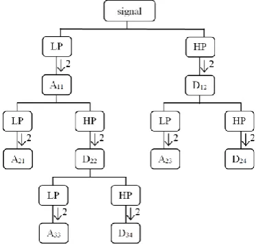
For the purpose of time-frequency signal representation, a more balanced resolution over the whole time-frequency plane than what the DWT offers is desirable. This may be achieved by means of the “wavelet packet transform” (WPT) [7]. In particular, at each scale level WPT

considers the processing of both the Aji and the Dji

[image:4.595.327.558.105.218.2]

arrays as illustrated in Figure 1. In this manner, a “wavelet packet tree” is defined. This is still a non-redundant decomposition with the maximum scale level achieved being dependant on the length of the original signal/array to be processed. Note that the WPT may not be performed to the same scale for the entire frequency bandwidth of the signal. If a more detailed discretization at certain frequency bands is desired, the corresponding “nodes” of the decomposition tree can be further filtered at will as shown in Figure 1. Clearly, this offers a certain degree of flexibility for signal time-frequency representation purposes.

Figure 1. Illustration of a wavelet packet tree decomposition

In this work, Meyer wavelets are used within a wavelet packet decomposition context (MWPT), considered in [5] to process field recorded accelerograms. Meyer wavelets are orthogonal compactly supported in the frequency domain (see Figure 2) resulting in DWT filter banks with some overlapping in the frequency domain between

adjacent scales [18]. The Fourier transform of the Meyer mother wavelet is defined by [7]

 

2

2 ˆ

1 3 2 4

sin 1 ,

2 2 3 3

2

1 3 4 4

cos 1 , ,

2 4 3 3

2

0,

i

i e

e

otherwise







_{ }  _ 

 

_{ }  _ 

 

 

   _  _{ }   _ _

 



 _{ }

  _  _{ }   _ _

 

   

(3)

where the function ν satisfies the conditions

 

0, 0

  

1



1.

1, 0

u

u and u u

u

  _    

 (4)

Figure 2. Mother wavelets (left panels) and their Fourier transform modulus (right panels).

2.1 (b) Harmonic wavelet transform (HWT)

A flexible and straightforward discretization of the time-frequency plane can be achieved by considering the generalized harmonic wavelet transform (HWT) introduced in [8]. Generalized harmonic wavelets are complex waveforms defined in the frequency domain by a band-limited

box-like function (Figure 2). Two parameters (m,n,

with n>m) are used to control the frequency

content of the wavelet instead of a single scale

parameter α. Specifically, the Fourier transform of

a generalized harmonic wavelet at scale (m,n) and

k position in time is defined by [8]

 

,

1

,

, ( )

0, ˆ

i

k m

m

n

kT n

e m n

n m

otherwise



  

 

 



    

   



 (5)

-5 0 5

time

Meyer wavelet

0 5 10

frequency

-5 0 5

time

Harmonic wavelet

0 5 10

frequency

-5 0 5

time

S-transform wavelet

0 5 10

frequency |*()|

(t) |*()|

|*()|

(t)

[image:4.595.326.549.258.484.2] [image:4.595.76.263.487.665.2]

where T is the total length (duration) of the signal f,

Δω= 2π/T and m,n,k are positive integers. It can

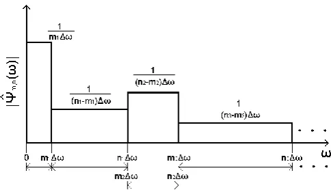
be shown that a collection of harmonic wavelets spanning adjacent non-overlapping bands at different scales along the frequency axis, as shown schematically in Figure 3, forms an orthogonal basis. Focusing on the last figure, it is evident that

a set of mj and nj parameters can be readily chosen

to achieve better frequency resolution (at the expense of a poor time resolution due to the

uncertainty principle) at any band desired. For N

length discrete-time signals, a rather efficient FFT based algorithm exist to compute redundant versions of the underlying HWT where at each

scale N wavelet coefficients equally spaced along

[image:5.595.40.282.320.459.2]

the time axis are computed [8] yielding a rather smooth time-frequency representation of field recorded strong ground motions [10].

Figure 3. Illustration of an orthogonal generalized harmonic wavelet basis.

2.1 (c) S-transform

Introduced in [9], the S-transform can be viewed as a wavelet-based technique for signal time-frequency representation [19] which has been used to process recorded seismic data [20]. The S-transform is defined in terms of the WT by the equation

 

2

 

, ,

b i

a

ST b a e  WT f b a_ , (6) where the following Morlet analyzing wavelet is incorporated in the WT [19]

 

2

2 2 ,

1

2

t b t b i

a a

a b t e e

a









     _ _  _ _

 . (7)

Comparing the last equation with Eq. (1) it can be seen that the S-transform uses a different type of normalization which preserves the amplitude of

the wavelet upon “scaling” (i.e. change of the frequency content), rather than the energy.

2.2 A CLASS OF NON-STATIONARY

RANDOM PROCESSES FOR STRONG

GROUND MOTION REPRESENTATION

For the purposes of this work, the

aforementioned TFR techniques are applied to process realizations (acceleration time-histories) belonging to random processes with a predefined evolutionary (time-varying) frequency content. Specifically, the class of separable

non-stationary random processes x(t) defined as the

sum of R separable (uniformly modulated)

processes xr(t); r= 1,2,…,R, is considered, that is,

 

 

1

R r r x t x t







, (8)

in which

 

   

r r r

x t A t g t . (9)

In the last equation gr(t) is a stationary process

multiplied by a deterministic “envelope” function

Ar(t). For sufficiently slowly varying in time

functions Ar, it can be shown that the energy

distribution of the process x on the time-frequency

plane can be represented by the concept of the evolutionary power spectrum (EPSD) given by the expression [12,14]

 

 

2

1

, _r( )

R r r

S t  A t G 







. (10)

In the above equation Gr(ω) is the power spectrum

of the stationary process gr(t). In this regard, it can

be seen that the frequency content of the process x

is controlled by the R power spectra Gr

contributing to the EPSD of Eq. (10). Further, the intensity and the time variation of each “frequency

contribution” Gr is defined by the corresponding

Ar function.

Stochastic processes of the form of Eq. (8) with various analytically defined expressions for the

envelope function Ar and the power spectrum Gr

have been used in the literature to model the earthquake induced strong ground motion in terms of acceleration for various earthquake engineering applications. For instance, Spanos and Vargas Loli [13] have considered the stochastic model of Eq. (8) for the generation of artificial spectrum

compatible accelerograms in a stochastic

used the aforementioned model for the characterization and representation of certain field recorded accelerograms associated with specific historic seismic events.

In the ensuing numerical applications the bell-shaped envelope function given by [21]

 

2

r

b t

r r

A t C te , (11)

is adopted to account for the commonly observed time-varying pattern in the intensity of recorded earthquake accelerograms (see also [22]). The

values of the constant parameters Cr and br

determine the “height” and the “width” of the adopted bell-shaped function [23]. Consequently, these parameters control the amplitude and the time-domain characteristics (i.e. location of peak

amplitude in time and effective duration) of the rth

spectral contribution in the EPSD of Eq. (10). Further, the Clough-Penzien (CP) spectral form is considered to define the two-sided power

spectrum of the stationary process gr with cut-off

frequency ωc,r given as [24]

 

4

, 2

2 2

2 ,

, ,

2 2

, ,

, 2

2 2

2 ,

, ,

1 4

1 4

,

1 4

f r r

f r

f r f r

g r g r

c r

g r

g r g r

G

  

 _ 

 

 



 

 _ 

 

 

 

 

 



 _{ }  _{ }

 _{ }  _{  }

   

 _{ }  _{ }

 

 

 _ _

 

 

 _{ }  _{ }

 _{ }  _{  }

   

 _{ }  _{ }

 

(12)

The above spectrum is a high-pass filtered version of the Kanai-Tajimi filter [25]: arguably the phenomenological model most extensively used in the literature to represent the frequency content of the strong ground motion due to earthquakes. In

Eq. (12) the parameters ωg,r and ζg,rare related to

the site conditions and represent the “stiffness”

and “damping” of the surface soil layers, while ωf,r

and ζf,r define the frequency response function

properties of the incorporated filter (see also [22] and references therein).

In this junction, it is important to note for the purposes of this work that the stochastic representation of the ground motion expressed by

Eq. (8) allows for the use of power spectrum compatible simulation techniques for stationary processes to generate samples of the non-stationary non-separable process characterized by the EPSD of Eq. (10). An efficient technique for this task is briefly discussed in the following section.

2.3 AN ARMA FILTERING METHOD FOR

GENERATING NON-STATIONARY

NON-SEPARABLE STRONG GROUND MOTIONS

Realizations of the non-stationary

non-separable acceleration strong ground motion

process x of Eq. (8) can be numerically generated

by first considering stationary discrete-time

signals sampled at an interval _s / max

 

_{c r,}

r T  

from the continuous-time stochastic processes gr(t)

appearing in Eq. (9). That is,

 

 

, 0,1,...,

r r s

g s g sT s N. (13)

In practice, the total duration T=NTs should be

defined such that max



_r

 



r A T attains a negligible

non-zero value. Next, these stationary signals from

each process gr are multiplied individually by the

corresponding discrete/sampled version of the

envelope function Ar of Eq. (11) to produce

discrete-time signals xr[s];s=0,1,…,N with

non-stationary intensity as Eq. (9) suggests. Finally,

one such signal from each of the R processes is

chosen; the R chosen signals are summed up to

produce one realization x[s] of the process x

according to Eq. (8). Irrespectively of the random field simulation algorithm used to produce numerically the stationary signals compatible with

the Gr spectra it is important to ensure that these

signals are statistically independent [14].

In this study, stationary discrete-time signals

 

r

g s are synthesized by filtering arrays of

discrete-time Gaussian white noise w[s] with a

two-sided unit-intensity power spectrum

band-limited to ωc,r through an

auto-regressive-moving-average (ARMA) filter of order (P,Q). In a

practical numerical implementation setting these

arrays comprise pseudo-random numbers

belonging to a Gaussian distribution with zero

mean and variance equal to 2c r_, . In this

filtering operation is governed by the difference equation

 









1 0

Q P

r p r q

p q

g s d g s p c w s q

 

 



 



 (14)

in which cq (q=0,1,…,Q) and dp (p= 1,…,P) are

the ARMA filter coefficients. Herein, the auto/cross-correlation matching (ACM) method is adopted to determine these coefficients so that the

power spectrum of the process g s_r

 

matches the

CP spectrum Gr of the process gr[s]. In this

manner, the process g s_r

 

can reliably model the

process gr[s]. The mathematical details of the

ACM method can be found in [26] .

2.4 WAVELET-BASED CHARACTERIZATION OF STOCHASTIC PROCESSES

Let the time-frequency plane be discretized by a

set of dilation and translation parameters (αi and bi,

i=0,1,2,…, respectively) within a wavelet-based

analysis incorporating an orthogonal family of wavelets. Consider the value of an EPSD characterizing a non-stationary stochastic process

at a “central frequency” corresponding to the αj

scale and “time instant” corresponding to the bj

location in time. It can be shown theoretically that for slowly varying EPSDs the mean square modulus of the wavelet transform of the process is proportional to the local value of the EPSD, that is, [16,17,27,28]











2



, , ,

j j j j

S b a E WT x b a_ (15)

where E{∙} is the operator of the mathematical

expectation (i.e. the ensemble average). The above equation is related to a Parseval’s theorem of energy preservation in applying the wavelet transform, which will always hold for orthogonal wavelets. The constant of proportionality depends on the analyzing wavelet used. For example, for

harmonic wavelets at scale (mj, nj) it can be shown

that this constant is equal to (Δω(nj-mj))-1 with αj=

(mj+nj)/2 [29]. The quality of the estimation

depends on the “smoothness” of the considered EPSD and is associated with the concept of locally stationary processes (e.g. [15,17]).

Equation (15) justifies the idea of evaluating numerically the ensemble average of the square modulus of wavelet coefficients by applying the wavelet transform to a large number of

realizations compatible with a specific EPSD in a Monte Carlo based context. In case the aforementioned assumptions are satisfied this average value should compare well with the considered EPSD. Therefore, one can use this numerical experiment to gauge the effectiveness of various wavelet-based analysis techniques to capture the energy distribution on the time-frequency plane of processes with specific evolutionary frequency content. Several such numerical studies have been reported in the literature [16,17,27,28]. The ensuing sections report novel results probing into the detection of low-frequency content in processes modelling pulse-like strong ground motions acceleration traces using the stochastic model discussed in section 2.2.

3. NUMERICAL APPLICATIONS

3.1 SIMULATION OF PULSE-LIKE STRONG GROUND MOTION PROCESSES

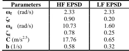
[image:7.595.319.532.639.724.2]

Two uniformly modulated CP processes defined by Eqs. (9), (11), and (12) are considered to represent the “high-frequency” (HF) and the “low-frequency” (LF) content in generating artificial acceleration traces of pulse-like strong ground motions. The parameters for the definition of the underlying EPSDs of these two processes are reported in Table 1. The considered HF EPSD is compatible with the elastic spectrum of the European aseismic code provisions (EC8) [30] for 0.36g peak ground acceleration and soil type B (as classified in EC8) derived in Giaralis and Spanos [31]. Further, the parameters of the LF EPSD are judicially chosen to represent the time and frequency attributes of typical pulses extracted from field recorded accelerograms associated with historic seismic events as reported in the literature ([1,32]).

Table 1. EPSD definition of CP spectral forms

Parameters HF EPSD LF EPSD

ωf (rad/s) 2.33 2.33

ζf 0.90 0.20

ωg (rad/s) 10.73 1.60

ζg 0.78 0.25

C (m/s2.5) 17.76 0.65

b (1/s) 0.58 0.32

of the TFR methods discussed in section 2.1 to characterize the frequency content of pulse-like strong ground motions. The first process is the aforementioned HF EC8 compatible separable

process (R=1 in Eq.(8)) [31]. The second process

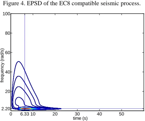
[image:8.595.45.289.327.712.2]

considered is non-separable (R=2 in Eq.(8)) defined as a weighted sum of the HF and the LF EPSDs of Table 1. The “combination rule” applied is 0.30HF+LF which achieves an average energy ratio of the HF over the LF frequency content equal to 0.20. In this manner, a separable non-stationary process with a prominent low-frequency “patch” of energy is defined to model the near-fault pulse-like strong ground motion. Contour plots of the EPSDs of the two considered processes are shown in Figure 4 Figure 5. In the last figures the location of the peak value of these EPSD in time and in frequency is also identified.

Figure 4. EPSD of the EC8 compatible seismic process.

Figure 5. EPSD of the pulse-like seismic process.

Two ensembles of 200 realizations each compatible with the processes of Figure 4 and Figure 5 are generated using the simulation

approach described in section 2.3. A cut-off

frequency ωc= 300rad/s is adopted for the CP

spectra considered and the duration of each realization is set to 60s with a sampling step equal

to π/ωc to avoid aliasing.

3.2 EPSD ESTIMATION VIA THE MWPT AND THE HWT

Both ensembles of realizations/signals

belonging to the EC8 compatible process and to the pulse- like process defined in the previous sub-section are processed using the MWPT and the HWT. Prior to processing, the signals are zero-padded up to the next power of 2 to expedite the numerical implementation and to reduce end-effects [33]. By relying on Eq. (15) and assuming that the considered number of realizations is sufficiently large, the ensemble average of the squared modulus of MWPT and HWT of these signals should compare reasonably well with the corresponding (target) EPSDs of Figure 4 and Figure 5. By “inversion” of the above argument, the herein considered numerical experiment is used to assess the potential of the MWPT and HWT to capture the frequency content of artificial signals with a known frequency content modelling far-field (EC8 compatible process) and near-field (pulse-like compatible process) strong ground motion.

Figures 6 and 7 show contour plots of the MWPT and the HWT estimates of the EC8 compatible EPSD, respectively, obtained as detailed above. In applying the MWPT to the EC8 compatible signals, a wavelet packet tree with a

depth of j= 7 has been considered. In applying the

HWT to the same signals, an orthogonal generalized harmonic wavelet basis with constant

frequency bandwidth of (n-m)Δω=2rad/s spanning

the interval [0, ωc] on the frequency axis was used.

The aforementioned algorithmic parameters have

been selected upon extensive numerical

experimentation considering the quality of approximation in Eq. (15) in terms of energy leakage, EPSD peak location on the time-frequency plane, “ridge” (locus of maxima) of the transform and other pertinent criteria. By comparing the estimated EPSDs of Figures 6 and 7 with the “target” EPSD of Figure 4 it can be argued that a reasonable estimation has been obtained for the selected parameters. A more widespread energy leakage towards higher frequencies is observed in the case of the MWPT

time (s)

fr

eq

ue

ncy

(r

ad

/s)

0 3.45 10 20 30 40 50 60

0 9 20 40 60 80 100

time (s)

fr

eq

ue

ncy

(r

ad

/s)

0 6.33 10 20 30 40 50 2.20

[image:8.595.47.287.327.503.2] [image:8.595.51.286.512.708.2]

compared to the HWT. However, a more eminent shift of the predominant frequencies towards higher values is observed in the HWT case. Overall, the redundant HWT does offer a smoother estimator compared to the

non-redundant MWPT. These are qualitative

observations indicating the challenges in applying any wavelet-based method for signal energy characterization on the time-frequency plane.

[image:9.595.39.281.212.522.2]

Figure 6. EC8 compatible EPSD estimation via MWPT.

Figure 7. EC8 compatible EPSD estimation via HWT.

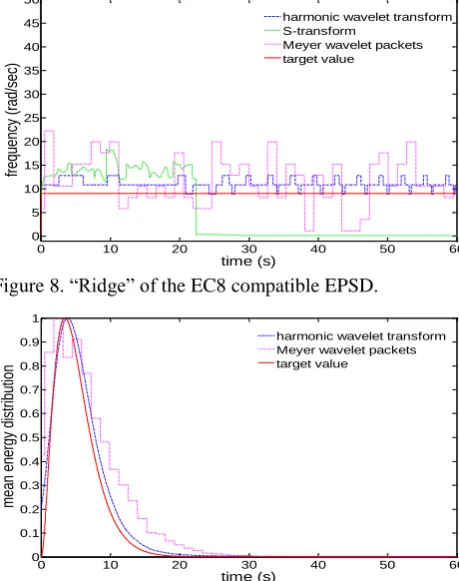
Further, the ridge of the EC8 compatible EPSD estimated via the MWPT and HWT is shown in Figure 8 and compared with the “target value” of 9 rad/s (see also Figure 4). The ridge obtained by the MWPT attains a large variance, although its temporal mean value is satisfactory close to the target one. The ridge obtained by the HWT is shifted on average towards a higher frequency than the target, but it has a much smaller variance around the mean value. Figure 9 plots the time-varying ensemble average energy normalized by its peak value obtained by the MWPT and the HWT together with the “target” curve obtained

[image:9.595.309.539.220.511.2]

from the EC8 compatible EPSD. Clearly, the HWT approximates well the target curve and lies much closer than the estimate obtained by the MWPT. In view of the herein reported numerical data obtained upon calibration of the parameters involved in performing the MWPT and the HWT, it can be argued that the HWT is more accurate in capturing the non-stationary intensity and the constant frequency content of the considered uniformly modulated EC8 compatible process.

Figure 8. “Ridge” of the EC8 compatible EPSD.

Figure 9. Mean energy estimation of the EC8 compatible process.

Figures 10 and 11 show contour plots of the ensemble average of the square modulus of the MWPT and the HWT for the case of the pulse-like process possessing a dominant low-frequency patch of energy centered at 2.20rad/s (Figure 5). In this case, both the MWPT and the HWT have been tuned to achieve higher resolution in the frequency range where the low frequency pulses “live”. Specifically, in applying the MWPT to the artificial pulse-like accelerograms considered, a

wavelet packet tree up to the level j=9 has been

used for the “terminal nodes” corresponding to the frequency band [0,5] (rad/s), while the highest level considered outside this interval has been set

to j=7. Further, in applying the HWT, adjacent

non-overlapping scales of 0.5rad/s and of 2rad/s

time (s)

fr

eq

ue

ncy

(r

ad

/s)

02.52 10 20 30 40 50 60

10.55 20 40 60 80 100

time (s)

fr

eq

ue

ncy

(r

ad

/s)

0 4.30 10 20 30 40 50 60

12.80 20 40 60 80 100

0 10 20 30 40 50 60

0 5 10 15 20 25 30 35 40 45 50

time (s)

fr

eq

ue

ncy

(r

ad

/se

c)

harmonic wavelet transform S-transform

Meyer wavelet packets target value

0 10 20 30 40 50 60

0 0.1 0.2 0.3 0.4 0.5 0.6 0.7 0.8 0.9 1

time (s)

m

ea

n

en

er

gy

distr

ib

ut

io

n

[image:9.595.41.279.391.579.2]

have been considered within and outside the frequency band [0,5] (rad/s), respectively.

[image:10.595.318.550.74.209.2]

It can be readily seen in Figures 10 and 11 that the position of the dominant low-frequency content on the frequency axis is captured very well by both the MWPT and the HWT. However, there is rather poor time localization due to the uncertainty principle in conjunction with the fact that wavelet analysis aiming for higher frequency resolution in low frequencies, as one would intuitively use to detect low frequency pulses in recorded accelerograms, has been employed. Indeed, the value of the dominant (low) frequency content is accurately estimated, as it is confirmed by the ridge of the modulus squared of the MWPT and HWT shown in Figure 12, while its position in time is not identified. In this respect, the herein considered wavelet-based signal processing tools may not be appropriate to locate accurately low-frequency pulses in acceleration traces on the frequency and the time axis simultaneously.

[image:10.595.49.287.362.542.2]

Figure 10. Pulse-like EPSD estimation via MWPT.

[image:10.595.46.273.564.733.2]

Figure 11. Pulse-like EPSD estimation via HWT.

Figure 12. “Ridge” of the pulse-like EPSD.

3.3 ASSESMENT OF THE S-TRANSFORM

FOR LOW FREQUENCY CONTENT

IDENTIFICATION

The S-transform is not energy preserving and, thus, it cannot be used for EPSD estimation as has been the case for the MWPT and the HWT. However, it is herein considered to characterize the energy content of the pulse-like process. To this end, the ensemble of the signals belonging to the latter process is processed via the S-transform. The contour plot of the ensemble average of the modulus of the S-transform of these signals is shown in Figure 13. It can be seen that the S-transform performs better in localizing the low frequency patch of energy in the pulse-like process on the time-frequency plane compared to the MWPT and the HWT. Furthermore, the high frequency content is also well identified. These observations are further confirmed by the ridge of the S-transform included in Figure 12. In this respect, it can be argued that the S-transform may be a potent signal processing tool for identifying low frequency pulse-like content in strong ground motions recorded in the near-fault field.

Figure 13. S-Transform of the pulse-like process. time (s)

fr

eq

ue

ncy

(r

ad

/s)

0 11.24 20 30 40 50 60

2.05 20 40 60 80 100

time (s)

fr

eq

ue

ncy

(r

ad

/s)

0 8 10 20 30 40 50 60

2.28 5 20 40 60 80 100

0 10 20 30 40 50 60

0 1 2 3 4 5 6 7 8 9 10

time (s)

fr

eq

ue

ncy

(r

ad

/sec)

harmonic wavelets transform S-transform

Meyer wavelet packets target spectrum

time (s)

fr

eq

ue

ncy

(r

ad

/sec)

0 7.48 20 30 40 50 60

[image:10.595.317.553.569.745.2]

5. CONCLUDING REMARKS

The potential of three wavelet-based signal processing techniques has been assessed for seismic signal time frequency representation by considering realizations of two non-stationary random processes characterized by analytically known evolutionary power spectra (EPSDs). Specifically, the Meyer wavelet packets transform (MWPT), the generalized harmonic wavelet transform (HWT) and the S-transform have been considered, motivated by the fact that they have been used in the published literature to process field recorded strong ground motions. Special attention has been focused in gauging the

performance of these techniques to

detect/characterize a low-frequency

high-amplitude “patch of energy” in high-frequency “noise” which is observed in certain “pulse-like” near-fault recorded strong ground motions. To this aim, a non-separable non-stationary stochastic process model defined as the superposition of uncorrelated uniformly modulated stochastic processes is used to model the frequency content of pulse-like strong ground motions.

The herein reported numerical data

demonstrates that the redundant HWT performs better than MWPT in obtaining smooth estimates of the considered EPSDs as the ensemble average of the squared modulus of transformed EPSD compatible signals. Furthermore, the S-transform is more accurate than the HWT and the MWPT in identifying the time location and central frequency of the low frequency components contained in the considered artificial pulse-like accelerograms. In this respect, the S-transform might be a promising tool for pulse characterization and extraction in near-fault field recorded accelerograms, if used in tandem with an adaptive signal processing

technique such as the empirical mode

decomposition [34,35].

As a final remark, it is noted that the herein considered model for simulation of pulse-like artificial accelerograms may be a viable alternative to other stochastic models proposed in the literature [1,32] as it furnishes certain

advantages. These include simplicity in

representing the low frequency component and versatility in the representation of the high frequency component which can be chosen to be compatible with specific response/design spectra [31]: a desirable consideration for the earthquake

resistant design of structures located close to active seismic faults.

REFERENCES

1. MAVROEIDIS, G., PAPAGEORGIOU, A.S., 2003, ‘A mathematical representation of near-fault ground motions’,

Bulletin of Seismological Society of America, Vol. 93(3), pp. 1099-1131.

2. BAKER, J.W., 2007, ‘Quantitative classification of near-fault ground motions using wavelet analysis’, Bulletin of the Seismological Society of America, Vol. 97(5), pp. 1486-1501. 3. TODOROVSKA, M.I., MEIDANI, H., TRIFUNAC, M.D., 2009, ‘Wavelet approximation of earthquake strong ground motion-goodness of fir for a database in terms of predicting nonlinear structural response’, Soil Dynamics and Earthquake Engineering, Vol. 29, pp. 742-751.

4. VASSILIOU, M.F., MAKRIS, N., 2011, ‘Estimating time scales and length scales in pulse-like earthquake acceleration records with wavelet analysis’, Bulletin of the Seismological Society of America, Vol. 101( 2), pp. 596–618.

5. YAMAMOTO, Y., BAKER, J.W., 2011, ‘Stochastic model for earthquake ground motions using wavelet packets’,

11th International Conference on Applications of Statistics and Probability in Civil Engineering, Zurich, Switzerland. 6. MALLAT, S., 2009, ‘A wavelet tour of signal processing’,

Academic Press, Burlington, MA.

7. DAUBECHIES, I., 1992, ‘Ten lectures on wavelets’,

Society for Industrial and Applied Mathematics,

Philadelphia, PA.

8. NEWLAND, D.E., 1994, ‘Harmonic and musical wavelets’, Proceedings of the Royal Society of London, Series A,Vol. 444, pp. 605-620.

9. STOCKWELL, R.G., MANSINHA, L., LOWE, R.P., 1996, ‘Localization of the Complex Spectrum: The S-Transform’, IEEE Transactions on Signal Processing, Vol. 44(4), pp. 998-1001.

10. SPANOS, P.D., GIARALIS, A., POLITIS, N.P., ROESSETT, J.M., 2007, ‘Numerical treatment of seismic accelerograms and of inelastic seismic structural responses using harmonic wavelets’, Computer-Aided Civil and Infrastructure Engineering, Vol 22, pp. 254- 264.

11. PAROLAI, S., 2009, ‘Denoising of seismograms using the S-transform’, Bulletin of the Seismological Society of America, Vol. 99(1), pp. 226–234.

12. PRIESTLEY, M.B., 1965, ‘Evolutionary spectra and non-stationary processes’, Journal of the Royal Statistical Society, Series B, Vol.27, pp. 204–237.

13. SPANOS, P.D., VARGAS LOLI, L.M., 1985, ‘A statistical approach to generation of design spectrum compatible earthquake time histories’, Soil Dynamics and Earthquake Engineering, Vol.4, pp. 2-8.

14. CONTE, J.P., PENG B.F., 1997, ‘Fully nonstationary analytical earthquake ground-motion model’, Journal of

Engineering Mechanics, ASCE, Vol.123, pp. 15-24.

17. SPANOS, P.D., KOUGIOUMTZOGLOU, I.A., 2012, ‘Harmonic wavelets based statistical linearization for response evolutionary power spectrum determination’,

Probabilistic Engineering Mechanics, Vol. 27(1), pp.57-68. 18. TEOLIS, A., 1998, ‘Computational Signal Processing with Wavelets’, Birkhauser, Boston, MA.

19. VENTOSA, S., SIMON, c., SCHIMMEL, M., DANOBEITIA, J.J., MANUEL, A., 2008, ‘The S-transform from a wavelet point of view’, IEEE Transactions on Signal Processing, Vol. 56(7I), pp. 2771-2780.

20. PAROLAI, S., 2009, ‘Denoising of seismograms using the S-transform’, Bulletin of the Seismological Society of America, Vol. 99(1), pp. 226–234.

21. BOGDANOFF, J.L., GOLDBERG, J.E., BERNARD, M.C., 1961, ‘Response of a simple structure to a random earthquake-type disturbance’, Bulletin of the Seismological Society of America, Vol. 51, pp. 293–310.

22. GIARALIS, A., SPANOS, P.D., 2009, ‘Wavelets based response spectrum compatible synthesis of accelerograms- Eurocode application (EC8)’, Soil Dynamics and

Earthquake Engineering, Vol.29, pp. 219–235.

23. SPANOS, P.D., GIARALIS, A., JIE, L., 2009, ‘Synthesis of accelerograms compatible with the Chinese GB 50011-2001 design spectrum via harmonic wavelets: artificial and historic records’, Earthquake Engineering and Engineering Vibrations, Vol. 8, pp. 189-206.

24. CLOUGH, R. PENZIEN, J., 1993 ‘Dynamics of structures, second edition’, McGraw-Hill, New York.

25. KANAI, K., 1957, ‘Semi-empirical formula for the seismic characteristics of the ground’, University of Tokyo, Bulletin of the Earthquake Research Institute, Vol. 35, pp. 309–325.

26. SPANOS, P.D., ZELDIN, B.A., 1998 ‘Monte Carlo treatment of random fields: A broad perspective’, Applied Mechanical Reviews, Vol. 51, pp. 219-237.

27. LIANG, J., CHAUDHURI, S.R., SHINOZUKA, M., 2007 ‘Simulation of nonstationary stochastic processes by spectral representation’,Journal of Engineering Mechanics,

Vol. 133(6), pp. 616-627.

28. HUANG, G., CHEN, X., 2009, ‘Wavelets-based estimation of multivariate evolutionary spectra and its application to nonstationary downburst winds’, Engineering Structures, Vol.31, pp. 976-989.

29. GIARALIS, A., 2008, ‘Wavelet based response spectrum compatible synthesis of accelerograms and statistical linearization based analysis of the peak response of inelastic systems’, Ph.D. Thesis. Dept of Civil and Environmental Engineering, Rice University, Houston,TX.

30. CEN, 2004, ‘Eurocode 8: Design of Structures for Earthquake Resistance-Part 1: General Rules, Seismic Actions and Rules for Buildings’, EN 1998-1: 2004, Comité Européen de Normalisation, Brussels.

31. GIARALIS, A., SPANOS, P.D, 2012, ‘Derivation of response spectrum compatible non-stationary stochastic processes relying on Monte Carlo-based peak factor estimation’, Earthquakes and Structures, in print.

32. MOUSTAFA, A., TAKEWAKI, I., 2009, ‘Deterministic and probabilistic representation of near-field pulse-like ground motion’, Soil Dynamics and Earthquake Engineering,

Vol. 30(5), pp.412-422.

33. KIJEWSKI, T., KAREEM, A, 2002, ‘On the presence of end effects and their melioration in wavelet-based analysis’,

Journal of Sound and Vibration, Vol. 256, pp. 980-988. 34. HUANG, N.E., CHERN, C.C., HUANG, K., SALVINO, L.W., LONG, S.R., FAN, K.L., 2001, ‘A new spectral representation of earthquake data: Hilbert spectral analysis of station TCU129, Chi-Chi, Taiwan, 21 september 1999’,

Bulletin of the Seismological Society of America, Vol.91(5), pp. 1310-1338.