Schwarz Methods for Second Order Maxwell Equations
in 3D with Coefficient Jumps
Victorita Dolean, Martin Gander, Erwin Veneros
To cite this version:
Victorita Dolean, Martin Gander, Erwin Veneros. Schwarz Methods for Second Order Maxwell
Equations in 3D with Coefficient Jumps. 2014.
<
hal-01067719
>
HAL Id: hal-01067719
https://hal.archives-ouvertes.fr/hal-01067719
Submitted on 24 Sep 2014
HAL
is a multi-disciplinary open access
archive for the deposit and dissemination of
sci-entific research documents, whether they are
pub-lished or not.
The documents may come from
teaching and research institutions in France or
abroad, or from public or private research centers.
Equations in 3D with Coefficient Jumps
Victorita Dolean1, Martin J. Gander2, Erwin Veneros3
1 Introduction
Classical Schwarz methods need in general overlap to converge, but in the case of hyperbolic problems, they can also be convergent without overlap, see [7]. For the first order formulation of Maxwell equations, we have proved however in [18] that the classical Schwarz method without overlap does not converge in most cases in the presence of coefficient jumps aligned with interfaces.
Optimized Schwarz methods have been developed for Maxwell equations in first order form without conductivity in [8], and with conductivity in [5, 12]. These meth-ods use modified transmission conditions, and often converge much faster than clas-sical Schwarz methods. For DG discretizations of Maxwell equations, optimized Schwarz methods can be found in [9, 10, 6]. Optimized Schwarz methods were also developed for the second order formulation of Maxwell equations, see [1], and [16, 17] for scattering problems with applications.
While usually coefficient jumps hamper the convergence of domain decomposi-tion methods, this is very different for optimized Schwarz methods. For diffusive problems, it was shown in [11] that jumps in the coefficients can actually lead to faster iterations, when they are taken into account correctly in the transmission con-ditions: optimized Schwarz methods benefit from jumps in the coefficients at inter-faces. We had shown in [18] that this also holds for the special case of transverse magnetic modes (TMz) in the two dimensional first order Maxwell equations. We show in this short paper that these results for the TMz modes (and the correspond-ing ones for the transverse electric modes (TEz)) can be used to formulate optimized Schwarz methods for the 3D second order Maxwell equations which then in some cases converge faster, the bigger the coefficient jumps are.
Section de math´ematiques, Universit´e de Gen`eve, 1211 Gen`eve 4 [email protected] · [email protected] · [email protected]
2 Victorita Dolean, Martin J. Gander, Erwin Veneros
2 Classical Schwarz for Second Order Maxwell Equations
The time dependent Maxwell equations in their second order formulation are
ε∂2
tE +∇×(µ−1∇×E) =∂tJ, (1)
whereE = (E1,E2,E3)T is the electric field,ε is theelectric permittivity,µ is the magnetic permeability, andJ is the applied current density. We assume that the applied current density is divergence free, divJ=0. There is a similar system also for the magnetic fieldH = (H1,H2,H3)T,
µ∂t2H +∇×(ε−1∇×H) =∇×ε−1J, (2)
but we will only consider the equations (1) for the electric field in this short paper. The time dependent Maxwell equations (1) form a system of hyperbolic partial differential equations [8]. Imposing incoming characteristics is equivalent to impos-ing the impedance condition
Bnj(E
m,n) = 1
µm
(∇×Em,n×nj)×nj+
iω
Zm
(Em,n×nj) =s, (3)
whereZm=
qµ m
εm. We are interested here in the time-harmonic Maxwell equations, which are obtained by supposing thatE(x,t) =eiωtE(x)for a fixed frequencyω. After some simplifications, we obtain from equation (1) the time harmonic second order Maxwell equation
εω2E−∇×(µ−1∇×E) =−iωJ. (4)
We are interested here in the heterogeneous case, where the domainΩ of interest consists of two non-overlapping subdomainsΩ1andΩ2with interfaceΓ, and piece-wise constant parametersεjandµjinΩj,j=1,2. We want to solve such problems
using the Schwarz algorithm
ε1ω2E1,n−∇×(µ1−1∇×E1,n) =−iωJ, inΩ1,
Tn1(E
1,n) =T
n1(E
2,n−1) onΓ,
ε2ω2E2,n−∇×(µ2−1∇×E2,n) =−iωJ, inΩ2,
Tn2(E
2,n) =T
n2(E
1,n−1) onΓ,
(5)
with the transmission condition
Tnj(E
m,n) = (Id−A j)(
1
µm
nj×∇×Em,n)−
iωj
µj
(Id+Aj)(nj×(Em,n×nj)). (6)
with ωj =ω√εjµj, j =1,2. The classical Schwarz algorithm is obtained for
exchanging characteristic information at the interfaces between subdomains, i.e.
Tnj(E
m,n) =B
nj(E
m,n)whereBis defined in (3).
In [18], we studied the classical Schwarz algorithm for the first order Maxwell equations on the domainΩ =R3, with subdomainsΩ
1= (−∞,0]×R2andΩ2=
[0,∞)×R2and interfaceΓ ={0} ×R2and the Silver-M¨uller radiation condition. We showed that the convergence factor of the classical Schwarz algorithm in 3D is
ρcla=max{ρEcla,ρMcla}, whereρEclaandρMclaare the convergence factors of the TEz and TMz cases in 2D. We then proved that if there are coefficient jumps along the interfaceΓ, i.e.µ16=µ2and/orε16=ε2, the classical Schwarz algorithm is diver-gent in 3D ifµ1ε26=µ2ε1. Ifµ1ε2=µ2ε1, we obtainedρEcla=ρMcla, andρcla<1
for the propagative modes,|k|<ωj, j=1,2, butρcla(|k|) =1 for the evanescent
modes,|k|>ωj, j=1,2, so the algorithm is stagnating for all evanescent modes.
It is thus never convergent in 3D. We then investigated in [18] the 2D case of TMz modes in more detail, and found that the classical Schwarz algorithm in the presence of coefficient jumps is convergent in certain situations, depending on the jumps inε
andµ.
These results also hold for the second order Maxwell equations when the Schwarz algorithm (5,6) with classical transmission conditions is applied, and for the conver-gent cases from [18] in 2D, we have the following new contraction estimate:
Theorem 1 (Classical Schwarz in 2D).If the classical Schwarz algorithm (5,6) in 2D converges, then we have the asymptotic convergence factor estimate
ρMcla(k,ω1,ω2,Z) =ρEcla(k,ω1,ω2,Z) =1−O(h2)
with Z=qµ1ε2
µ2ε1 and h the uniform mesh size.
Proof. As in [18], we can write the convergence factors for the TMz case as
ρMcla(k,ω1,ω2,Z) =
q
k2−ω2 1−iω1Z
q
k2−ω2
2−iω2/Z
q
k2−ω2 1+iω1
q
k2−ω2 2+iω2
1 2
, (7)
and for evanescent modes (k>ω1,ω2), equation (7) is equal to
ρMcla(k,ω1,ω2,Z) =1+
(Z2−1)ω2 1 Z2k2
Z2−Y2−(Z
2−1)ω2 2 k2
, (8)
withY = ω2
ω1. From equation (8) we see that limk→∞ρMcla =1. If the classical
4 Victorita Dolean, Martin J. Gander, Erwin Veneros
3 Optimized Schwarz for Second Order Maxwell Equations
Since the classical Schwarz method is not an effective solver for Maxwell equations in the presence of coefficient jumps, we introduce now more effective transmission conditions which take the coefficient jumps into account. We consider algorithm (5,6) with the particular choice
Aj:=γjMST M+γjEST E, ST M=∇τ∇τ·, ST E=∇τ×∇τ×,
whereτis the tangential direction to the interface. We note thatST M−ST E =∆τI, where∆τ is the Laplace-Beltrami operator in the tangential plane (for example ,
∆τ=∂yy+∂zzwhenn= (1,0,0)). The constantsγ1E,γ2Eandγ1M,γ2Mcan be chosen
in order to optimize the algorithm.
Performing a Fourier transform in theyzplane, we find after a lengthy calculation the iteration matrix of the optimized Schwarz algorithm to be
IT=
CE 0
0 CM
(9)
with the coefficients
CE=
((λ1−iω1/Z)−γ2M|k|2(λ1+iω1/Z))((λ2−iω2Z)−γ1M|k|2(λ2+iω2Z))
(2ω1−i(λ1−iω1)(1−γ1M|k|2))(2ω2−i(λ2−iω2)(1−γ2M|k|2))
,
CM=
((λ1−iω1Z)−γ2E|k|2(λ1+iω1Z))((λ2−iω2/Z)−γ1E|k|2(λ2+iω2/Z))
((1−γ1E|k|2)(λ1−iω1) +2iω1)((1−γ2E|k|2)(λ2−iω2) +2iω2)
,
(10) withλj=
q
|k|2−ω2
j, j=1,2. If we choose for the parameters the values
γ1M =
λ2−iω2Z
|k|2(λ
2+iω2Z)
, γ1E =
λ2−iω2/Z
|k|2(λ
2+iω2/Z)
,
γ2E =
λ1−iω1Z
|k|2(λ
1+iω1Z)
,γ2M =
λ1−iω1/Z
|k|2(λ
1+iω1/Z)
,
(11)
then the iteration matrixIT in (9) vanishes and we have convergence in two itera-tions. The corresponding transmission conditions are called transparent conditions, and are optimal, since they lead to a direct solver. But the operators corresponding to the symbols in (11) are non local and thus costly to use. We therefore propose to replaceλ1andλ2in (11) by zeroth order approximationss1E,s1M,s2Eands2E. The
convergence factor of the method is then the maximum of the spectral radius of (9) over all Fourier frequencies. We obtain
ρopt=max{ρEopt,ρMopt}, (12)
ρEopt(|k|,ω,ε1,ε2,µ1,µ2,s1M,s2M) =
(λ2−s2M)(λ1−s1M)
(λ2+s1Mε2/ε1)(λ1+s2Mε1/ε2)
1/2
,
ρMopt(|k|,ω,ε1,ε2,µ1,µ2,s1E,s2E) =
(λ1−s1E)(λ2−s2E)
(λ2+s1Eµ2/µ1)(λ1+s2Eµ1/µ2)
1/2
.
(13)
These factors can be optimized separately and they are once again the convergence factors of the TMz and TEz cases in 2D. In order to optimize we have to choose sjE,sjM, j=1,2 such thatρopt is as small as possible for all numerically relevant frequencies k∈K:= [kmin,kmax]. Here kmin is the smallest frequency relevant to the subdomain, andkmax=cmaxh is the largest frequency supported by the numerical grid,h being the mesh size, see for example [14]. We search for sjE and sjM of
the formsjE=cjE(1+i),sjM=cjM(1+i)such thatsjE,sjM, j=1,2 will be the
solutions of the min-max problems
min
s1E,s2E∈C max
k∈K ρMopt(|k|,ω,ε1,ε2,µ1,µ2,s1E,s2E), (14)
min
s1M,s2M∈C max
k∈KρEopt(|k|,ω,ε1,ε2,µ1,µ2,s1M,s2M). (15)
Since the optimization can be performed independently, we can use our results from [18] and obtain
Corollary 1 (2D asymptotically optimized contraction factor).For TMz, the so-lution of (14) for Y 6=1gives the asymptotic convergence factor
ρMopt∗ =
1−O(h1/4) if Z=Y, qµ
min
µmax+O(h)if Z≤Y <
√
2Z or Y≤Z<√2Y,
4 q
1
2+O(h) if Z<
√
2Y or Y>√2Z.
(16)
If Z6=1and Y=1, we obtain after excluding the resonance frequency [8]
ρMopt∗ =
rµ
min
µmax
+O(h).
For the TEz case, the same conclusion holds if we replace Y by Y−1andµbyε. The results in 3D follow now by a systematic consideration of both cases together:
Theorem 2 (3D asymptotically optimized contraction factor, Case A). If Z6=
Y,Y−1and Y 6=1, the optimized convergence factorρopt∗ in (12) has the asymptotic
behavior:
1. Ifminmax{(ZY)−1,ZY},max{Z/Y,Y/Z} >√2, then
ρopt∗ = 4
p
1/2+O(h). (17)
2. Ifmin
max{(ZY)−1,ZY},max{Z/Y,Y/Z} =max{Z/Y,Y/Z} ≤√2, then
ρopt∗ =
rµ
min
µmax
6 Victorita Dolean, Martin J. Gander, Erwin Veneros
3. Ifminmax{(ZY)−1,ZY},max{Z/Y,Y/Z} =max{(Y Z)−1,Y Z} ≤√2, then
ρopt∗ =
r
εmin
εmax
+O(h). (19)
Proof. To prove 1. we use twice Corollary 1. If max{Z/Y,Y/Z}>√2, we use the third result in (16) for the TMz case. Similarly if max{ZY,(ZY)−1}>√2 we use also the third result in (16) but for the TEz case. From equation (12) we know that
ρopt is the maximum ofρEoptandρMopt, and if both of them have the asymptotic
behaviourp4
1/2+O(h), we get (17) as required.
For 2. we know that max{Z/Y,Y/Z} ≤ √2, which means that we can use the second result in (16), i.e. ρMopt=
qµ min
µmax +O(h). We note that Z/Y =
µ1
µ2
and ZY = ε2
ε1 which implies 1 ≥ qµ
min
µmax ≥ 4 q
1
2. If max{(ZY)−1,ZY}>
√
2, by
Corollary 1 we have ρEopt= 4
p
1/2+O(h), and we clearly see ρMopt>ρEopt. If
max{(ZY)−1,ZY} ≤√2, we obtain by hypothesis the inequality max{Z/Y,Y/Z} ≤ max{(ZY)−1,ZY} ≤√2, and this implies µmin
µmax≥
εmin
εmax. Then we obtainρMopt≥ρEopt
and thus (18).
Finally, for 3., one can proceed as for 2 to obtain (19).
Theorem 3 (3D asymptotically optimized contraction factor, Case B).If Z=Y or Z=Y−1, then the optimized convergence factorρ∗
optin (12) satisfies
ρopt∗ =1−O(h1/4). (20)
Proof. We use the first result in (16) of Corollary 1 and proceed as in Theorem 2.
Theorem 4 (3D asymptotically optimized contraction factor, Case C).If Y =1 and Z6=Y , then the optimized convergence factorρ∗
optin (12) satisfies
ρopt∗ =
rµ
min
µmax
+O(√h). (21)
Proof. After excluding the resonance frequency, we apply the second part of Corol-lary 1. Note that in this caseρMopt=ρEopt.
C0
C−1 0
1 2 3 4 5
1 2 3 4 5
ε1=ε2 ω1=ω2
µ1=µ2
Y Z
1 2 3 4 5
1 2 Y 3 4 5
Z
ω1=ω2
µ1=µ2 µ1/µ2=
√ 2
µ2/µ1=
√ 2
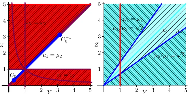
Fig. 1 Convergence regions in blue and divergence regions in red for classical Schwarz (left) and optimized Schwarz (right)
We now illustrate graphically the improvement of the optimized Schwarz method over the classical one in 2D. We show in Figure 1 in red the divergence regions and in blue the convergence regions for different values ofZandY. In the left graphic the white part is still an open problem. In the right the light blue line have convergence dependant of the mesh sizeh, the light blue region have convergence dependent on the coefficientsµ′sand the dark blue region have convergence independent of the
mesh sizehand the coefficientsµ′s, the red line is the zone of resonance corrected
with theorem 1. We clearly see that the optimization of the transmission conditions transforms an algorithm that fails for a large range of problems into one that works in all cases.
4 Conclusions
[image:8.612.138.464.93.257.2]8 Victorita Dolean, Martin J. Gander, Erwin Veneros
References
1. Alonso-Rodriguez, A., Gerardo-Giorda, L.: New nonoverlapping domain decomposition methods for the harmonic Maxwell system. SIAM J. Sci. Comput.28(1), 102–122 (2006) 2. Chevalier, P., Nataf, F.: An OO2 (Optimized Order 2) method for the Helmholtz and Maxwell
equations. In: 10th International Conference on Domain Decomposition Methods in Science and in Engineering, pp. 400–407. AMS (1997)
3. Despr´es, B.: D´ecomposition de domaine et probl`eme de Helmholtz. C.R. Acad. Sci. Paris
1(6), 313–316 (1990)
4. Despr´es, B., Joly, P., Roberts, J.: A domain decomposition method for the harmonic Maxwell equations. In: Iterative methods in linear algebra, pp. 475–484. North-Holland, Amsterdam (1992)
5. Dolean, V., El Bouajaji, M., Gander, M.J., Lanteri, S.: Optimized Schwarz methods for Maxwell’s equations with non-zero electric conductivity. In: Domain decomposition meth-ods in science and engineering XIX,Lect. Notes Comput. Sci. Eng., vol. 78, pp. 269–276. Springer, Heidelberg (2011).
6. Dolean, V., El Bouajaji, M., Gander, M.J., Lanteri, S., Perrussel, R.: Domain decomposition methods for electromagnetic wave propagation problems in heterogeneous media and complex domains. In: Domain decomposition methods in science and engineering XIX,Lect. Notes Comput. Sci. Eng., vol. 78, pp. 15–26. Springer, Heidelberg (2011).
7. Dolean, V., Gander, M.J., : Why Classical Schwarz Methods Applied to Hyperbolic Systems Can Converge even Without Overlap, In: Domain decomposition methods in science and engineering XVII,Lect. Notes Comput. Sci. Eng., vol. 60, pp. 467–475. Springer, Heidelberg (2007).
8. Dolean, V., Gerardo-Giorda, L., Gander, M.: Optimized Schwarz methods for Maxwell equa-tions. SIAM J. Scient. Comp.31(3), 2193–?2213 (2009)
9. Dolean, V., Lanteri, S., Perrussel, R.: A domain decomposition method for solving the three-dimensional time-harmonic Maxwell equations discretized by discontinuous Galerkin meth-ods. J. Comput. Phys.227(3), 2044–2072 (2008)
10. Dolean, V., Lanteri, S., Perrussel, R.: Optimized Schwarz algorithms for solving time-harmonic Maxwell’s equations discretized by a discontinuous Galerkin method. IEEE. Trans. Magn.44(6), 954–957 (2008)
11. Dubois, O.: Optimized Schwarz methods for the advection-diffusion equation and for prob-lems with discontinuous coefficients. Ph.D. thesis, McGill University (2007)
12. El Bouajaji, M., Dolean, V., Gander, M.J., Lanteri, S.: Optimized Schwarz methods for the time-harmonic Maxwell equations with damping. SIAM Journal on Scientific Computing
34(4), A2048–A2071 (2012).
13. Gander, M., Magoul`es, F., Nataf, F.: Optimized Schwarz methods without overlap for the Helmholtz equation. SIAM J. Sci. Comput.24(1), 38–60 (2002)
14. Gander, M.J.: Optimized Schwarz methods. SIAM J. Numer. Anal.44(2), 699–731 (2006) 15. Gander, M.J., Halpern, L., Magoul`es, F.: An optimized Schwarz method with two-sided robin
transmission conditions for the Helmholtz equation. Int. J. for Num. Meth. in Fluids55(2), 163–175 (2007)
16. Peng, Z., Lee, J.F.: Non-conformal domain decomposition method with second-order trans-mission conditions for time-harmonic electromagnetics. J. Comput. Physics229(16), 5615– 5629 (2010).
17. Peng, Z., Rawat, V., Lee, J.F.: One way domain decomposition method with second order transmission conditions for solving electromagnetic wave problems. J. Comput. Physics
229(4), 1181–1197 (2010).