Estimating an SME investment gap and the contribution of financing frictions ESRI WP589, March 2018

Working Paper 589

March

2018

a The Economic and Social Research Institute b Department of Economics, Trinity College Dublin

ESRI working papers are not ESRI reports. They represent un-refereed work-in-progress by researchers who are solely responsible for the content and any views expressed therein. Any comments on these papers will be welcome and should be sent to the author(s) by email. Papers may be downloaded for personal use only.

Estimating an SME investment gap and the contribution of financing

frictions

Martina Lawless

_{, Conor O'Toole}

_*

_and

_{Rachel Slaymaker}

Abstract: In this paper, we use firm-level survey data to explore the determinants of SME investment activity and the extent to which observed investment is in line with that suggested by economic fundamentals. In contrast to previous literature which has focused on whether investment gaps exist at a more aggregate level, we find evidence that for SMEs actual investment is below what would be expected given how companies are currently performing. The estimated magnitude of this investment gap is economically meaningful at just over 30 per cent in 2016. We explore the extent to which the gap is explained by financial market challenges such as access to finance, interest rates, and the availability of collateral. Financing frictions are found to account for a moderate share of the overall investment gap (between 10 per cent and 20 per cent of the gap).

*Corresponding Author: conor.otoole@esri.ie

Keywords: SMEs, financing constraints, investment, market failures

JEL Codes: O34, E01, D22, O38

1.

Introduction

Despite general economic recovery in the years following the financial crisis, concerns have been raised that investment levels have remained sluggish in many countries (Bussiere et al., 2015). This has raised questions whether this is due to poor economic fundamentals or whether the low levels of investment are due to structural factors such as credit constraints or other market failures preventing potentially productive investments being undertaken. The observation of low levels of investment is not sufficient to judge if there is under-investment in the economy overall or amongst specific groups of firms. Rather, the definition of an investment gap requires that investment be below a level in line with what should be expected by a firm’s performance and the cost of undertaking the investment. Döttling et al. (2017) found that the answer to this question varied across countries, with current investment profiles in Europe being well explained by economic fundamentals, whereas in the US there is evidence of an investment gap largely due to structural factors, including product market competition and a lessening of anti-trust enforcement.

Trying to separate the causes of weakness in investment growth into the demand-side factors and under-investment due to factors such as uncertainty, or the cost of financing is the central challenge in assessing if an investment gap exists. Bussiere et al (2015) used GDP forecasts at the time when investments took place to disentangle these factors, providing a forward-looking element to the estimation of their modelling of fundamental investment. They found that the cost of capital played a modest role in driving investment activity with nearly 80 per cent of the investment weakness, across the 22 countries they analysed, driven by economic fundamentals. A further 17 per cent was explained by the level of uncertainty. Their overall conclusion pointed to structural frictions such as financing constraints playing a modest role across the countries considered.

Other studies have found some evidence of investment gaps being related to credit conditions after the financial crisis, with Lewis et al (2014) estimating a gap for Germany, France and the United States between 2012 and 2014. As with Bussiere et al (2015), much of the investment shortfall in their study is also attributed to soft demand conditions, but with a not insubstantial role being attached to financial factors and heightened uncertainty. They note that recovery in investment could be boosted by tackling longer term structural issues such as financial fragmentation in the euro area and by implementing growth friendly structural reforms. Overall weakness in economic activity since the crisis began therefore appears as the primary constraint on business investment across most studies, with financial or other frictions playing a more minor part. Aggregate economic performance has a strong effect on investment, with the IMF (2014) estimating that a 1 per cent decline in output leads to a 2.4 per cent decline in investment.

The majority of the existing evidence on the presence and drivers of investment gaps across or within countries is macroeconomic in orientation and there are no studies to date which consider if there is an investment gap specifically for SMEs. This is despite the fact that SMEs have been found to be more likely to be affected by tightening of credit (e.g. Gerlach-Kristen et al. 2015), but this has not been linked to estimates of their fundamental levels of expected investment. This paper aims to fill this gap in the existing literature.

gap can be identified. Ireland is a particular interesting case study for this research given the challenge faced by SMEs following the financial crisis (Gerlach-Kristen et al., 2015; Lawless et al., 2015)

No previous study has focused on the SME sector and our results are substantially different from those found in studies of aggregate investment. We find evidence that current levels of firm investment are approximately 30 per cent lower than would be expected from the model based on fundamental factors in 2016. The size of the investment gap varies across groups of firms with the gap being considerably larger for medium-sized relative to micro or small enterprises.

We then examine the extent to which this investment gap can be explained by frictions in the availability of financing to firms. Although an investment gap is not solely caused by frictions in financing markets, considerable research has documented the impact of challenges in accessing finance on small firms generally (OECD, 2005), and in particular in Ireland since the onset of the financial crisis (O’Toole et al., 2014; Gerlach-Kristen et al., 2015; Holton et al., 2013). We find that financial frictions explain approximately 12-18 per cent of the gap. More specifically, we find investment is negatively related to the interest rate, credit rationing and borrower discouragement and increased where firms have been able to post tangible collateral such as cash, specific security over an asset or other collateral such as personal guarantees.

The paper is organised as follows: Section 2 discusses the economic intuition behind the investment gap and its determinants. Section 3 presents data and summary statistics and Section 4 presents the main empirical findings. Section 5 tests the robustness of the findings and Section 6 concludes.

2.

Measuring the Investment Gap

2.1 Determinants of firm investment

Economic models of firm behaviour mainly begin from the premise that there is a natural relationship between the capital inputs of a firm, its productive capacity and the output it produces. The motivation behind firms making new investment is to manage the relationship between the capital stock and output as firms grow. Many of the early papers modelling investment dynamics used so called accelerator models which linked investment to changes in output in a simple linear fashion (Jorgenson and Seibert, 1968).

More recently, standard neoclassical economic modelling of investment (Tobin, 1965; Chirinko, 1991) determined the optimal level of capital in an economy through the interaction between the marginal value product of capital (the extra return that a firm gains from adding one additional unit of investment) and the risk adjusted marginal cost of capital. Under this framework, we should see firms continuing to invest in capital until they no longer gain any extra revenue from more capital relative to its cost. These models assume perfect competition in input, output and capital markets.

will be lower than what would be optimal given the firms’ underlying profitability. An investment gap can therefore be defined as the difference between the unconstrained and the constrained level of investment.

2.2 Role of financial frictions

Although a number of structural rigidities and other factors can determine the size of an investment gap, particular focus has tended to be on the role played by financial frictions, particularly in the aftermath of the financial crisis. As is well documented in the literature (Berger and Udell, 1995), market failures occur in financial markets for a number of reasons. In the seminal Stiglitz and Weiss (1981) paper, they define credit rationing as the case whereby either a) identical firms receive different credit outcomes or b) some firms cannot access financing at any interest rate. In such cases where credit markets are failing to produce optimal, efficient outcomes, usually one of the following examples of market failures is at play (OECD, 2005):

• Moral hazard and principal agency problems – once funds have been allocated to borrowers, the incentives between the credit provider and the debtor can diverge. The credit provider has an incentive to ensure the borrower maximises the repayment likelihood whereas the debtor may look to take additional risks which maximise their expected return;

• Adverse credit selection – Banks or credit providers find it difficult to distinguish good risks from bad in cases with informational or communications deficits;

• Other monitoring difficulties - this may arise where the banks find it difficult to monitor the borrowers ex post performance, in particular where there is a blurring of the lines between the entrepreneurial venture and the household’s finances. Borrowers may also like to remain opaque to avoid tax or other regulatory burdens;

• Informational asymmetries – informational asymmetries relates to a broad range of market challenges whereby borrowers and lenders face different information sets when making decisions. In terms of applications for finance, these asymmetries normally arise where lenders do not have as good information about the firm as the owners or where the owners do not have well documented firm performance information. For example, these may arise where firms do not have a credit history or track record in repaying loans, haven’t been in business long enough to build up a performance history, or do not have experience in the sector or are just undertaking a new or innovative type of business activity, they may find it difficult to convince potential financers that they are not high risk; and

• Incomplete or unenforceable property and contract rights - in such circumstances, providers of finance may be less likely to allocate credit if they do not believe they can enforce the terms of the contract.

While these aforementioned market failures can exist for all firms, they are most likely to occur for SMEs, where corporate governance structures are not as strong as for larger firms, and where the information produced on the firm is more limited and transparency of the operations reduced (OECD, 2005; European Commission, 2014).

context, the fact that providing additional collateral can ease many of the burdens outlined above has led to partial credit guarantee schemes being an important component of the toolkit when addressing these issues from a public policy perspective (Honohan, 2010).

The aforementioned market failures can also be exacerbated by a number of structural features of the financial or banking markets in which the firms operate. In particular, if banks follow structurally restrictive credit practices such as blanket bans on lending to particular sectors, or if the risk tolerance of financial intermediaries is sufficiently adverse, this may lead to credit rationing. Furthermore, a lack of competition in financial services can lead banks to charge interest rates at above market levels which may cause many profitable investments to become unviable. A lack of competition can also lead to cases of credit rationing in selected sectors or markets.

2.3

Measuring the investment gap and its financing requirements in practice

Given the variety of potential determinants of an investment gap, one challenge that arises is to identify the most appropriate method with which to estimate the gap in practice. There are a number of methodologies that are commonly applied, some of which have been used to undertake recent empirical studies of the investment gap in Europe and the United States. Most of these models take a similar form, modelling investment as a function of indicators capturing the profitability or output growth of the firm and other control variables:

Investment = f(Measure of Fundamentals, Controls)

A model is then used to predict an investment figure given what would be expected for the level at which the firm is performing. The gap is then defined as the difference between the predicted values for investment and the actual data.

Gap = Actual - Predicted Investment

In terms of estimating the degree to which financial market frictions contribute to the slump in investment activity, existing studies use a range of different techniques. However, no research findings to date provide a clear or definitive methodology for how to do so. The most notable methodologies used to explore the extent to which the investment gap is due to financial factors come from the extensive literature on testing investment financing constraints by estimating how sensitive investment is to internal resources (Fazzari et al., 1988; Bond and Söderbom, 2013; O’Toole and Newman, 2017)1_{. Many of these studiesexplore whether investment is correlated}

with other proxies for potential market failures such as access to collateral. More recently, access to survey microdata has made the direct measurement of financing constraints possible from indicators of rejection rates and borrower discouragement. This has improved the accuracy with which the impact of financial market failures can be diagnosed. These financial factors are then appended to the econometric specification of the investment equation and their explanatory power tested:

Investment = f(Measure of Fundamentals, Financial Factors, Cost of Credit, Controls)

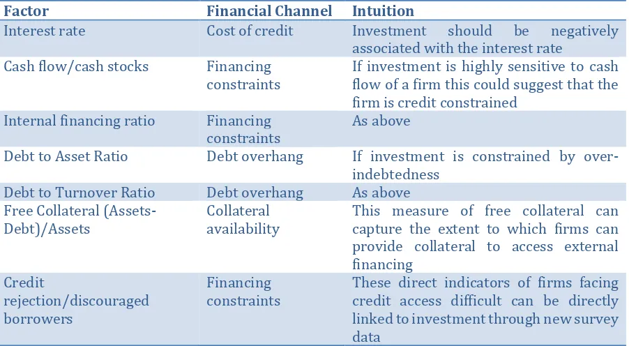
The inclusion of financial factors can be targeted to isolate which specific financial frictions are affecting investment. While a suite of potential financial factors have been used in the literature to address various aspects of financial market disfunction, the most common are presented in Table 1.

Table 1: Indicators of Financing Frictions

Factor Financial Channel Intuition

Interest rate Cost of credit Investment should be negatively

associated with the interest rate

Cash flow/cash stocks Financing

constraints If investment is highly sensitive to cash flow of a firm this could suggest that the

firm is credit constrained

Internal financing ratio Financing

constraints As above

Debt to Asset Ratio Debt overhang If investment is constrained by

over-indebtedness

Debt to Turnover Ratio Debt overhang As above

Free Collateral

(Assets-Debt)/Assets Collateral availability This measure of free collateral can capture the extent to which firms can

provide collateral to access external financing

Credit

rejection/discouraged borrowers

Financing

constraints These direct indicators of firms facing credit access difficult can be directly

linked to investment through new survey data

3.

Data and Methodology

3.1

Data source and summary statistics

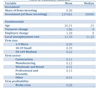
The firm level data comes from the SME Credit Demand Survey which is carried out on behalf of the Irish Department of Finance twice a year. We use eight waves of the survey, beginning with the period April-September 2013 up until the most recent wave relating to October 2016-March 2017. The survey captures a representative sample of SMEs in the Irish economy and is stratified by size and economic sector. A cross-section of approximately 1,500 firms is collected in each wave. Using eight waves, this gives us a total sample size of slightly over 12,000 firms. The survey provides a snapshot of SME performance and, in particular, the interactions of SMEs with the credit market both in terms of supply and demand of credit.

Summary statistics on the key variables of interest from the survey are presented in Table 2. Our central focus is on firm investment and in our econometric framework, we examine both the extensive and intensive margins of the investment decision. In this paper, we focus on fixed capital investment such as machinery, equipment, vehicles, plant and buildings. At the extensive margin, we find that on average 30 per cent of firms undertake some investment in each year and, of those investing, the average investment project is approximately €138,000. Investment amounts are highly skewed, with a small number of very large investments having a considerable effect on the mean amount. The median investment level per wave is €50,000.

percentage points.2

The mean response indicates firm growth for most of the sample over this timeframe, consistent with the overall recovery in the macroeconomy. A further measure of firm performance is an indicator of profitability, where three options were given to firms – made a profit (58 per cent of firms), broke even (28 per cent) or made a loss (14 per cent of firms). We also include dummy variables for if the firm is an exporter (expected to increase investment needs) and if they have previously defaulted on a loan (which we expect to limit investment both by increasing risk aversion and limiting financing). Including the default indicator also provides a direct control for firm credit risk.

We also control for the sector of the firm as there are likely to be differences, perhaps in the probability of investing, but more particularly in the scale of the average investment undertaken. Finally, to control for external demand factors, we include the unemployment rate for each wave of the region in which the firm is located (at the NUTS3 level).

Two main caveats should be noted with our research. First, as our data are cross-sectional, the estimated models with investment and economic fundamentals will suffer from simultaneity issues. This will likely lead to an over-estimate of the investment gap as coefficients are upward biased in the regressions. Second, most of our measures of financing constraints are binary variables and do not capture the quantum of any financing or collateral gap at a firm level. Better monetary measures of the demand for finance at the firm level would improve our modelling accuracy. This will likely bias downwards any explanation for how much financing factors explain the investment gap. Improving these two data limitations would greater enhance the accuracy of the estimates.

Table 2: Summary Statistics

Variable Mean Median

Investment

Share of firms investing _{0.30 .}

Investment (of those investing) _{137681 50000}

Fundamentals

Age _{26.31 21}

Turnover change _{1.86 0}

Employee change _{1.28 0}

Local unemployment rate _{11.39 11.25}

Firm size:

1-9 Micro _{0.39 .}

10-49 Small _{0.39 .}

50-249 Medium _{0.22 .}

Firm sector:

Construction _{0.11 .}

Manufacturing _{0.12 .}

Wholesale and Retail _{0.31 .}

Professional and

Scientific 0.15 .

Other _{0.31 .}

Firm profitability:

Broke even _{0.28 .}

Profit _{0.58 .}

Loss _{0.14 .}

Default _{0.04 .}

Export _{0.21 .}

Number of observations _{12,091 12,091}

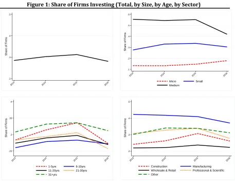
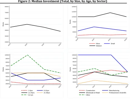
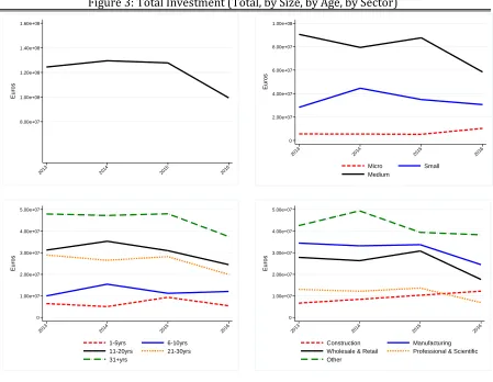
Figures 1, 2 and 3 show how firm investment patterns differ for the overall sample and also by firm size, age and sector of activity. Figure 1 shows the probability of investing (i.e. the share of each group of firms with positive investment in each year). Figure 2 graphs the median investment amount and Figure 3 shows how each firm type contributes to total investment.

In addition to the fall in investment shares in 2016, overall median investment amounts also declined between 2014 and 2016 as shown in the top-left of Figure 2. The median amount fell from €50,000 to just under €40,000. The reduction in the share of firms investing, together with lower median investment result in a reduction in total investment amongst the surveyed firms in 2016, shown in the top-left quadrant of Figure 3. The pattern across firm size groups for median investment amounts is very similar to that of investment participation, with the medium-sized firms investing larger amounts as well as being more likely to invest. Similarly, the oldest firms in the sample invest the highest median amounts as well as being the most likely to invest. Conversely, however, the youngest firms have very low median investments – less than half of the overall median - despite being the second most likely of the age groups to undertake some investment. The reduction in total investment at the end of the sample period correlates quite strongly at this descriptive level, with a large reduction in median investment amounts by manufacturing firms, which in previous periods had been the largest median investors by a considerable margin.

Figure 1: Share of Firms Investing (Total, by Size, by Age, by Sector)

Source: ESRI Analysis of CDS Data .2 .3 .4 .5 Sh a re o f F irms

2013 2014 2015 2016

.1 .2 .3 .4 .5 .6 Sh a re o f F irms

2013 2014 2015 2016

Micro Small Medium .25 .3 .35 .4 Sh a re o f F irms

2013 2014 2015 2016

1-5yrs 6-10yrs 11-20yrs 21-30yrs 31+yrs .2 .3 .4 .5 Sh a re o f F irms

2013 2014 2015 2016

Figure 2: Median Investment (Total, by Size, by Age, by Sector)

Source: ESRI Analysis of CDS Data 20000

30000 40000 50000 60000 70000 80000

Eu

ro

s

2013 2014 2015 2016

0 25000 50000 75000 100000 125000 150000

Eu

ro

s

2013 2014 2015 2016

Micro Small Medium

20000 30000 40000 50000 60000 70000 80000 90000 100000

Eu

ro

s

2013 2014 2015 2016

1-5yrs 6-10yrs 11-20yrs 21-30yrs 31+yrs

20000 30000 40000 50000 60000 70000 80000 90000 100000

Eu

ro

s

2013 2014 2015 2016

Figure 3: Total Investment (Total, by Size, by Age, by Sector)

Source: ESRI Analysis of CDS Data

3.2 Investment Gap Estimation Method

In order to estimate the size of the investment gap, the first step is to establish a fundamental level of investment that firms with different characteristics would be expected to undertake. We then take the predicted values of the fundamental level of investment from the model and compare these to the actual investment amounts. The difference between the firm’s actual investment and the predicted fundamental level gives us a measure of under- (or over-) investment. The fundamental investment and size of the investment gaps can then be aggregated to examine how they vary across different groups of firms.

The model used to estimate the fundamental level of investment is a two-stage Heckman specification. This separates the investment decision at the firm level into two components – first, the choice is made to undertake an investment project or not and, second, if the firm decides that it wants to invest it then decides on the size of the investment. An attractive feature of this approach is that it allows for firm characteristics to have differential effects on the two components of the investment decision process; for example, we saw in the summary statistics that young firms are amongst the most likely to invest but then have the lowest median investment scale.

The first stage of the Heckman specification is a probit regression where the dependent variable

Prob_Investit is a dummy variable with a value of 1 if the firm i has positive investment in period

8.00e+07 1.00e+08 1.20e+08 1.40e+08 1.60e+08 Eu ro s

2013 2014 2015 2016

0 2.00e+07 4.00e+07 6.00e+07 8.00e+07 1.00e+08 Eu ro s

2013 2014 2015 2016

Micro Small Medium 0 1.00e+07 2.00e+07 3.00e+07 4.00e+07 5.00e+07 Eu ro s

2013 2014 2015 2016

1-5yrs 6-10yrs 11-20yrs 21-30yrs 31+yrs 0 1.00e+07 2.00e+07 3.00e+07 4.00e+07 5.00e+07 Eu ro s

2013 2014 2015 2016

t and zero if there is no investment.

𝑃𝑃𝑃𝑃𝑃𝑃𝑃𝑃_𝐼𝐼𝐼𝐼𝐼𝐼𝐼𝐼𝐼𝐼𝐼𝐼𝑖𝑖𝑖𝑖 =�1 ₀ 𝑖𝑖𝑖𝑖_{𝑖𝑖𝑖𝑖}𝐼𝐼𝐼𝐼𝐼𝐼𝐼𝐼𝐼𝐼𝐼𝐼_{𝐼𝐼𝐼𝐼𝐼𝐼𝐼𝐼𝐼𝐼𝐼𝐼}> 0_{= 0}

This is regressed on a set of firm characteristics Xit including size, age, changes in turnover and

employees, as well as indicators of profitability, export status and previous loan default. We also include a number of control variables to capture effects of time (survey wave indicators), region and sector. The regional unemployment rate is also included to capture different trends in local demand conditions.

𝑃𝑃𝑃𝑃𝑃𝑃𝑃𝑃_𝐼𝐼𝐼𝐼𝐼𝐼𝐼𝐼𝐼𝐼𝐼𝐼𝑖𝑖𝑖𝑖 =𝛼𝛼+𝛽𝛽1𝑋𝑋𝑖𝑖𝑖𝑖+𝛽𝛽2𝐶𝐶𝑃𝑃𝐼𝐼𝐼𝐼𝑃𝑃𝑃𝑃𝐶𝐶𝐼𝐼+𝜀𝜀𝑖𝑖𝑖𝑖

The second stage then models the investment level, using the same set of explanatory variables as used in the investment decision equation.

𝐿𝐿𝐼𝐼(𝐼𝐼𝐼𝐼𝐼𝐼𝐼𝐼𝐼𝐼𝐼𝐼𝑖𝑖𝑖𝑖) =𝛼𝛼+𝛽𝛽1𝑋𝑋𝑖𝑖𝑖𝑖+𝛽𝛽2𝐶𝐶𝑃𝑃𝐼𝐼𝐼𝐼𝑃𝑃𝑃𝑃𝐶𝐶𝐼𝐼+𝜇𝜇𝑖𝑖𝑖𝑖

4.

Results for the Investment Gap and Financing Contribution

4.1 Fundamental and Actual Investment

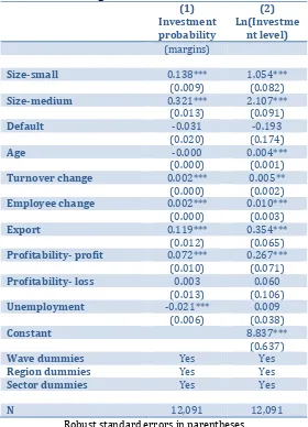
The results from the Heckman model showing the determinants of the investment choice and scale in the model of fundamental investment are presented in Table 3. Column 1 shows the results from the first stage (the decision to invest or not) and Column 2 shows the determinants of investment amounts. Controlling for other factors, we find confirmation of a strong positive relationship between firm size and both the probability of investment and the volume. Have previously defaulted on a loan, although it has a negative coefficient, is not a statistically significant factor in either investment decisions or levels. The firm’s age does not have any correlation with the probability of making an investment, but we do find that older firms tend to invest more.3

The measures of firm performance (changes in employment, turnover, profitability and being an exporter) all have the expected positive relationships with both investment probability and size of investment. Regional unemployment affects the two decision margins differently, having a statistically significant negative effect on the probability of undertaking investment, but no correlation with the size of an investment.

3 _{In an alternative specification we also included an age squared term to account for a potential non-linearities;}

Table 3: Regression Model - Fundamentals (1)

Investment probability

(2) Ln(Investme

nt level)

(margins)

Size-small 0.138*** 1.054***

(0.009) (0.082)

Size-medium 0.321*** 2.107***

(0.013) (0.091)

Default -0.031 -0.193

(0.020) (0.174)

Age -0.000 0.004***

(0.000) (0.001)

Turnover change 0.002*** 0.005**

(0.000) (0.002)

Employee change 0.002*** 0.010***

(0.000) (0.003)

Export 0.119*** 0.354***

(0.012) (0.065)

Profitability- profit 0.072*** 0.267***

(0.010) (0.071)

Profitability- loss 0.003 0.060

(0.013) (0.106)

Unemployment -0.021*** 0.009

(0.006) (0.038)

Constant 8.837***

(0.637)

Wave dummies Yes Yes

Region dummies Yes Yes

Sector dummies Yes Yes

N 12,091 12,091

Robust standard errors in parentheses *** p<0.01, ** p<0.05, * p<0.1

Figure 4: Actual SME Investment and Model Prediction by Year

Source: ESRI Analysis of CDS Data

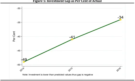
Figure 5: Investment Gap as Per Cent of Actual

4.2 How much of the gap is due to financial market failures?

An important consideration in order to understand enterprise behaviour, as well as to understand the policy implications of the evident under-investment, is to determine what factors are determining the investment gap. The existing literature, discussed in Section 2, points to a range of factors influencing firm behaviour, with uncertainty, financing constraints and market competition as notable influences in the US and Europe since the global financial crisis.

In this paper, our focus is on understanding the extent to which financial market imperfections are a determining factor in the degree of under-investment in Ireland. Given the scale of the banking crisis in Ireland, and the existing research that highlights the impact of credit constraints on SME investment since the crisis (Gerlach-Kristen et al., 2015), our a-priori expectations would be that some of this gap may be caused by disruptions to the intermediation of finance. However, a direct test of whether or not this is the case can provide more insight as well as providing, in an ex-ante sense, evidence as to which policy instruments could be deployed to help reduce the investment gap.

In general, the literature on the impact of financing constraints on investment mainly attempts to address this issue by including proxies for the degree of constraints in investment equations and by then testing whether or not they have an economic impact on the firm’s capital expenditure. In our analysis we follow this approach as our baseline test and we document it in detail below. The standard approach to testing the impact of financial market frictions on investment in the academic literature is to include proxy variables for credit access challenges into the investment specification and to test whether or not they are economically significant. As we are interested in understanding the extent to which these factors explain the investment gap, we need to go a step further and explore how they affect our model prediction for investment.

However, our first step is to obtain a number of proxies for financial market imperfections that could be included in our model. Given its rich insight into the financial behaviour of firms and their indebtedness, the Department of Finance Credit Demand Survey provides a number of different indicators that we can use. Our aim is to approximate a number of channels of financial market failures with direct indicators in the model. The variables selected are presented in Table 5 with their measurement and the rationale behind them. The inclusion of these variables is based on a combination of data availability and the existing literature.

The definition of each variable is provided in Table 13 in the appendix. We include the interest rate that the firms currently pay on their outstanding debt to approximate the cost of capital. For those firms who do not have debt outstanding, we include an interest rate which is the average for a similar firm in terms of age, size, sector, and time period. This approximation should attempt to capture the fact that firms, aware of what prevailing interest rates are, could change their investment patterns.

Table 5: Financing Frictions Variables

Interest rate Cost of financing Higher interest rates should lower investment

Credit access Applications for

finance and their success

We split the sample into borrowers who had successfully applied for credit, rejected borrowers, discouraged borrowers and those that did not apply. Investment should be higher for successful applicants.

Lending conditions Access to, demand

for, finance We include a variable for whether or not firms believe the banks are lending. If this lowers credit demand, it should have a negative association with investment.

No collateral

posted Access to finance We distinguish between those firms who applied for financing and posted specific collateral and all other firms as a proxy for the collateral channel.

Debt to turnover

ratio Debt overhang This indicator reflects the degree to which debt sustainability impacts investment.

Total debt Indebtedness This measure of free collateral can capture the extent to

which firms can provide collateral to access external financing.

To measure credit access directly, we use two variables. First, we include indicators for firms who were denied credit (credit rejected), firms who were discouraged from applying, and firms who did not apply. This should capture differences in the relative demand for financing, as well as stripping out supply side constraints from rejections and discouragement. As discouraged borrowers have been found to lower investment and employment levels for SMEs (Gerlach-Kristen et al., 2015), we also augment our regression with a variable measuring how firms view bank lending conditions. More specifically, we control for whether or not the firm believes the banks are lending to SMEs.

A well-documented symptom of financial market failures is a lack of collateral being posted by firms. If firms do not have sufficient collateral to compensate financial institutions for assessed risk, this can limit their ability to access credit and subsequently invest. A lack of collateral is also a clearly defined area in which public policy, through the use of risk sharing initiatives or guarantee facilities (Honohan, 2010), can intervene to help the flow of finance. Previous research for Ireland clearly shows that collateralisation is used to manage risk ex-ante, in particular for very large loans (Carroll and McCann, 2017), and that personal guarantees were a very prevalent collateral type in Ireland (Carroll et al., 2015). Ideally, to measure the collateral channel, the researcher would have a measure for the total net worth of the company including cash holdings, physical or intangible assets and inventories that could be posted to secure loans. In our survey, we do not have such a measure. However in attempting to control for the collateral channel as best as possible, we distinguish those firms who posted collateral when applying for credit relative to all other firms. If we find these firms have higher investment, controlling for other factors including the credit access of the firm, this can provide insight into the existence of a collateral channel.

Two final factors that we include are motivated by Lawless et al. (2015) and attempt to capture debt overhang channels. We include the size of debt outstanding and the debt-to-turnover ratio which can capture two aspects: 1) debt sustainability and 2) it may pick up some collateral effects (as firms with high levels of debt relative to their turnover may have low levels of collateral). Summary statistics for all of these factors are contained in Table 6 below:

Table 6: Summary Statistics – Financial Frictions

Financial frictions

Interest rate 5.68 5.42

DTI lag 0.21 0.01

lnD lag 6.36 8.70

No collateral posted 0.91 .

Tight lending conditions 0.27 .

Credit access:

Successful _0.22 .

Rejected _0.05 .

Discouraged borrowers _0.06 .

Did not apply _0.67 .

N _{11,094 11,094}

In terms of our econometric methodology, we append the financial variables to the baseline specification for the economic fundamentals across both the investment decision stage and the investment level stage. This allows each of the variables to have a separate influence on these two parts of a firm’s investment activity. The findings are presented in Table 7 below. In the investment decision regression, we find that the likelihood of investment is falling in credit rejection, borrower discouragement and firm’s views on the tightness of lending conditions. Investment is also negatively associated with the debt to turnover indicator, suggesting increased indebtedness lowers investment. We also find a negative relationship with the interest rate, indicating that the level of interest rates is lowering investment decisions. In this regression, we find that collateral has no effect on the investment decision.

In terms of the levels regression, we find that investment is materially lower for firms who did not post collateral when borrowing, as well as for discouraged borrowers and firms with no credit applications. We do not find an impact of the debt-to-turnover ratio or the interest rate in this stage of the decision making. It is not necessarily surprising that these influences are lessened in the level estimation as, with only 30 per cent of firms investing in any one six month period, the number of firms with positive levels of investment is low which compromises the ability of the model to determine the effects. More generally, the two parts of the investment equation capture the firm’s behaviour jointly so the findings should be interpreted as such i.e. if a variable has an influence on either stage, we can conclude it is important for firms’ decision making.

It is important to draw out some of the limitations of our approach at this point. All of our regressions are conducted on a repeated cross-sectional dataset. As we do not observe the firms over time, we cannot understand how their individual behaviour is changing over time. Furthermore, as most of the variables (excluding debt) are contemporaneous to the investment variables, the relationship is endogenous i.e. investment activity will impact turnover growth and employment growth as well as these being explanatory factors for investment. This will lead to some bias in the estimates which may potentially affect the coefficients estimated. On balance, it is likely the bias is positive and overstates certain relationships. This is also the case for our credit access indicators.

Table 7: Regression Model – Financial Frictions

(1) (2)

(Yes, No) (in Logs)

No collateral posted -0.013 -0.219**

(0.018) (0.097)

Credit access - rejected -0.071*** 0.124

(0.023) (0.137)

Credit access - discouraged borrower -0.072*** -0.352**

(0.022) (0.163)

Credit access – did not apply -0.066*** -0.213***

(0.013) (0.074)

Tight lending conditions -0.027*** -0.025

(0.010) (0.068)

DTI lag -0.023*** 0.032

(0.009) (0.050)

lnD lag 0.005*** 0.016***

(0.001) (0.005)

Interest rate -0.005*** 0.000

(0.002) (0.010)

Constant 9.289***

(0.645)

Wave dummies Yes Yes

Region dummies Yes Yes

Sector dummies Yes Yes

Fundamental Factors Yes Yes

N 11,094 11,094

Robust standard errors in parentheses *** p<0.01, ** p<0.05, * p<0.1

Having estimated the regression model, we now turn to exploring the impact of financial factors on the investment gap. We begin with the economic fundamentals model documented in section 4.1 above. When we estimate this model, and then use it to predict a level of investment, the component of investment that might be explained by financial factors is left in the error term. When we append financial variables to the model, the component explained by these variables comes out of the error term and into the prediction. Our approach to identifying the financing share of the gap is to then compare the predicted value from the fundamentals model to the predicted value of the model with financial frictions. We provide two comparisons as follows:

𝐹𝐹𝑖𝑖𝐼𝐼𝐹𝐹𝐼𝐼𝐹𝐹𝑖𝑖𝐼𝐼𝐹𝐹𝐺𝐺𝐹𝐹𝐺𝐺 (𝑀𝑀𝐼𝐼𝐹𝐹𝐼𝐼) = �𝑀𝑀𝐼𝐼𝐹𝐹𝐼𝐼𝐼𝐼𝐸𝐸𝐸𝐸𝐸𝐸𝐸𝐸𝐸𝐸𝐸𝐸𝑖𝑖𝐸𝐸𝑃𝑃_{𝑀𝑀𝐼𝐼𝐹𝐹𝐼𝐼𝐼𝐼}− 𝑀𝑀𝐼𝐼𝐹𝐹𝐼𝐼𝐼𝐼𝐶𝐶𝐶𝐶𝐶𝐶𝐶𝐶𝑖𝑖𝑖𝑖𝑃𝑃 �

𝐸𝐸𝐸𝐸𝐸𝐸𝐸𝐸𝐸𝐸𝐸𝐸𝑖𝑖𝐸𝐸𝑃𝑃 𝑥𝑥 100

Where 𝑀𝑀𝐼𝐼𝐹𝐹𝐼𝐼𝐼𝐼𝐸𝐸𝐸𝐸𝐸𝐸𝐸𝐸𝐸𝐸𝐸𝐸𝑖𝑖𝐸𝐸𝑃𝑃 takes the predicted value of the economic fundamentals model and sums

it across all firms and 𝑀𝑀𝐼𝐼𝐹𝐹𝐼𝐼𝐼𝐼𝐶𝐶𝐶𝐶𝐶𝐶𝐶𝐶𝑖𝑖𝑖𝑖𝑃𝑃 takes the predicted value of the model with financial and credit

variables in the model and sums it across all companies. The superscript p denotes a model prediction. We then take the difference between these predicted values as a percentage of the economic fundamentals model to understand how much the gap changes when financial frictions are included.

large investments, using the median captures the “middle” firm in the distribution. When a distribution has a large right tail like investment, the median is a better measure of the(?) central tendency. The formula for the gap then becomes:

𝐹𝐹𝑖𝑖𝐼𝐼𝐹𝐹𝐼𝐼𝐹𝐹𝑖𝑖𝐼𝐼𝐹𝐹𝐺𝐺𝐹𝐹𝐺𝐺 (𝑀𝑀𝐼𝐼𝑀𝑀) = �𝑀𝑀𝐼𝐼𝑀𝑀𝐼𝐼𝐸𝐸𝐸𝐸𝐸𝐸𝐸𝐸𝐸𝐸𝐸𝐸𝑖𝑖𝐸𝐸𝑃𝑃_{𝑀𝑀𝐼𝐼𝑀𝑀𝐼𝐼} − 𝑀𝑀𝐼𝐼𝑀𝑀𝐼𝐼𝐶𝐶𝐶𝐶𝐶𝐶𝐶𝐶𝑖𝑖𝑖𝑖𝑃𝑃 �

𝐸𝐸𝐸𝐸𝐸𝐸𝐸𝐸𝐸𝐸𝐸𝐸𝑖𝑖𝐸𝐸𝑃𝑃 𝑥𝑥 100

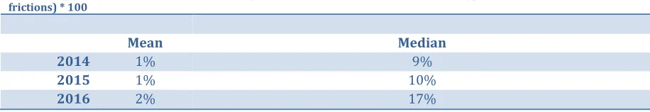
Where Med I denotes the median investment for the fundamentals (economic) and financial (credit) models. The estimates of the financing gap from our econometric model are presented in Table 8 below by year. Given the effects on the calculation of the larger investments, our preferred estimate is based on the median.

Table 8: Model Based Estimates of Financing Frictions

Method - (predicted model without frictions - predicted value from model with frictions/predicted model without frictions) * 100

Mean Median

2014 1% 9%

2015 1% 10%

2016 2% 17%

One further limitation to highlight at this juncture relates to the predictive power of a model such as ours with a large number of binary indicators as proxies for financing constraints. These variables approximate an underlying continuous amount of financing that firms are unable to access. If we only approximate this with a variable that is one or zero, the prediction from the model then just adds an intercept adjustment. This effect is confounded by the fact that many of our indicators have a large number of zero values as firms don’t apply for credit and therefore do not indicate whether they would post collateral. This reduces the ability of the model to provide differences across firms and limits the extent to which it explains the variation in the continuous investment variable.

4.3 Exploring differences across firms

To provide some insight into whether there are differences across firms in the extent of the under-investment patterns, we present estimates for the under-investment gap by firm sector, size and age group. We also present an estimate of the extent to which financing was playing a role in the under-investment. It must be noted that when these estimates are disaggregated to such an extent they can become very volatile. Given this consideration, we calculate the gaps over the entire 2014-2016 period in an attempt to provide more stability.4

The differences across sectors are presented in the Table 9 below. It can be seen that the largest gaps are in the wholesale and retail sector, manufacturing, and construction and real estate. In terms of the share of the gap attributable to financing frictions, the highest is the wholesale and retail sector.

Table 9: Estimates of Investment Gap by Sector

SECTOR Gap (As Percent of Actual) Financing Share of Gap (median)

4 _{We also estimated our model on separate subsamples across sectors and size classes. However, we do not}

Cons & RE -54% 8%

Manu _-64% 8%

W&R -41% 12%

Prof&Scie -31% 9%

Other -26% 5%

The estimates across firm size are presented in Table 10. It can be seen that the greatest share of under-investment is taking place amongst the largest firms. The model in fact indicates that micro sized firms are actually over-investing relative to their fundamentals. This can however be explained by the fact that the model predicts very small investments for this class of firm, whereas in reality, many of these companies invest quite large amounts relative to this size. When the figures are summed over all companies, the large positive investments outweigh the smaller predictions. We also document that micro investment could actually increase by a further 11 per cent if financing constraints were lowered. These findings can be reconciled by the fact that the very small constrained micro firms are still under-investing while some other non-constrained micro firms are investing strongly.

Table 10: Estimates of Investment Gap by Size

SIZE Gap (As Percent of Actual) Financing Share of Gap (median)

Micro 2% .

Small -25% 5%

Medium -54% 6%

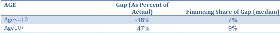
The estimated investment gap by firm age is presented in Table 11 below. Under-investment appears highest in the older firms in Ireland, and these firms also face a higher share of financing constraints.

Table 11: Estimates of Investment Gap by Age

AGE Gap (As Percent of

Actual) Financing Share of Gap (median)

Age<=10 -16% 7%

Age10+ -47% 9%

5.

Robustness Checks

To examine the robustness of our findings, we also apply an alternative methodology that follows the ex-ante guidelines outlined by the European Investment Fund in their 2014 publication for SME financial market assessments (Lang and Kramer-Eis, 2014). In these guidelines, they provide a rough estimate of the loan-financing gap, giving a formula that can be applied to survey data. It takes into account firm performance, credit constraints in the economy and the average loan demand. They define the financing gap as:

Loan Financing Gap = No. Firms x Credit Risk x Credit Access x Average Loan Size

This estimate provides a quantum for the total level of credit undersupplied to the market, without the requirement to undertake a detailed supply and demand assessment in a modelling framework. Given that it uses credit access (credit rejected and discouraged borrowers) information as well as information on credit risk, it goes some way to capturing the supply and demand side factors using a micro data foundation.

then calibrate the estimate to take into account the investment orientation of credit demand by adjusting our estimate by the share of borrowers who applied for investment oriented credit using the Credit Demand Survey. Like investment, our loan application data is highly skewed with some very large loans. We therefore use the median loan application size from the Credit Demand Survey as our representative loan size. We define credit constrained borrowers as both rejected and discouraged. The formula we apply is therefore:

Financing Gap Per Firm = (No. Firms x Non-Default x Non-Loss Making x Credit Constrained x Investment Focus of Loan Demand x Representative Loan Size)/No. Firms

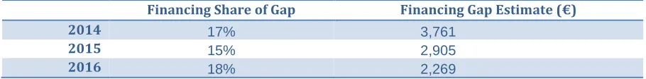
The financing loan gap that is estimated from the formula above is then presented as a share of the total investment gap from the model and the figures are presented in Table 12. The results are similar in magnitude to those we estimate in our model-based approach, particularly for 2016 but are higher in earlier years. Overall, this method displays less variation over time compared to the model-based estimation which is perhaps unsurprising given that more aggregate figures may smooth over the volatilities in the firm-level assessment.

Table 12: EIF Financing Gap Assessment

Financing Share of Gap Financing Gap Estimate (€)

2014 17% 3,761

2015 15% 2,905

2016 18% 2,269

6.

Conclusions

Since the onset of the global financial crisis, fixed capital formation growth internationally has been muted, with developments in the Irish market typical of many countries. While existing research suggests that the lagging recovery investment levels were more to do with uncertainty and muted growth prospects, there is some evidence that suggests difficulties in financial markets have led to firms missing profitable opportunities. This is particularly so in countries where the effects of the financial crisis were hardest felt (Phillipon et al., 2017; Bussiere et al., 2015). Ireland falls into this latter category with existing studies slowing credit access and debt overhang curtailed investment (Gerlach-Kristen et al., 2015; Lawless et al., 2015).

In this paper, we build on the existing research to explore whether the investment activity of Irish SMEs is in line with their economic fundamentals. Using micro data at the firm level, we determine investment as a function of firm’s turnover growth, employment growth, profitability, exporting status, age, credit risk, and local economic conditions. We find evidence that actual investment is below what would be expected given how companies are currently performing. The magnitude of this “investment gap” is economically meaningful and is estimated to be just over 30 per cent in 2016. Given that our data are cross-sectional, we are not able to causally determine the relationships between investment and fundamentals. This will likely cause a positive bias in the estimates and make our findings on the gap an upper bound i.e. with a longitudinal dataset, it is likely the gap would be lower. We find the gap is greatest for medium-sized firms and older firms.

There are a number of specific policy implications that arise from our research. First, we document that Irish firms are under-investing and the magnitude of this under-investment is larger than shown in previous research which uses country level data. We also find that up to 18 per cent of this is due to financial market failures. While this leaves a majority of the gap unexplained, it does provide clear evidence that addressing credit market difficulties will raise investment and increase economic activity. We find the cost of capital is negatively related to investment. As documented in McQuinn et al. (2017) the cost of credit for business is high in Ireland and previous research has shown that interest rates are higher in Ireland than what would be expected based on observed firm risk (Carroll and McCann, 2017).

References

Berger, A.N., and G.F. Udell (1995). ‘Relationship lending and lines of credit in small firm finance’,

Journal of Business, Vol. 68, No. 3, pp.351-381.

Bond, S.R., and M. Söderbom (2013). ‘Conditional investment–cash flow sensitivities and financing constraints’, Journal of the European Economic Association, Vol. 11, No. 1, pp.112-136.

Bussiere, M., L. Ferrara, and J. Milovich (2015). ‘Explaining the Recent Slump in Investment: the Role of Expected Demand and Uncertainty’, Banque de France Document de Travail No. 571.

Carroll, J. and McCann, F. (2017), `Observables and residuals: exploring cross border differences in SME borrowing costs’, Research Technical Papers, Central Bank of Ireland.

Carroll, J., F. McCann, and C. O'Toole (2015). ‘The use of personal guarantees in Irish SME lending’, Economic Letters, Dublin: Central Bank of Ireland.

Carroll, J., and F. McCann (2017). ‘SME Collateral: risky borrowers or risky behaviour?’ Central Bank of Ireland Research Technical Paper 06RT17.

Chirinko, R.S., (1993). ‘Business fixed investment spending: Modelling strategies, empirical results and policy implications’, Journal of Economic Literature, 31, 1875-1911.

Döttling, R., G. Gutiérrez, and T. Philippon (2017). ‘Is there an investment gap in advanced economies? If so, why?’

European Commission (2014) ‘Ex-ante assessment methodology for financial instruments in the 2014-2020 programming period’, Volume 1, Brussels.

European Investment Bank (2017) ‘Investment and Investment Finance in the EU: 2016’, Annual Report, Luxembourg.

Fazzari, S. M., R.G. Hubbard, and B.C. Petersen (1988). ‘Financing constraints and corporate investment’, Brookings Papers on Economic Activity, Vol. 19, No. 1, pp. 141–206.

Gerlach-Kristen, P., B. O'Connell, and C. O'Toole (2015). ‘Do credit constraints affect SME investment and employment?’, The Economic and Social Review, Vol. 46, No. 1, pp.51-86. Holton, S., M. Lawless, and F. McCann (2013). ‘SME financing conditions in Europe: credit crunch

or fundamentals?’, National Institute Economic Review, Vol. 225, No. 1, pp.R52-R67. Honohan, P., (2010) ‘Partial credit guarantees: principles and practice’, Journal of Financial

Stability, Vol 6, (1), pp.1-9.

IMF (2014), World Economic Outlook, April, Washington D.C.

Jorgenson, D.W., and C.D, Siebert (1968). ‘A comparison of alternative theories of corporate investment behavior’, The American Economic Review, Vol. 58, No. 4, pp.681-712.

Kramer-Eis, H. and Lang, F., (2014) ‘Guidelines for SME Access to Finance Market Assessments’, Working Paper 2014/22, European Investment Fund.

Lawless, M., B. O’Connell, and C. O’Toole (2015). ‘SME recovery following a financial crisis: Does debt overhang matter?’ Journal of Financial Stability, Vol. 19, pp.45-59.

Lewis, C., N. Pain, J. Stráský, and F. Menkyna (2014). ‘Investment Gaps after the Crisis’, OECD Economics Department Working Papers, No. 1168, OECD Publishing, Paris.

McQuinn, K., D. Foley, and C. O'Toole (2017). ‘Quarterly Economic Commentary, Summer 2017,’ Forecasting Report, Economic and Social Research Institute (ESRI), number QEC20172, April.

OECD (2005) ‘The SME Financing Gap: Volume 1”, Paris.

O'Toole, C.M., C. Newman, and T. Hennessy (2014). ‘Financing constraints and agricultural investment: Effects of the Irish financial crisis’ Journal of Agricultural Economics, Vol. 65, No. 1, pp.152-176.

O’Toole, C., and C. Newman (2017). ‘Investment Financing and Financial Development: Evidence from Viet Nam’, Review of Finance, Vol. 21, No. 4, pp.1639-1674.

Ryan, R., O’Toole, C. and McCann, F. (2014) ‘Does bank market power affect SME credit constraints?’, Journal of Banking and Finance, 49(c), pp.495-505.

Stiglitz, J.E. and A. Weiss (1981). ‘Credit rationing in markets with imperfect information’, The

Appendix

Table 13: Variable Definitions

Variable Definition

Region NUTS3 region:

Border (base group) Dublin

Mid-East Mid-West Midlands South-East South-West West

Sector Firm sector:

Construction (base group) Manufacturing

Wholesale and Retail Hotels and Restaurants Professional and Scientific Other

Size Categorical variable representing firm size in terms of

number of employees:

1-9 Micro (base group) 10-49 Small

50-249 Medium

Age Age of the firm

Employee growth Percentage change in the number of employees at the firm in

the last 6 months

Turnover growth Percentage change in firm turnover in the last 6 months

Local unemployment rate Unemployment rate in the NUTS 3 region in which the firm is

located

Profitability Categorical variable representing firm profitability in the last

6 months:

0 Broke even (base group) 1 Profit

2 Loss

Export Binary variable =1 if the firm exports and =0 otherwise

Default Binary variable =1 if the firm has defaulted on any loan

repayments in the last 6 months and =0 otherwise

Credit access Categorical variable representing a firm’s ease of access to

credit:

0 Successfully accessed finance (base group) 1 Rejected

2 Discouraged borrower 3 Did not apply

lnD lag Log of lagged total debt

Lending conditions Binary variable =1 if the firm believes lending conditions are tight (banks are not lending or are only lending to a small number of SMEs) and =0 otherwise

No collateral posted Binary variable =1 if the firm has not put up collateral

(personal guarantee, specific security, cash or additional collateral) and =0 otherwise

Interest rate Either the interest rate faced by the firm if they report it or

Year

Number

Title/Author(s)

588 Supporting decision-making in retirement planning: Do diagrams on pension benefit statements help?

Pete Lunn and Féidhlim McGowan

587 Productivity spillovers from multinational activity to indigenous firms in Ireland

Mattia Di Ubaldo, Martina Lawless and Iulia Siedschlag

586 Do consumers understand PCP car finance? An experimental investigation

Terry McElvaney, Pete Lunn, Féidhlim McGowan

585 Analysing long-term interactions between demand response and different electricity markets using a stochastic market equilibrium model

Valentin Bertsch , Mel Devine , Conor Sweeney , Andrew C. Parnell

584 Old firms and new products: Does experience increase survival?

Martina Lawless and Zuzanna Studnicka

583 Drivers of people's preferences for spatial proximity to energy infrastructure technologies: a cross-country analysis

Jason Harold, Valentin Bertsch, Thomas Lawrence and Magie Hall

582 Credit conditions and tenure choice: A cross-country examination

David Cronin and Kieran McQuinn

581 The cyclicality of Irish fiscal policy ex-ante and ex-post

David Cronin and Kieran McQuinn

580 Determinants of power spreads in electricity futures markets: A multinational analysis

Petr Spodniak and Valentin Bertsch

579 Gifts and inheritances in Ireland

Martina Lawless and Donal Lynch

578 Anglers' views on stock conservation: Sea Bass angling

in Ireland

Gianluca Grilli, John Curtis, Stephen Hynes and Paul O’Reilly

577 The effect of Demand Response and wind generation on electricity investment and operation

Sheila Nolan, Mel Devine, Muireann Á. Lynch and Mark O’Malley