Real time adaptive noise cancellation for automatic speech recognition in a car environment : a thesis presented in partial fulfillment of the requirements for the degree of Doctor of Philosophy in Computer Engineering at Massey University, School of Engi

Full text

(1)Copyright is owned by the Author of the thesis. Permission is given for a copy to be downloaded by an individual for the purpose of research and private study only. The thesis may not be reproduced elsewhere without the permission of the Author..

(2) Real-Time Adaptive Noise Cancellation for Automatic Speech Recognition in a Car Environment. Ziming Qi. 2008.

(3) Real-Time Adaptive Noise Cancellation for Automatic Speech Recognition in a Car Environment. A thesis presented in partial fulfillment of the requirements for the degree of Doctor of Philosophy in Computer Engineering at Massey University School of Engineering and Advanced Technology Auckland, New Zealand. Ziming Qi. 2008.

(4) Table of Contents Table of Contents ....................................................................................................................... I Table of figures ........................................................................................................................IV List of Tables ........................................................................................................................ VIII Abstract ....................................................................................................................................IX List of Abbreviations and Acronyms ........................................................................................ X Nomenclature ...........................................................................................................................XI Acknowledgements ............................................................................................................... XIII Declaration ............................................................................................................................ XIV 1 INTRODUCTION .................................................................................................................. 1 1.1 RESEARCH OBJECTIVE ........................................................................................................ 1 1.2 SPEECH ENHANCEMENT APPROACH .................................................................................... 3 1.2.1 VOICE ACTIVITY DETECTION APPROACH .......................................................................... 3 1.2.2 ADAPTIVE NOISE CANCELLATION APPROACH IN THIS THESIS............................................ 4 1.2.3 ADAPTIVE WIENER FILTER APPROACH ............................................................................. 4 1.3 CONTRIBUTIONS TO KNOWLEDGE....................................................................................... 5 1.4 PERFORMANCE WITH FAVORABLE EFFECTS ........................................................................ 5 1.5 STRUCTURE OF THIS THESIS................................................................................................ 6 2 LITERATURE REVIEW ....................................................................................................... 7 2.1 INTRODUCTION .................................................................................................................. 7 2.2 ACOUSTIC BEAMFORMING .................................................................................................. 8 2.2.1 OVERVIEW ....................................................................................................................... 8 2.2.2 CONVENTIONAL “DELAY AND SUM” ACOUSTIC BEAMFORMER ......................................... 9 2.2.3 FAR-FIELD AND NEAR-FIELD ACOUSTIC WAVEFRONTS................................................... 11 2.2.4 ADAPTIVE ACOUSTIC BEAMFORMING ............................................................................ 12 2.2.5 ADAPTIVE ALGORITHM FOR BEAMFORMING ................................................................... 15 2.2.5.1 Recursive Least Square algorithm ............................................................................. 15 2.2.5.2 Least Mean Square algorithm .................................................................................... 16 2.2.5.3 Normalized least mean square algorithm ................................................................... 17 2.2.5.4 Normalized Least Mean Forth algorithm ................................................................... 19 2.2.6 ROBUST ACOUSTIC ADAPTIVE BEAMFORMING ................................................................ 22 2.3 VOICE ACTIVITY DETECTION ........................................................................................... 23 2.3.1 TIME DELAY ESTIMATION............................................................................................... 23 2.3.2 MAGNITUDE SQUARED COHERENCE ............................................................................... 24 2.4 COCKTAIL PARTY EFFECT AND SOLUTION ........................................................................ 26 2.4.1 COCKTAIL PARTY EFFECT............................................................................................... 26 2.4.2 ADAPTIVE DIGITAL FILTER ............................................................................................. 27 2.4.2.1 Finite impulse response filter ..................................................................................... 27 2.4.2.2 Infinite impulse response filter .................................................................................. 28 2.4.3 WIENER FILTER .............................................................................................................. 30 2.5 SPEECH ENHANCEMENT IN CAR NOISE ENVIRONMENTS .................................................... 32 2.5.1 OVERVIEW ..................................................................................................................... 32 2.5.2 VOICE ACTIVITY DETECTION IN A CAR .......................................................................... 34 2.5.2.1 Beamforming applications in automotives ................................................................ 34 I.

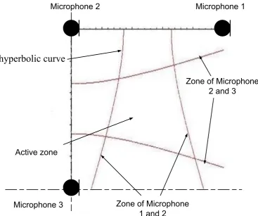
(5) 2.5.2.2 Detect a geometrical zone with three-microphone beamforming .............................. 34 2.5.2.3 Speech enhancement for automotive speech recognition in a car ............................. 36 2.5.3 SPEECH ENHANCEMENT FOR VOICE COMMUNICATION IN CAR ........................................ 39 2.5.3.1 An Adaptive filter in a car.......................................................................................... 39 2.5.3.2 An Wiener filter in a car ............................................................................................ 45 2.6 SUMMARY ........................................................................................................................ 47 3 PROBLEM DEFINITION AND RESEARCH ENVIRONMENTAL SET-UP .................. 49 3.1 PROBLEMS OF SPEECH ENHANCEMENT IN A CAR ............................................................... 49 3.2 APPROACHES ON SPEECH ENHANCEMENT IN A CAR .......................................................... 49 3.2.1 THREE-MICROPHONE VAD SWITCH AND NLMS FILTER ................................................ 50 3.2.2 WIENER FILTER IN 3 MICROPHONE ARRAY ..................................................................... 53 3.3 OVERVIEW OF SYSTEM BUILD-UP ..................................................................................... 53 3.4 RESEARCH ENVIRONMENTAL SET-UP................................................................................ 54 3.4.1 THREE-MICROPHONE DATA ACQUISITION IN CAR ........................................................... 54 3.4.2 SIGNAL CONDITIONING IN A CAR .................................................................................... 55 3.4.3 DIGITAL SIGNAL PROCESSING HARDWARE AND SOFTWARE ........................................... 58 3.5 SUMMARY ........................................................................................................................ 58 4 REAL-TIME ADAPTIVE NOISE CANCELLATION IN A CAR ..................................... 59 4.1 THREE-MICROPHONE BEAMFORMER IN A CAR .................................................................. 59 4.1.1 INTRODUCTION .............................................................................................................. 59 4.1.2 THREE MICROPHONE BEAMFORMING VOICE ACTIVITY DETECTION WITH ADAPTIVE NOISE CANCELLATION .................................................................................................... 59 4.1.3 THREE-MICROPHONE ADAPTIVE NOISE CANCELLATION ................................................. 60 4.1.4 A THREE-MICROPHONE VAD ......................................................................................... 61 4.1.5 SUMMARY AND DISCUSSION........................................................................................... 66 4.2 ADAPTIVE WIENER FILTER IN A CAR ................................................................................ 67 4.2.1 INTRODUCTION .............................................................................................................. 67 4.2.2 ADAPTIVE WIENER FILTER ............................................................................................. 67 4.2.3 MATRIX INVERSION METHOD ......................................................................................... 73 4.2.4 AUTOMATIC SPEECH RECOGNITION ............................................................................... 74 4.2.5 SUMMARY AND DISCUSSION........................................................................................... 76 5 EXPERIMENTS ................................................................................................................... 77 5.1 OVERVIEW ....................................................................................................................... 77 5.2 EXPERIMENTS – THREE MICROPHONE BEAMFORMING IN A CAR ....................................... 79 5.2.1 THREE-MICROPHONE VAD IN A CAR.............................................................................. 79 5.2.2 NLMS ADAPTIVE NOISE CANCELLATION IN 3-MICROPHONE BEAMFORMING IN A CAR ... 83 5.2.2.1 The 3-microphone noise canceller in a 2 speech environment .................................. 87 5.2.2.2 Definition of Noise canceller valid zone.................................................................... 89 5.2.2.3 A single noise environment: Driver’s voice and a stationary white noise ................. 91 5.2.2.4 A single noise environment: Driver’s voice and a second speech ............................. 93 5.2.3 AN ASR WITH 3-MICROPHONE VAD AND NLMS ANC ................................................ 95 5.2.4 COMPARISON OF NLMF AND NLMS ANC .................................................................... 96 II.

(6) 5.3 EXPERIMENTS – ADAPTIVE WIENER FILTER IN A CAR .................................................... 100 5.3.1 CASE STUDY ONE: COMPARISON OF ADAPTIVE WIENER FILTER UPDATE METHODS ...... 101 5.3.2 CASE STUDY TWO: ANALYSIS OF AVERAGE POWER IN THE SPECTROGRAMS ................. 104 5.3.3 CASE STUDY THREE: TEST IN RS-07 SPEECH RECOGNITION KIT .................................. 107 5.3.3.1 The inputs to the speech recognition successful rate without an adaptive Wiener filter . .................................................................................................................................. 107 5.3.3.2 The inputs to the speech recognition successful rate with an adaptive Wiener filter .... .................................................................................................................................. 110 5.3.3.3 Results of ASR successful rate with an AWF or without an AWF ......................... 112 5.3.4 CASE STUDY FOUR: TEST IN TEMPLATE MATCHING ASR IN LABVIEW ...................... 113 5.3.5 CASE STUDY FIVE: THE SIZE OF THE WIENER FILTER MATRIX ...................................... 117 5.3.6 CASE STUDY SIX: WIENER FILTER IN UNWANTED SPEECH FROM DIFFERENT LOCATIONS ... ..................................................................................................................................... 122 5.4 SUMMARY ...................................................................................................................... 127 6 CONCLUSIONS AND FUTURE WORK ......................................................................... 129 6.1 THE IMPROVEMENTS ON THE OTHER RESEARCHES.......................................................... 129 6.2 MAJOR FINDINGS AND CONTRIBUTIONS .......................................................................... 129 6.3 SUGGESTIONS FOR FUTURE WORK ................................................................................. 130 7 REFERENCE ...................................................................................................................... 132. III.

(7) Table of figures Figure 1-1 Three-microphone beamforming in car ................................................................ 1 Figure 1-2 Research objective ................................................................................................ 2 Figure 1-3 Hybrid noise cancellation approach ...................................................................... 3 Figure 1-4 Structure of this thesis........................................................................................... 6 Figure 2-1 Block diagram for a Real-Time Adaptive Acoustic noise cancellation for Automatic Speech Recognition in a Car Environment .............................................................. 7 Figure 2-2 A 2-microphone beamforming.............................................................................. 9 Figure 2-3 Delay-and-sum beamformer ............................................................................... 10 Figure 2-4 Griffiths-Jim beamformer ................................................................................... 13 Figure 2-5 RLS adaptive filter .............................................................................................. 15 Figure 2-6 LMS adaptive filter as noise canceller block diagram ........................................ 16 Figure 2-7 NLMS adaptive filter as noise canceller block diagram ..................................... 18 Figure 2-8 Chen and Moir's three-microphone system ........................................................ 35 Figure 2-9 Overview of adaptive beamformer history ......................................................... 47 Figure 3-1 non- stationary noise and interference ................................................................ 49 Figure 3-2 A hybrid system with acoustic beamforming VAD and an AWF ...................... 50 Figure 3-3 A desired zone is defined with 3 microphone..................................................... 52 Figure 3-4 Plan view of 3-microphone VAD valid zone in 3D............................................ 52 Figure 3-5 A modified adaptive Wiener filter with two microphone ................................... 53 Figure 3-6 Automobile environment layout ......................................................................... 54 Figure 3-7 Three microphones in a car ................................................................................. 55 Figure 3-8 Pre-amplifier ....................................................................................................... 56 Figure 3-9 Anti-alias filter .................................................................................................... 56 Figure 3-10 frequency respond ............................................................................................. 57 Figure 3-11 Pre-amplifier and anti-alias filter ...................................................................... 57 Figure 3-12 A block diagram of DSP hardware and software ............................................. 58 Figure 4-1 Overview of three-microphone VAD controlled three-microphone noise canceller ................................................................................................................................... 60 Figure 4-2 Three-microphone noise canceller block diagram .............................................. 61 Figure 4-3 Three-microphone VAD Block diagram ............................................................ 64 Figure 4-4 A defined active zone ......................................................................................... 64 Figure 4-5 A Wiener filter .................................................................................................... 68 IV.

(8) Figure 4-6 A Wiener filter with pre-computed W matrix .................................................... 69 Figure 4-7 W Matrix Calculation for single microphone case ............................................. 70 Figure 4-8 matrix updated during speech or noise period .................................................... 71 Figure 4-9 In-car test plan .................................................................................................... 72 Figure 4-10 A simple ASR block diagram ........................................................................... 75 Figure 5-1 Overview of experiments .................................................................................... 77 Figure 5-2 Eight testing points ............................................................................................. 79 Figure 5-3 An overview of testing unit in a car .................................................................... 80 Figure 5-4 Speech waveforms .............................................................................................. 81 Figure 5-5 NLMS adaptive filter as noise canceller block diagram ..................................... 84 Figure 5-6 Three-microphone noise canceller block diagram .............................................. 85 Figure 5-7 Definition of a noise canceller valid zone around microphone 1 ....................... 85 Figure 5-8 The 3-microphone noise canceller in a speech and unwanted speech environment ............................................................................................................................. 87 Figure 5-9 Refers to Figure 5-6, driver's voice enabled VAD (E = 1) and then disabled VAD (E = 0) ............................................................................................................................ 88 Figure 5-10 A test for the noise canceller valid zone ........................................................... 89 Figure 5-11 White noise source testing waveforms ............................................................. 90 Figure 5-12 Numbering the test points in a frequently moving noise sources environment (Driver’s voice and a second voice)......................................................................................... 91 Figure 5-13 Voice in the VAD valid zone activates the VAD, whilst a white noise source comes from test points 1, 2 and so on ...................................................................................... 92 Figure 5-14 Moving second voice (white noise) results....................................................... 92 Figure 5-15 Numbering the test points in a frequently moving noise sources environment (Driver’s voice and a second voice)......................................................................................... 93 Figure 5-16 E = 1 (as in Figure 6-6), other speech arrives via test points 1, 2 and 3 ........... 94 Figure 5-17 An ASR with 3-microphone VAD and NLMS ANC ....................................... 95 Figure 5-18 testing plan ........................................................................................................ 96 Figure 5-19 Testing of NLMF when A=0.1 ......................................................................... 97 Figure 5-20 Testing of NLMF when A=0.2 ......................................................................... 97 Figure 5-21 Testing of NLMF when A=0.3 ......................................................................... 97 Figure 5-22 Testing of NLMF when A=0.4 ......................................................................... 97 Figure 5-23 Testing of NLMF when A=0.5 ......................................................................... 98 Figure 5-24 Testing of NLMF when A=0.6 ......................................................................... 98 V.

(9) Figure 5-25 Testing of NLMF when A=0.7 ......................................................................... 98 Figure 5-26 Testing of NLMF when A=0.8 ......................................................................... 98 Figure 5-27 Testing of NLMF when A=0.9 ......................................................................... 99 Figure 5-28 Testing of NLMS .............................................................................................. 99 Figure 5-29 Experimental setup ......................................................................................... 101 Figure 5-30 The W matrix is updated during a noise period only or a speech activity period. (a) Wiener filter output (b) Waveform of Signal + noise from Microphone 2 (c) Waveform of noise from Microphone 1 ....................................................................................................... 102 Figure 5-31 W matrix is updated in real-time. (a) Wiener filter output (b) Waveform of signal + noise from Microphone (c) Waveform of noise from Microphone 1 ...................... 102 Figure 5-32 Spectrograms of the filtering process. The horizontal axis represents time (in seconds) and the vertical axis is frequency (in Hz) (a) clean speech “open the door” (b) Filtered speech (c) recording of Microphone1 (d) recording of Microphone2 (e) Intensity scale in dB .............................................................................................................................. 103 Figure 5-33 In-car test plan ................................................................................................ 104 Figure 5-34 Test results in a stationary car with engine and car radio on. ......................... 105 Figure 5-35 The spectrograms of the waveforms in Figure 6-34. The horizontal axis represents time (in second) and the vertical axis is frequency (in Hz). (a) Spectrogram at Microphone1. (b) Spectrogram at Microphone2. (c). Spectrogram of filtered signal. (d). Intensity scale in dB ............................................................................................................... 106 Figure 5-36 Test without an adaptive Wiener filter ........................................................... 107 Figure 5-37 records of “open the door” in low noise environment when the car radio and engine does not turn on .......................................................................................................... 108 Figure 5-38 Records of speech “open the door” in music environment by Microphone 1 108 Figure 5-39 Records of speech “open the door” in music environment by Microphone 2 109 Figure 5-40 Records of speech “open the door” in unwanted speech environment by Microphone 1 ......................................................................................................................... 109 Figure 5-41 Records of speech “open the door” in unwanted speech environment by Microphone 2 ......................................................................................................................... 110 Figure 5-42 Test with AWF................................................................................................ 110 Figure 5-43 Filtered speech “open the door” in music environment .................................. 111 Figure 5-44 Filtered speech “open the door” in unwanted speech environment ................ 111 Figure 5-45 The spectrograms of the waveforms of a female driver’s speech “right” and “left”. The horizontal axis represents time (in second) and the vertical axis is frequency (in VI.

(10) Hz). (a) Spectrogram at Microphone 1. (b) Spectrogram at Microphone 2. (c) Spectrogram of filtered signal. (d) Intensity scale in dB ................................................................................. 114 Figure 5-46 The spectrograms of the waveforms of a male driver’s speech “left” and “right”. The horizontal axis represents time (in second) and the vertical axis is frequency (in Hz). (a) Spectrogram at Microphone 1. (b) Spectrogram at Microphone 2. (c) Spectrogram of filtered signal. (d) Intensity scale in dB ................................................................................. 114 Figure 5-47 Design layout of hybrid noise canceller ......................................................... 117 Figure 5-48 Comparing of Frame size at spectrum of filtered speech in grey scale intensity ................................................................................................................................................ 119 Figure 5-49 The spectrograms of filtered speech whilst driver’s speech is incoming with simultaneous unwanted speech from radio loud-speakers or a passenger, in grey scale intensity .................................................................................................................................. 124 Figure 5-50 Summary of experiment.................................................................................. 127. VII.

(11) List of Tables Table 5-1 SNR improvement in different test zones ............................................................ 82 Table 5-2 Power of microphones inputs and noise canceller's output .................................. 90 Table 5-3 SNR results of white noise test ............................................................................ 90 Table 5-4 Result of AST successful rate in different source positions in 100 tests ............. 95 Table 5-5 SNR Analysis at average power ......................................................................... 106 Table 5-6 Results of test with AWF or without AWF ........................................................ 112 Table 5-7 Average power in dB result of cross-correlation between fingerprint "right" and 5 records of “right” or 5 records of “left” from a female driver ............................................... 115 Table 5-8 Average power in dB at result of cross-correlation between fingerprint "right" and 5 records of “right” or 5 records of “left” from a male driver ........................................ 115 Table 5-9 Average power in dB at result of cross-correlation between fingerprint "right" from a female driver and 5 records of “right” or 5 records of “left” from a male driver ...... 116 Table 5-10 Average power in dB at result of cross-correlation between fingerprint "right" from a male driver and 5 records of “right” or 5 records of “left” from a female driver ...... 116 Table 5-11 Average Power for different orders of W matrix ............................................. 120 Table 5-12 SNRs for different W matrix dimension obtained at an 11025 Hz sample rate ................................................................................................................................................ 120 Table 5-13 Average Signal Power Samples with reference to the seating positions referred to in Figure 5-49..................................................................................................................... 125 Table 5-14 Improved SNR with reference to Figure 5-49.................................................. 125. VIII.

(12) Abstract This research is mainly concerned with a robust method for improving the performance of a real-time speech enhancement and noise cancellation for Automatic Speech Recognition (ASR) in a real-time environment.. Therefore, the thesis titled, “Real-time adaptive. beamformer for Automatic speech Recognition in a car environment” presents an application technique of a beamforming method and Automatic Speech Recognition (ASR) method. In this thesis, a novel solution is presented to the question as below, namely: How can the driver’s voice control the car using ASR? The solution in this thesis is an ASR using a hybrid system with acoustic beamforming Voice Activity Detector (VAD) and an Adaptive Wiener Filter. The beamforming approach is based on a fundamental theory of normalized least-mean squares (NLMS) to improve Signal to Noise Ratio (SNR). The microphone has been implemented with a Voice Activity Detector (VAD) which uses time-delay estimation together with magnitude-squared coherence (MSC). An experiment clearly shows the ability of the composite system to reduce noise outside of a defined active zone. In real-time environments a speech recognition system in a car has to receive the driver’s voice only whilst suppressing background noise e.g. voice from radio. Therefore, this research presents a hybrid real-time adaptive filter which operates within a geometrical zone defined around the head of the desired speaker. Any sound outside of this zone is considered to be noise and suppressed. As this defined geometrical zone is small, it is assumed that only driver's speech is incoming from this zone. The technique uses three microphones to define a geometric based voice-activity detector (VAD) to cancel the unwanted speech coming from outside of the zone. In the case of a sole unwanted speech incoming from outside of a desired zone, this speech is muted at the output of the hybrid noise canceller. In case of an unwanted speech and a desired speech are incoming at the same time, the proposed VAD fails to identify the unwanted speech or desired speech. In such a situation an adaptive Wiener filter is switched on for noise reduction, where the SNR is improved by as much as 28dB. In order to identify the signal quality of the filtered signal from Wiener filter, a template matching speech recognition system that uses a Wiener filter is designed for testing. In this thesis, a commercial speech recognition system is also applied to test the proposed beamforming based noise cancellation and the adaptive Wiener filter.. IX.

(13) List of Abbreviations and Acronyms ANC. Adaptive Noise Canceller. ASR. Automatic Speech Recognition. AWF. Adaptive Wiener Filter. BSS. Blind Source Separation. DOA. Direction of Arrival. DFT. Discrete Fourier Transform. DS. Delay and Sum. DSP. Digital Signal Processing. EOD. Estimation of Direction. EOZ. Estimation of Zone. FFT. Fast Fourier Transform. FIR. Finite Impulse Response. GCC. Generalized Cross Correlation. GPS. Global Positioning System. GSC. Generalized Sidelobe Canceller. IDFT. Inverse Discrete Fourier Transform. IFFT. Inverse Fast Fourier Transform. IIR. Infinite Impulse Response. LabVIEW Laboratory Virtual Instrument Engineering Workbench LMS. Least Mean Square. MSC. Magnitude Squared Coherence. NLMS. Normalized Least Mean Squares. NLMF. Normalized Least Mean Forth. RLS. Recursive Least Square. SNR. Signal-to-Noise Ratio. TDOA. Time Difference of Arrival. VAD. Voice Activity Detector. X.

(14) Nomenclature μ. Step-size parameter for LMS. μn. A modified input dependent step size for NLMS. hn. Tap weight vector at time n of LMS or NLMS. ĥ n. Instantaneous estimate of the tap weight vector at time n. E[ ⋅ ]. Expectation operator. R xx ( k ). Discrete autocorrelation function of the input signal xn. R xd ( k ). Discrete cross-correlation function between xn and the desired response d n. Z. Z-transform operator. Φ xx ( z ). Z-transform auto power spectrum of the input signal xn. Φ xd ( z ). Z-transform cross power spectrum between the input signal xn and a desired response d n. R. E[ X n X nH ] , autocorrelation vector of tap input vector x n. P. E[ X n d n∗ ] , cross-correlation vector between the tap input vector x n and the desired response d n. xTn. Transposition input vector x n at time n. x nH. Hermitian transposition input vector x n at time n. δ (t ). Dirac delta function. ∧. S x1x1 (i ). ψg(f). General frequency weighting function. R (dg' x)' ( τ ). Generalized cross correlation function between d ' (t ) and x ' (t ). γˆdx ( f ). γ dx ( f ). Coherence estimate between x d (t ) and x x (t ) 2. Magnitude squared coherence function. λmax. The largest eigenvalue of the tap input auto correlation matrix R. β. Forgetting factor XI.

(15) G x1x2 ( f ). Cross-spectrum of x1 (t) and x2 (t) at frequency f. G x1x1 ( f ). Auto spectral density functions of x1 (t) at frequency f. G x2 x2 ( f ). Auto spectral density functions of x2 (t) at frequency f. γxx (f ). coherence between two zero-mean stationary random processes x1 (t). 1 2. and x2 (t), at frequency f d max. Maximum desired time-difference of arrival (TDOA) between two microphones. C min. Minimum desired MSC (with empirical meaning) to prevent reverberant speech from being detected as desired speech. XII.

(16) Acknowledgements First of all, I would like to express my sincere gratitude to my supervisor, Dr. Tom J. Moir for his invaluable guidance in his position as a top class world researcher in this field. From beginning to end, he has provided many opportunities for me to develop my research interests as well as his solid background in research expertise. Secondly, I would also like to thank to both Massey University and Unitec Institute of Technology for providing an excellent research and study environment, and financial support for the participation in international conferences.. XIII.

(17) Declaration I declare that the thesis is based on my own research work under the supervision of Dr. T. J. Moir during the Ph.D. study in School of Engineering and Advanced Technology, Massey University at Albany. The research work has produced a book chapter, journal papers, conference proceedings and presentations during the Ph.D. study. The content of this thesis therefore contains theory, procedure, application and experimental outputs from the research papers published during the research period as listed below. Book Chapter Qi, Z and Moir T (2008), An Adaptive Wiener Filter for Automatic Speech Recognition in a Car Environment with Non-Stationary Noise. In S. Mukhopadhyay & G. S. Gupta (Eds.), Smart Sensors and Sensing Technology: Springer-Verlag. Refereed journal paper Qi, Z., & Moir, T. J. (2006). Automotive 3-microphone Noise Canceller in a Frequently Moving Noise Source Environment. International journal of signal processing, 3 (4), 298304. Refereed conference proceedings Qi, Z., & Moir, T. (2008). Automotive speech control in a non-stationary noisy environment. Paper submitted at the 15th International Conference on Mechatronics and Machine Vision in Practice, Auckland, New Zealand. Qi. Z. & Moir. T. (2007). A Design of Automotive Voice Recognizer Using LabVIEW. Paper was accepted to The 14th Electronics New Zealand Conference (ENZCon). Wellington New Zealand. Qi, Z., & Moir, T. J. (2007). An Adaptive Wiener Filter for an Automotive Application with Non-Stationary Noise, Paper was accepted to 2nd International Conference on Sensing Technology 2007. Palmerston North, New Zealand.. XIV.

(18) Qi, Z., & Moir, T. J. (2005). An Automotive three-microphone Voice Activity Detector and noise canceller, 2005 International Conference on Intelligent Sensors, Sensor Networks and Information. Melbourne, 5 - 8 December, Melbourne. Qi, Z., & Moir, T. J. (2005). A geometrical active zone voice activity detector in car, 2nd IIMS Post-Graduate Conference. Auckland, 27 October. Non-refereed journal paper Qi, Z., & Moir, T. J. (2005). Automotive three-microphone Voice Activity Detector and noise-canceller. Research Letters in the Information and Mathematical Sciences, 7 (July 2005), 147-156, Institute of Information and Mathematical Sciences, Massey University, Auckland, New Zealand.. Candidate’s signature:. Candidate’s name: Ziming Qi. Date: 18-08-2008. XV.

(19)

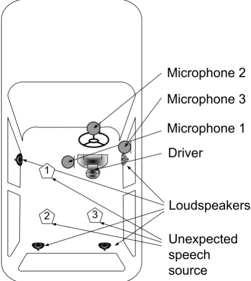
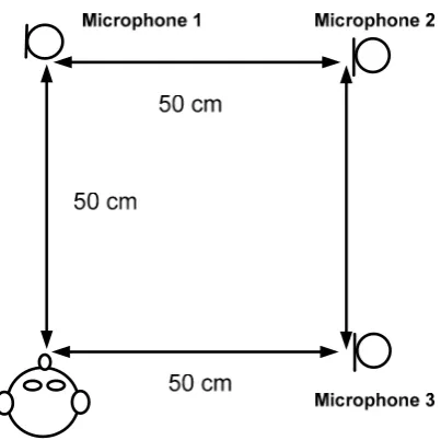
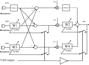
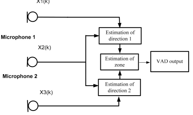
(20) Chapter 1 Introduction. 1 Introduction During the last several decades, a speech signal and array processing technology has been developed in various application areas. For a real-time application in real environments, using the driver’s voice to control some devices in the car is one of the most difficult challenges.. 1.1 Research objective The objective of this thesis is to simplify the use of microphones and reduce the real-time environment noise in order to control devices using Automatic Speech Recognition (ASR) successfully. As in Figure 1-1, a three-microphone beamforming is used to cancel the unwanted voice from passenger 1, 2 and 3 as well as from voice from the 4 loud-speakers. In the thesis, a hybrid Adaptive Noise Cancellation (ANC) is proposed, which uses a system with acoustic beamforming based Voice Activity Detector (VAD), Normalize least mean squares Adaptive filter and an Adaptive Wiener Filter as shown in Figure 1-2. Automatic Speech Recognition (ASR) is applied to test the quality of this hybrid ANC.. Microphone 2 Microphone 3 Microphone 1 Driver 1. 2. 3. Loudspeakers Unexpected speech source. Figure 1-1 Three-microphone beamforming in car. 1.

(21) Chapter 1 Introduction. Figure 1-2 Research objective. 2.

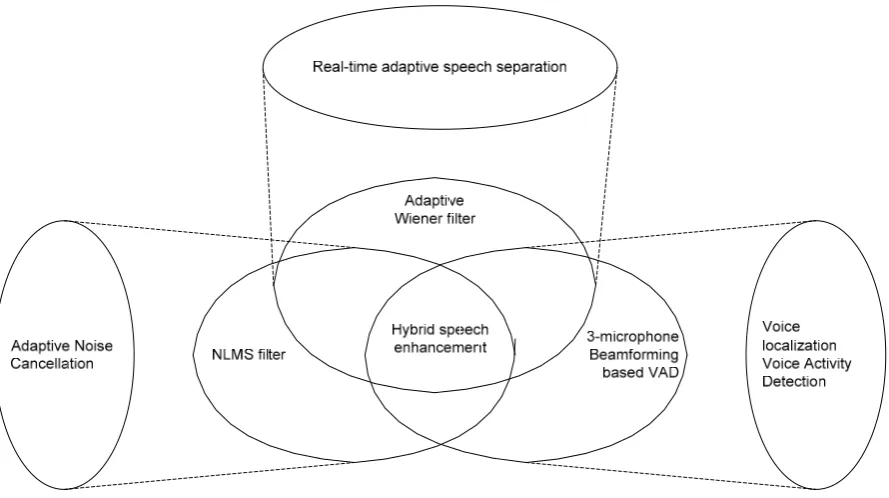
(22) Chapter 1 Introduction. 1.2 Speech enhancement approach In this thesis, the main approach is 3-microphone beamforming. A 3-microphone beamforming approved will be shown to be able to mute the input to ASR when voice or interference is incoming from outside of desired zone. When a desired command voice is incoming, a 3-microphone adaptive noise cancellation system can suppress the stationary noise in a car e.g. from a car engine. When non-stationary noise incoming e.g. from a car radio, an Adaptive Wiener filter is an addition to this main approach when the beamforming is “confused” by multi-source noise or interference. ASR is introduced in this thesis to switch the desired devices. There are three approaches in this thesis as in Figure 1-4: Adaptive noise cancellation, Real-time adaptive speech separation (using an adaptive Wiener filter) and Voice activity detection.. Figure 1-3 Hybrid noise cancellation approach 1.2.1 Voice activity detection approach. The Voice activity detection (VAD) approach is based on a fundamental theory of timedelay estimation with magnitude-squared coherence (MSC). An experiment will clearly show the ability of the composite system to reduce noise outside of a defined active zone. A 3microphone VAD approach is used in this thesis since it is relatively simple and not too much of a computational overload for real-time system. 3.

(23) Chapter 1 Introduction. 1.2.2 Adaptive noise cancellation approach in this thesis. Noise cancellation is based on a fundamental theory of normalized least-mean squares (NLMS) to improve Signal to Noise Ratio (SNR). The signal and noise inputs are shared with a Voice Activity Detector (VAD). A 3-microphone NLMS adaptive noise cancellation is used.. 1.2.3 Adaptive Wiener filter approach. Closely related to the NLMS approach is the technique used in this thesis which uses an adaptive Wiener filter. Whereas the NLMS approach uses weight estimation to minimize a mean-square error, this alternative approach constructs the Wiener filter from estimation of covariance matrices (for signal + noise and “noise-alone”). In real-time environments a speech recognition system in a car has to receive the driver’s voice only whilst suppressing background noise e.g. voice from radio. Therefore, this research presents a hybrid real-time adaptive filter which operates within a geometrical zone defined around the head of the desired speaker. Any sound outside of this zone is considered to be noise and suppressed. As this defined geometrical zone is small, it is assumed that only driver's speech is incoming from this zone. The technique uses three microphones to define a geometric based voice-activity detector (VAD) to cancel the unwanted speech coming from outside of the zone. However, when unwanted speech and desired speech are incoming at the same time, the VAD fails to identify the unwanted speech or desired speech. In such a situation, the adaptive Wiener filter is switched on for noise reduction. In the case of sole unwanted speech incoming from outside of a desired zone, this speech is muted at the output of the hybrid noise canceller. In the case of desired and unwanted speech incoming together, SNR is improved by as much as 28dB.. 4.

(24) Chapter 1 Introduction. 1.3 Contributions to knowledge In the thesis, the following original main contributions have been made: Firstly, 3-Microphone beamforming is applied in real-time to a car environment. The noisecancelling is only required when noise is present during desired speech since the VAD will mute any solo noise-source outside of the zone. The experiments in this thesis clearly show the ability of the composite system to reduce noise outside of a defined active zone. Secondly, a Wiener filter is used in this thesis, similar to the dual microphone method of Widrow et al except here Least-Mean Squares (LMS) is not used but instead is an update of the Wiener filter direct by estimation of the signal + noise and noise covariance matrices and by direct solution of the Wiener-Hopf equation. Thirdly, in this thesis, I suggest that it is not necessary for the enhanced signal to sound better to the human ear, but only needs to be good enough to provide a Boolean on or off command in all of these kinds of automated ‘smart-car’ technologies, (in contrast with some other similar technologies) although the filtered signals were clearly recognizable during informal listening tests and sounded vastly improved to the original. As an example, an ASR with Wiener filter has been designed to improve the recognition rate from 7 % up to 95%. Finally, a completed engineering model is presented in this thesis: a hybrid adaptive noise cancellation system, which employs 3-microphone voice activity detection with NLMS adaptive noise cancellation and an adaptive Wiener filter.. 1.4 Performance with favorable effects The beamforming and ASR approaches have provided an improved performance with some favorable effects to the three-microphone approach, such as the system allows voice controlled equipment available for a car in real-time environment. For example, drivers can control their car in noisy environments e.g. turn off the radio whilst the radio is on a news channel, or control devices whilst passengers are simultaneously speaking. Therefore, a fullvoice controlled car is available.. 5.

(25) Chapter 1 Introduction. 1.5 Structure of this thesis In chapter 2, a literature review will cover the relevant area of real-time adaptive acoustic noise cancellation for automatic speech recognition in a car environment. Chapter 3 will have the problem definition and research environmental set-up and Chapter 4 proposes the main solutions to such a problem. Chapter 5 has experiments to verify and confirm the solutions in the previous chapters. Finally, a design method of hybrid adaptive noise cancellation is discussed in Chapter 6 Conclusions and Future Work. The structure of this thesis is shown in Figure 1-4.. Chapter 1 Introduction. Chapter 2 Literature review. Chapter 3 Problem definition and research environmental set-up. Chapter 4 Noise cancellation in a car. Chapter 5 Experiments. Chapter 6 Conclusions and Future Work. Figure 1-4 Structure of this thesis. 6.

(26) Chapter 2 Literature review. 2 Literature review 2.1 Introduction In this chapter, the literature review explores the technical background in an area of microphones, signal conditioning and adaptive digital signal processing to propose a realtime adaptive acoustic noise cancellation for automatic speech recognition in a car environment as showed in Figure 2-1.. Figure 2-1 Block diagram for a Real-Time Adaptive Acoustic noise cancellation for Automatic Speech Recognition in a Car Environment In a car environment, a controlled object could be any device e.g. a window, a radio or a GPS. However, the purpose of this thesis is not to discuss such a control object. The focus is the method of a real-time adaptive noise cancellation for automatic speech recognition in a car environment. In Figure 2-1, microphone and signal conditioning are very important hardware support to this research. DSP hardware is the main body of digital signal processing. More importantly, this thesis will discover the best solution to enhance speech in a car. Therefore, the literature review will include acoustic beamforming, voice activity detection, the cocktail party effect and solution, speech enhancement in a car noise environment and also digital signal processing hardware and software.. 7.

(27) Chapter 2 Literature review. 2.2 Acoustic beamforming 2.2.1 Overview. Acoustic beamforming consists of signal processing using arrays of microphones to control the directionality and sensitivity of sound. Such a beamformer can be either a receive beamformer or transmit beamformer. In a receive beamformer, beamforming can increase the receiver sensitivity in the desired direction and decrease the sensitivity in the unwanted direction. As an example, the human brain uses a form of signal processing on its ears and determines sound localization. In transmit beamformer, beamforming can increase the power in a given direction(Beamforming, 2008). As early as 1969, Capon (Capon, 1969) proposed a minimum variance distortionless response (MVDR) beamformer which these results were given to seismic data obtained from the large aperture seismic array located in eastern Montana. Acoustic beamforming techniques can be divided into two categories: Acoustic conventional beamformer and Acoustic adaptive beamformer. An acoustic conventional beamformer is a fixed beamformer. An acoustic adaptive beamformer is an adaptive array of microphones. An acoustic conventional beamformer uses a fixed set of weightings and time-delays to combine the signals from the microphones in the array whilst an acoustic adaptive beamformer is able to adapt automatically its response to different weightings or time-delays. In the acoustic adaptive beamformer, a criterion is built up to allow the adaptation to minimize the noise output. In wide band systems, acoustic adaptive beamformer is very often to be considered to process in the frequency domain(Beamforming, 2008).. 8.

(28) Chapter 2 Literature review. 2.2.2 Conventional “delay and sum” acoustic beamformer. A 2-microphone acoustic beamforming is shown in Figure 2-2. Figure 2-2(a) is shown as both of microphones receive incoming sound at the same time. It means sound from an acoustic source reaches the two microphones from an equal distance. Figure 2-2(b) is shown that the incoming wave front reach the right microphone first and then the left microphone. Since microphones across the array receive signals with differential time delays, the microphones outputs no longer add coherently and cause the output of sum drops. Figure 2-2(c) is shown that there is a delay between the right microphone and an input of signal processer. While this delay equals to differential time delay of arrival of right microphone and left microphone, beamforming output is assumed as same as at Figure 22(a). Therefore a time delay at one of the two signal channels, output will enhance the sound source incoming from a desired direction.. (a). (b). (c). Incoming signal. Microphone array Delay Signal processing Signal output Figure 2-2 A 2-microphone beamforming If there are more than two microphones, e.g. n microphones in Figure 2-3, time delays with fixed values are set up at each signal processing channel. The received signals from the microphones are then delayed by different values and finally is summed to emit as Y(k). This beamformer is normally called a delay-and-sum beamformer. 9.

(29) Chapter 2 Literature review In delay–and-sum beamformer, while the incoming signal is x(k ) and k is 1, 2 … n, x ( k ) = [ x1 ( k ),..., x M ( k )] T. (2.1). The output of the beamformer is: y (k ) = w H x(k ). (2.2). H. The w denotes the complex conjugate transpose of the weight vector w, w = [ w1 ,..., w M ]T. X 1 (k ). X 2 (k ). (2.3). X 3 (k ). X n (k ). Y (k ). Figure 2-3 Delay-and-sum beamformer An n-microphone receiving beamformer takes advantage of interference to change the directionality of the array. On the other hand, a transmit beamformer can control the phase and relative amplitude of the signal at each transmitter to create a pattern of constructive and destructive interference in the wavefront. As an example, Hodgkiss (Hodgkiss, 1980) designed a programmable time-delay-and-sum digital beamformer, which permits the incorporation of slow changes in element positions and/or beam steering direction while the beamformer carries out the real-time formation of 1300 beams from 32 input sensors. This thesis only considers receive beamformers.. 10.

(30) Chapter 2 Literature review. 2.2.3 Far-field and Near-field acoustic wavefronts. Conventional analysis and synthesis techniques for microphone arrays are based on the simplifying assumption that all acoustic sources are located far from the array. In this case wavefront curvature can be neglected and all waves impinging upon the array are assumed to be planar (Ryan & Goubran, 1997). However, when the microphone array receives the sound which is near by, the sound wavefront does not appear as planar. Mailloux suggested (Mailloux, 1994) the far-field assumptions are no longer valid when 2 d dod fs r< (2.4) c with r the distance of the signal source to the centre of the microphone array,. d dod = d N −1 − d 0 the total length of the microphone array, f s the sampling frequency and c the speed of sound. In Figure 2-2 and 2-3, the incoming signal wavefronts can be planar in case of far-field assumptions. However, in this thesis, the total length of microphone array in a car is 1 m; the sampling frequency is 11025 Hz. The r from equation 2.4 will be 32 m. Since the distance of signal source (a driver in a car) to the centre of microphone array is less than 0.5 m, we will consider near-field acoustic wavefronts in any cases in this thesis.. 11.

(31) Chapter 2 Literature review. 2.2.4 Adaptive Acoustic Beamforming. An adaptive beamformer is a signal processing system which applies an algorithm to adjust an array in real-time. A typical application is an array of radar antennas which is to transmit or receive signals in different directions without mechanical steering. An adaptive acoustic beamformer has the ability to adjust its performance to suit differences in its environment e.g. reducing sensitivity to the directions of arrival where unwanted noise or interference is incoming. Adaptive Beamforming often employs Least Mean Squares (LMS) Algorithm to adjust an array in real-time to enhance the desired signal and cancel the noise or interference. As early as 1970s, Frost (Frost, 1972) applied a constrained least mean-squares algorithm which is capable of adjusting an array of sensors in real time to respond to a signal coming from a desired direction while unwanted noises coming from other directions. Analysis and simulations confirm that this algorithm is able to iteratively adapt variable weights on the taps of the sensor array to minimize noise power in the array output. A set of linear equality constraints on the weights keeps a chosen frequency characteristic for the array in the desired direction. Ferrara and Widrow (Ferrara & Widrow, 1981) also applied an adaptive algorithm to enhance a signal against noise. It used two or more input channels containing correlated signal components but uncorrelated noise components. The output is a best least squares estimate of the underlying signal in a chosen input channel. They stated that the more input channels available containing correlated signal components, the better will be the system performance. Excellent performance is obtained when the sum of the filter input signal-tonoise ratios (SNR), is large compared to unity at all frequencies of interest. In this case the output noise is small, the output signal distortion is small and the output SNR is approximately equal to the sum of the filter input SNR. However, this beamformer can improve signal-to-noise ratio (SNR) from a desired direction but cannot cut off the sound or noise which came from outside of this direction. The signal-to-noise ratio (SNR) of the total signal is greater than (or at worst, equal to) that of any individual microphone’s signal. This system makes the array pattern more sensitive to sources from a particular desired direction (Sullivan, 1996). In fact, most applications use acoustic beamforming to enhance desired direction sound source and also use other algorithms to improve signal-to-noise ratio (SNR). The most popular one is a digital filter. 12.

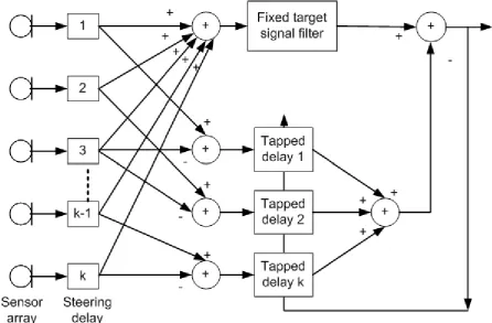
(32) Chapter 2 Literature review Griffiths and Jim (1982) described an adaptive beamformer as Figure 2-4.. Figure 2-4 Griffiths-Jim beamformer As in Figure 2-4, this beamformer consists of the summing process from the delay-and-sum beamformer, to provide an enhanced desired signal component, and an adaptive multichannel section which uses the differences between the time-aligned input signals to provide a representation of the undesired signal components. This simple beamformer shown above consists of a main antenna and one or more auxiliary antennas. The main antenna on the top is highly directional and is pointed in the desired signal direction. It is assumed that the main antenna receives both the desired signal and the interfering signals through its sidelobe (this beamformer is also known as sidelobe noise canceller). The auxiliary antenna primarily receives the noise or interfering signals since it has very low gain in the direction of the desired signal. The auxiliary array weights are chosen such that they cancel the interfering signals that are present in the sidelobe of the main array response. Later Krolik et al. (Krolik, Eizenman, & Pasupathy, 1986) used adaptive beamforming with generalized correlation (GC) to demonstrate a means of time delay estimate (TDE) bias reduction in interference dominated environments. They gave analysis of GC TDE bias with both. minimum. variance. distortionless. response. and. conventional. delay-and-sum 13.

(33) Chapter 2 Literature review beamforming. At high interference-to-noise ratios, theoretical and simulation results indicated that the adaptive structure can facilitate improved delay estimation performance compared to conventional methods. In 2004, Dmochowski and Goubran (J. Dmochowski & Goubran, 2004) presented a noise cancellation structure with a fixed beamformer front end. Simulation results showed a noise reduction of 21 dB with a speech source-noise source separation of 1 meter. The experimental results showed a complex noise reduction pattern with a maximum noise reduction of 17 dB. Dmochowski and Goubran (J. Dmochowski & Goubran, 2005) also examined in 2005 a microphone array based, combined beamformer noise canceller structures. The performance of the structures was evaluated using computer simulation as well as experimental measurements. The inter-operation of the beamformer and noise canceller was measured under the SNR. An experimental procedure for evaluating output SNR was presented in their research: the desired signal was captured from a set location in the recording environment. The noise signal was measured from a second location. Results revealed an SNR improvement of up to 17 dB. More recently Dmochowski and Goubran (J. P. Dmochowski & Goubran, 2007) informed that the enhancement of noise-corrupted speech acquired by microphones is indispensable to the functioning of a wide variety of digital signal processing algorithms. As many existing products are equipped with steerable, stand-alone fixed beamformers which provide moderate levels of directivity, these applications have long employed the classical adaptive noise canceller configuration with a reference sensor near the noise source to cancel unwanted noise. In their research, the cascading of stand-alone beamformers with back-end adaptive noise cancellers was presented. A decoupled model for signal enhancement using front-end beamformers and cascaded noise cancellers was also presented. The inter-operation of the beamforming and noise cancelling units was studied by defining the signal-to-interference ratio (SIR) gain, directivity index, and white noise gain offered by the beamforming and noise cancelling components. An experimental result shows the SIR improvement as much as to 27 dB.. 14.

(34) Chapter 2 Literature review. 2.2.5 Adaptive algorithm for beamforming 2.2.5.1 Recursive Least Square algorithm. The RLS algorithm uses an adaptive method to determine the coefficients of an adaptive filter. The method utilizes information from all the previous input data to estimate the inverse of the autocorrelation matrix of the input vector (S. Haykin, 1996). It has been derived independently by several investigators, but the original reference on the RLS algorithm is appeared to be Plackett in 1950 (Plackett, 1950). RLS adaptive filter block diagram is shown as Figure 2-5. Desired Signal d ( k ) + Input Signal x(k ). Input Signal x(k ). Output Signal y (k ). ErrorSignal e(k ). Figure 2-5 RLS adaptive filter. The recursive method of least squares is to minimize the residual sum of squares of the error signal e(k ) . To adjust of influence of input samples from the far past, the weighting factor is used in the cost function J (k ) . k. J (k ) = ∑ β k −i e 2 (i ). (2.5). i =1. where β is the exponentially weighted forgetting factor. It is selected between 0 < β < 1 . The resulting equation for the optimum filter coefficients at time k is, h(k ) = R −1 (k )Ρ(k ). (2.6). k. where. R (k ) = ∑ β k −i x(i )x H (i ) i =1. k. and. Ρ(k ) = ∑ β k −i d (i )x H (i ) i =1. .. 15.

(35) Chapter 2 Literature review Both R (k ) and Ρ(k ) can be computed recursively: R (k ) = β R (k − 1) + (1 − β )x(k )x H (k ). (2.7). Ρ(k ) = β Ρ(k − 1) + (1 − β )d (k )x(k ) (2.8) −1 To find the coefficient vector h(k ) , we need the inverse matrix R ( k ) . Using a matrix inversion lemma (S. Haykin, 1996), a recursive update equation for R −1 ( k ) is found as R −1 (k ) = β −1 R −1 ((k − 1) + β −1 μ ' (k )x(k ). μ ' (k ) = where. (2.9). β R (k − 1)x(k ) −1. −1 1. 1 + β −1 x H (k )R −1 (k − 1)x(k ). Therefore, we find the weights update equation as h(k ) = h(k − 1) + μ ' (k )(d (k ) − x(k )h(k − 1)). (2.10). For the computational complexity, RLS requires 5 N + 2 N + 2 multiplications (Lim, 1994). 2. 2.2.5.2 Least Mean Square algorithm. Least mean squares (LMS) algorithms are used in adaptive filters to find the filter coefficients that relate to producing the least mean squares of the error signal (difference between the desired and the actual signal). It is a stochastic gradient descent method in that the filter is only adapted based on the error at the current time. It was invented in 1960 by Bernard Widrow and Ted Hoff (Least mean squares filter, 2008). A LMS filter block diagram is shown as Figure 2-6. Desired Signal d (k ) + Input Signal x(k ). Input Signal x(k ). Output Signal y (k ). ErrorSignal e(k ). Figure 2-6 LMS adaptive filter as noise canceller block diagram As in Figure 2-6, LMS adaptive filter equations is shown as below: (Bellanger, 2001; Diniz, 2002; Ifeachor, 1993; Lyons, 2004; Rorabaugh, 1999). 16.

(36) Chapter 2 Literature review n −1. y ( n ) = ∑ wk ( n ) • x ( n − k ). (2.11). e(n) = d (n) − y(n). (2.12) (2.13). k =0. w k ( n + 1) = w k ( n ) + 2 μe( n ) x ( n − k ). Where k = 1, 2 …, N - 1. To define the self learning process the filter uses, adaptive algorithm is selected to reduce the error between the output signal y(k) and the desired signal d(k). When the LMS performance criteria for e(k) has achieved its minimum value through the iterations of the adapting algorithm, the adaptive filter is finished and its coefficients have converged to a solution. Now the output from the adaptive filter matches closely the desired signal d(k). If the input data characteristics are changed, sometimes called the filter environment, the filter adapts to the new environment by generating a new set of coefficients for the new data. Notice that when e(k) goes to zero and remains there you achieve perfect adaptation; the ideal result but not likely in the real world(Lyons, 2004). 2.2.5.3 Normalized least mean square algorithm. In the LMS algorithm the selection of step size ( μ ) may affect its stability and the convergence rate. When μ is too large, it has faster convergence but less stability. On the other hand, if μ is smaller, it has slower convergence but greater stability. Therefore a LMS has difficulties in a real-time processing in a real environment since a speech has a wide dynamic range and may give rise to stability in quiet utterances and conversely instability when the utterances are louder or when non stationary noise is added. Haykin (Haykin, 1996) suggested that the LMS algorithm can be convergent or stable in the mean, if and only if 0<μ <. 2. λ max. . Using the analysis that the maximum value of μ depends on the largest. eigenvalue λ max of the input autocorrelation R, which can be approximated to tr (R ) and then in the same way to x n. 2. 2. (i.e., λ max ≈ tr (R ) ≈ x n ), it can be induced that the maximum. value of μ depends on the input power signal. Accordingly, the step size for the stable adaptation has to be constrained according to 0 < μ <. 2. λ max. ≈. 2 2 ≈ tr ( R ) xn. 2. , where, λ max is. the largest eigenvalue of the tap input auto correlation matrix R , tr (R ) is trace of R , which P. is the sum of the elements on its diagonal ( ∑ λi ), and x n is the input power. 2. i =1. 17.

(37) Chapter 2 Literature review Based on the above, normalize least mean squares (NLMS) algorithm is used in adaptive filtering algorithms due to its simplicity for real-time applications. (Simon. Haykin, 2002) A NLMS filter block diagram is shown as Figure 2-7. To define the self learning process the filter uses an adaptive algorithm to reduce the NLMS between the output signal y(k) and the desired signal d(k). For stationary signals, when the NLMS performance criteria for the NLMS have achieved its minimum value through the iterations of the adapting algorithm, the adaptive filter is finished and its coefficients have converged to a constant solution. Then the output from the adaptive filter matches closely the desired signal d(k). If the input data characteristics are changed, the filter adapts to the new environment by generating a new set of coefficients for the new data. The e(k) goes to zero and remains there.. Figure 2-7 NLMS adaptive filter as noise canceller block diagram The NLMS adaptive filter weights are updated accordingly (Barrault, Costa, Bermudez, & Lenzi, 2005) W k +1 = W k + 2μ n e k X k. (2.14). Wk = [ w1,k w2,k ... wN ,k ]T. (2.15). Where the weight vector are the coefficients of the adaptive filter at time k,. X k = [ x k x k −1 ... x k − N +1 ]T are the N samples of the input data in filter memory at time k,. (2.16). e k = d k − W kT X k. (2.17). μn =. (2.18). μ~. δ + xn. 2. 18.

(38) Chapter 2 Literature review Where 0 < μ~ < 1 ,. μ n is a modified input dependent step size and δ is an infinitesimal. positive value added to prevent the possibility of zero division in the event of a very small input value. where δ = 0.0001 Xk. 2. and. Xk. is. Euclidean. norm. of. Xk. and. is. given. by. = x k2 + x k2−1 + ... x k2− N +1 .. When Microphone 1 is defined as the primary input and Microphone 2 as the reference input, as in Figure 1, experiments (Rulph, 2002) show that voice close to the primary input is enhanced while voice close to the reference input is reduced. 2.2.5.4 Normalized Least Mean Forth algorithm. Walach and Widrow (Walach & Widrow, 1984) presented a steepest descent algorithms for adaptive filtering and have been devised which allow error minimization in the mean fourth. Ideally, during adaptation, the weights undergo exponential relaxation toward their optimal solutions. Time constants have been derived, and surprisingly they turn out to be proportional to the time constants that would have been obtained if the steepest descent least mean square (LMS) algorithm of Widrow and Hoff had been used. The gradient algorithms are insignificantly more complicated to program and to compute than the LMS algorithm. Conditions have been derived for weight-vector convergence of the mean and of the variance for the new gradient algorithms. The behavior of the least mean fourth (LMF) algorithm is of special interest. In comparing this algorithm to the LMS algorithm, when both are set to have exactly the same time constants for the weight relaxation process, the LMF algorithm, under some circumstances, will have a substantially lower weight noise than the LMS algorithm. It is possible, therefore, that a minimum mean fourth error algorithm can do a better job of least squares estimation than a mean square error algorithm. This intriguing concept has implications for all forms of adaptive algorithms, whether they are based on steepest descent or otherwise. Recently Zerguine (Zerguine, 2000) presented a NLMF algorithm. It sounds that NLMF had shown to have potentially faster convergence than NLMS. Unlike the LMF algorithm, the convergence behaviour of the NLMF algorithm is independent of the input data correlation statistics. Sufficient conditions for the NLMF algorithm convergence in the mean were obtained and the analysis of the steady-state performance was carried out using the feedback approach. Simulation results confirmed the performance of the NLMF algorithm.. 19.

(39) Chapter 2 Literature review However, Zerguine (Zerguine, 2000) stated that NLMF algorithm results in the fastest average convergence for a gradient step: this was of course at the expense of higher misadjustment values. Moinuddin et al (Moinuddin, Zerguine, & Sheikh, 2005) had tracking analysis of the normalized least mean fourth (NLMF) algorithm, which is carried out in the presence of two sources of non-stationeries (carrier frequency offset between transmitter and receiver, and random variations in the environment). The concept of energy conservation was used to carry out the analysis. Simulation results agreed very closely with theory. The results showed that, unlike in the stationary case, the steady-state excess mean-square error (MSE) was not a monotonically increasing function of the step size. Moreover, the ability of the adaptive algorithm to track the variations in the environment is shown to degrade with increasing frequency offset. In summary, LMF algorithm is known for its fast convergence and lower steady state error, especially under sub-Gaussian noise conditions. Meanwhile, the recent work on the normalised versions of LMF algorithm has further enhanced its stability and performance in both Gaussian and sub-Gaussian noise. For example, the XE-NLMF algorithm is normalised by the mixed signal power and error power, and weighted by a fixed mixed-power parameter. Unfortunately, this algorithm depends on the selection of this mixing parameter. Chen et al (2003) introduced a time-varying mixed-power parameter technique to optimise its selection. An enhancement in performance is obtained through the use of this procedure in both the convergence rate and steady-state error. (Chan, Zerguine, & Cowan, 2003) Nascimento and Bermudez in 2005 described that the least-mean fourth and the least-mean mixed norm algorithms are not mean-square stable when the input is Gaussian-distributed. (Nascimento & Bermudez, 2005) Zerguine (Zerguine, 2000) described the LMF adaptive filter weights are updated accordingly. Wk +1 = Wk + 2 μek3 X k. (2.19). Wk = [ w1,k w2,k ... wN ,k ]T. (2.20). Where the weight vector. are the coefficients of the adaptive filter at time k,. X k = [ x k x k −1 ... x k − N +1 ]T. (2.21). are the N samples of the input data in filter memory at time k,. ek (n) = d k (n) − WkT X k. (2.22) 20.

(40) Chapter 2 Literature review is the error between the adaptive filter output and the desired signal d k and μ is a user specified convergence parameter which if chosen to be too small will lead to slow convergence. If chosen to be too large the LMF algorithm will become unstable and the weights will diverge. To overcome this problem in a non-stationary environment we use the NLMF algorithm. The NLMF algorithm is given by (Zerguine, 2000) Wk +1 = Wk + 2 μ~ek3. Xk Xk. 2. +δ. (2.23). ~ < 1 , δ = 0.0001 and X is Euclidean norm of X and is given by Where 0 < μ k k 2. (2.24) X k = x k2 + x k2−1 + ... x k2− N +1 In this thesis, an experiment in Chapter 5 computes NLMF and NLMS performances for noise cancellation.. 21.

(41) Chapter 2 Literature review. 2.2.6 Robust acoustic adaptive beamforming Although in the preceding discussion on the adaptive acoustic beamformers are considered as a good resolution to background noise and interference, the adaptive acoustic beamformers are much more sensitive to errors compared with conventional acoustic beamformers, such as the array steering vector errors caused by imprecise sensor calibrations (J. Li & Stoica, 2005). Therefore, over the past decades, much effort has been devoted to build robust adaptive beamformers. Adaptive beamforming algorithms are sensitive to small errors in array characteristics. In their new book in 2007, Li et al. (J. Li & Stoica, 2005) presented their research developments on robust adaptive beamforming. They had concluded that most of the early methods of making the adaptive beamformers more robust to array steering vector errors are rather ad hoc in that the choice of their parameters is not directly related to the uncertainty of the steering vector, until recently an uncertainty set of the array steering vector had been proposed. They had suggested four areas of current concerns on Robust Adaptive Beamforming: Array steering vector uncertainty, the finite sample size effect, the signal waveform estimation, constant modulus algorithms and robust wideband beamforming.. 22.

(42) Chapter 2 Literature review. 2.3 Voice Activity Detection Voice activity detection (VAD) is an algorithm used in detecting the presence of human speech from silence, music, noise or other non-speech signals. In this thesis, VAD is also used to separate the desired speech from unwanted speech (Qi & Moir, 2005). The typical applications of VAD are in speech coding and speech recognition (Moir, 2008).. 2.3.1 Time delay estimation As one of important VAD methods, in this thesis, estimation theory is applied. The goal of VAD is to gather the values of disturbance parameters e.g. noise variance, signal parameters e.g. amplitude or propagation direction, or signal waveforms. Estimation theory assumes that the observations contain an information-bearing quantity, thereby tacitly assuming that detection-based pre-processing has been performed. Conversely, detection theory often requires estimation of unknown parameters: Signal presence is assumed, parameter estimates are incorporated into the detection statistic, and consistency of observations and assumptions tested. Consequently, detection and estimation theory form a symbiotic relationship, each requiring the other to yield high-quality signal processing algorithms. (Johnson, 2003) At best, estimation theory is less structured than detection theory. Detection is science, estimation art. Inventiveness coupled with an understanding of the problem e.g. what types of errors are critically important, are key elements to deciding which estimation procedure "fits" a given problem well (Johnson, 2003). In speech recognition, word boundary detection is a main method. In spoken language, there are no gaps between words; where to place the word boundary often depends on what choice makes the most sense grammatically and given the context. In written form, languages e.g. Chinese do not have word boundaries either. Therefore, an estimation theory is suitable for the purpose of word boundary detection. Time delay estimates are used to locate the position of voice source. The main method is time domain cross correlation. The cross correlation between two zero-mean stationary random processes x1 (t) and x2 (t) is defined as (Myers, Erim, & Lowery, 2004):. R x1x2 (τ ) = E[ x1 (t ) x 2 (t + τ )]. (2.25). where E [·] is the estimation operator. Assuming periodicity, for single time-limited realizations of each random process, this is determined using the integral:. R x1x2 (τ ) =. ∞. ∫x. * 1. (t ) x 2 (t + τ )dt. (2.26). −∞. where * denotes complex conjugation and τ is the time lag between the signals. The Fourier transform of the cross correlation function, defines the cross-spectrum, G x1x2 ( f ) . Cross 23.

(43) Chapter 2 Literature review correlation functions are unbounded measures and are typically normalized by the values of the autocorrelations at zero lag to bound the estimate between -1 and 1. The autocorrelation functions are the time domain equivalent of the auto power spectra and their value at zero lag represents the total energy in the signal. The normalized and bounded measure is known as the cross correlation coefficient, ρ x1 x2 (τ ) , which provides a measure of the linear association between the two signals at a given time lag and is given by: R x1x2 (τ ). ρ x x (τ ) =. (2.27). R x1x1 (0) R x2 x2 (0). 1 2. represents the time series as a binary pulse train with ones corresponding to the firing times of the signals. A moving average window is then used to smooth these binary signals, which is analogous to filtering the time-series with a low-pass filter (Myers et al., 2004). 2.3.2 Magnitude squared coherence. Magnitude Squared Coherence (MSC) is a frequency domain method which can be applied to voice activity detection. Carter et al. (1973) (Carter, Knapp, & Nuttall, 1973) describe a method for estimating the magnitude-squared coherence function for two zero-mean widesense-stationary random processes is presented. The estimation technique utilizes the weighted overlapped segmentation fast Fourier transform app roach. Analytical and empirical results for statistics of the estimator are presented. The analytical expressions are limited to the non-overlapped case; empirical results show a decrease in bias and variance of the estimator with increasing overlap and suggest a 50-percent overlap as being highly desirable when cosine (Hanning) weighting is used. The coherence between two zero-mean stationary random processes x1 (t) and x2 (t), at frequency f, is defined as:. γxx (f) = 1 2. G x1 x2 ( f ) [G x1 x1 ( f )G x2 x2 ( f )]. 1. (2.28) 2. where G x1x2 ( f ) is the cross spectral density and G x1x1 ( f ) and G x2 x2 ( f ) are the auto spectral density functions of x1 (t) and x2 (t) respectively. The coherence function is a complex quantity and its squared magnitude provides a bounded measure of linear association between the two series, taking on a value of 1 for a perfect linear relationship and a value of 0 to indicate that the series are uncorrelated. In practice, it is necessary to estimate the magnitude squared coherence, C x1x2 ( f ) =| γ x1 x2 ( f ) | 2 , by windowing the time series to obtain multiple sections as follows:. 24.

No results found